TOWARDS THE OPTIMAL OPERATION OF AN ORGANIC RANKINE
CYCLE UNIT BY MEANS OF MODEL PREDICTIVE CONTROL
Andres Hernandez1,2*, Adriano Desideri2, Clara Ionescu1, Sylvain Quoilin2, Vincent Lemort2, Robin De Keyser1
1Ghent University, Department of Electrical energy, Systems and Automation, Ghent, Belgium
[email protected], [email protected], [email protected]
2University of Liège, Aerospace and Mechanical engineering department, Liège, Belgium
[email protected], [email protected], [email protected] * Corresponding Author
ABSTRACT
In this paper the optimal operation of an Organic Rankine Cycle (ORC) unit is investigated both in terms of energy production and safety conditions. Simulations on a validated dynamic model of a real re-generative ORC unit, are used to illustrate the existence of an optimal evaporating temperature which maximizes energy production for some given heat source conditions. This idea is further extended using a perturbation based Extremum Seeking (ES) algorithm to find online the optimal evaporating tempera-ture. Regarding safety conditions we propose the use of the Extended Prediction Self-Adaptive Control (EPSAC) approach to constrained Model Predictive Control (MPC). Since it uses input/output models for prediction, it avoids the need of state estimators, making of it a suitable tool for industrial applica-tions. The performance of the proposed control strategy is compared to PID-like schemes. Results show that EPSAC-MPC is a more effective control strategy as it allows a safer and more efficient operation of the ORC unit, as it can handle constraints in a natural way, operating close to the boundary conditions where power generation is maximized.
1. INTRODUCTION
In recent years several studies have underlined the potential of low-grade heat recovery to reduce the amount of worldwide industrial energy consumption (IEA, 2010). The highly fluctuating nature of the heat source makes waste heat recovery (WHR) applications a challenging task. Organic Rankine Cycle (ORC) systems represent the most promising technology for WHR, where the main objectives to op-timally operate the system are twofold: 1) keep the cycle in a safe condition and 2) maximize the net output power.
Safe operation of the ORC unit is important as it allows a longer life expectancy in all components. In this regard, an accurate regulation of the superheating represents an important task for the controller. The regulator has to guarantee a minimum value of superheating in order to maximize the efficiency, and to avoid the formation of liquid droplets at expander inlet that can damage the expansion machine (Wei et al., 2007). On the other hand, in order to maximize the output power, the evaporating temperature represents the most relevant controlled variable (Quoilin et al., 2011; Hernandez et al., 2015).
In this contribution we propose a two-layer control structure to guarantee the optimal operation of an ORC unit for waste heat recovery applications: an Extremum Seeking (ES) algorithm to find on-line the optimal evaporating temperature, which is later given as reference to a constrained Model Predictive Controller (MPC).
Extremum Seeking is a well developed research area which addresses the problem of objective value optimization when the objective function, its gradient and optimum value are unknown (Ariyur and
Krstic, 2003). In this study we make use of a perturbation based ES to find the evaporating temperature that maximizes the output power for the case of heat source variations. The performance of the ES algorithm is compared to the correlation obtained directly from the dynamic nonlinear model.
A possible drawback for ES algorithms appears for the case when the extremum causes other variables to violate safety limits. One option to tackle this situation is to design a complex ES algorithm which accounts for constraints as proposed in (De Hann and Guay, 2005). Here, instead we propose to use a simple ES algorithm and let a local controller to deal with constraints, e.g., taking actions for the cases when superheating is below a threshold value. The Extended Prediction Self-Adaptive Control (EPSAC) approach to constrained Model Predictive Control is proposed as local control strategy. Since it uses input/output models for prediction and not state-space models as in other MPC algorithms (Maciejowski, 2002), it avoids the need of state estimators, making of it a suitable tool for industrial applications. The performance of the proposed EPSAC-MPC strategy is compared to the one achieved using PI-like strategies.
The paper is structured as follows: a description of the ORC process is presented in section 2, followed by a brief description of the adaptive Extremum Seeking algorithm in section 3. Next in section 4 the EPSAC-MPC algorithm is formulated, followed by the discussion of the simulation results in section 5. Finally a conclusion section summaries the main outcome of this contribution.
2. PROCESS DESCRIPTION
This section describes the architecture and main characteristics of the ORC system used for evaluating the performance of the developed control strategies.
2.1 The Organic Rankine Cycle System
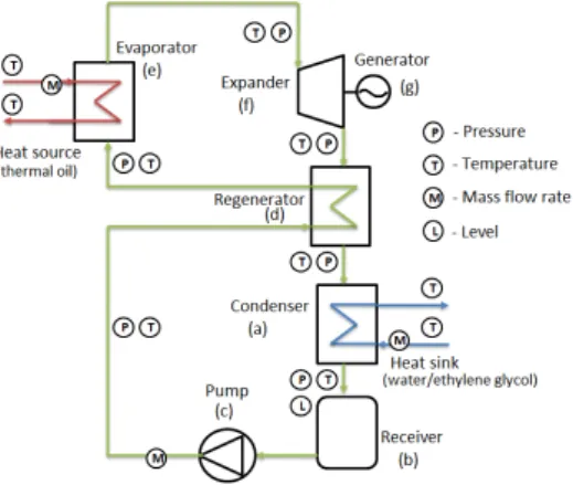
In order to assess the performance of the different developed control strategies, a dynamic model of the ORC system presented in Fig. 1 has been developed in the Modelica language using existent com-ponents from the ThermoCycle library (Quoilin et al., 2014). The developed model is then exported into Simulink/Matlab environment by means of the Functional Mock-Up Interface (FMI) open stan-dard.
Figure 1: Schematic layout of the pilot plant available at Ghent University, campus Kortrijk (Bel-gium)
The system based on a regenerative cycle and solkatherm (SES36) as working fluid, shows a nominal power of 11 kWe. The expander is originally a single screw compressor adapted to run in expander mode. It drives an asynchronous generator connected to the electric grid through a four-quadrant inverter, which allows varying the generator rotational speed (Nexp). During the simulations performed in this paper, the
generator rotational speed is kept constant at 3000 rpm to emulate an installation directly connected to the grid. The circulating pump (Npp) is a vertical variable speed 14-stage centrifugal pump with a maximum
Starting from the bottom of the scheme it is possible to recognize the liquid receiver (b) installed at the outlet of the condenser (a) where the fluid is collected in saturated liquid condition. From the receiver outlet, the fluid is pumped (c) through the regenerator (d) cold side, and the evaporator (e), where it is heated up to superheated vapor, reaching its maximum temperature at the evaporator outlet. The fluid, after being expanded in the volumetric machine (f), enters the regenerator hot side, and then it flows into the condenser (a) to close the cycle.
2.2 Conditions for optimal operation of an ORC unit
In order to optimally operate an ORC unit, two main conditions need to be satisfied: 1) keep the cycle in a safe condition during operation and 2) maximize the net output power. Safe operation of the ORC unit is important as it allows a longer life expectancy in all components. In this concern, an accurate regulation of superheating (ΔTsh), is the main priority since a minimum value of superheating has to be
guaranteed in order to avoid a wet expansion (i.e., formation of liquid droplets at the expander inlet that can damage the expansion machine). The superheating is defined as:
ΔTsh= Texp,su− Tsat,ev (1)
where Texp,suis the temperature measured at the inlet of the expander and Tsat,evthe evaporating
temper-ature, corresponding to the temperature at which the fluid undergoes the phase transition from saturated liquid to saturated vapor at the fixed evaporating pressure psat,ev.
Tsat,ev= f(psat,ev) (2)
where f corresponds to a function that correlates the pressure for the refrigerant.
In order to maximize the output power the evaporating temperature represents the most relevant control variable (Quoilin et al., 2011), which needs to be adapted depending on the heat source conditions (Her-nandez et al., 2015). The main terms to assess the performance of the ORC system are the net output power and the cycle efficiency, which are defined as:
˙
Wel,net= ˙Wexp− ˙Wpump (3)
ηcycle= ˙ Wel,net ˙ Qin,ORC (4)
where ˙Wexp is the expander electrical power, ˙Wpump is the pump electrical power and ˙Qin,ORC is the
thermal power supplied to the ORC system in the evaporator.
2.3 Optimal evaporating temperature
The developed Modelica dynamic model has been used to gain insight on the system’s dynamics, in particular on the relationship between superheating (ΔTsh), evaporating temperature (Tsat,ev), pump speed
(Npp) and expander electrical power ( ˙Wexp). The simulation consists on decreasing the pump speed
Npp from maximum to minimum in small steps. The same experiment is performed for different heat
source conditions, temperature and mass flow, in the ranges Thf = {90, 100, 110, 125}○C and ˙mhf =
{0.5, 0.8, 1.0, 1.5} kg/s, while temperature and mass flow in the heat sink Tcfand ˙mcfwere kept constant
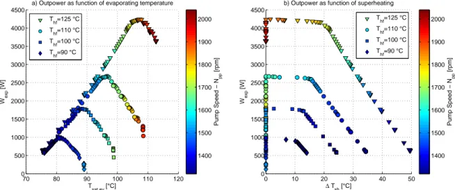
at 15○C and 4 kg/s, respectively. The results for the case of ˙mhf= 1.0 kg/s are depicted in Fig. 2, where
the expander electrical power ˙Wexpis represented as a function of Tsat,evand ΔTsh. Fig. 2a shows how,
for each heat source condition, the expander output power initially grows for increasing evaporating temperature until it reaches a maximum. This is a consequence of the working fluid mass flow that is circulated in the system, see the pump rotational speed value. As the pump speed increases further, two-phase condition appears at the evaporator outlet and a lower output power is registered. Fig. 2b shows the relation between expander output power and superheating level for the same heat source conditions as in Fig. 2a. The power increases as the level of superheating decreases. Notice also that for values of superheating lower than 10○C there is not much gain in the output power. Using the current data it
is then possible to derive a correlation for the optimal evaporating temperature as a function of the heat source conditions:
Tsat,opt= −290.915 + 183.33 ∗ log10(Thf) + 10.636 ∗ ˙mhf (5)
Equation (5) is valid in the range of 0.5≤ ˙mhf≤ 1.5 kg/s and 90 ≤ Thf≤ 125○C given a constant saturation
70 80 90 100 110 120 0 500 1000 1500 2000 2500 3000 3500 4000 4500 T sat,ev [°C] W exp [W]
a) Outpower as function of evaporating temperature
0 10 20 30 40 50 0 500 1000 1500 2000 2500 3000 3500 4000 4500 ∆ T sh [°C] W exp [W]
b) Outpower as function of superheating
Pump Speed − N pp [rpm] 1400 1500 1600 1700 1800 1900 2000 Pump Speed − N pp [rpm] 1400 1500 1600 1700 1800 1900 2000 T hf=125 °C T hf=110 °C T hf=100 °C T hf=90 °C T hf=125 °C T hf=110 °C T hf=100 °C T hf=90 °C
Figure 2: Understanding the operation of an ORC unit. Relationship between output power and a) evaporating temperature and b) superheating for four different heat source conditions Thf =
{90, 100, 110, 125}○C with ˙m
hf= 1.0 kg/s.
3. ADAPTIVE OPTIMIZATION
As presented in section 2.3, in order to maximize the output power it is necessary to find the optimal evaporating temperature for some given heat source conditions. If a dynamic model of the system is known, one can then build a correlation which satisfies also safety conditions. However, there are two drawbacks in this approach: first, a validated dynamic model is not always available and second, there will be modeling errors and consequently a biased correlation.
In this contribution we follow a different approach, by using an Extremum Seeking (ES) algorithm to find the optimal evaporating temperature, which maximizes the output power without the need of a model. Extremum Seeking is a well developed field that addresses the problem of objective value opti-mization when the objective function, its gradient and optimum value are unknown (Ariyur and Krstic, 2003). These techniques are categorized into five main groups: sliding mode ES, neural network ES, approximation based ES, perturbation based ES and adaptive ES. From those the perturbation based ES framework is the most popular method in literature (Ariyur and Krstic, 2003). Since it has proved to be more robust to noise and dynamic effects in the system, thus producing smoother references which decrease the risk of instability (Zhang and Ordonez, 2012).
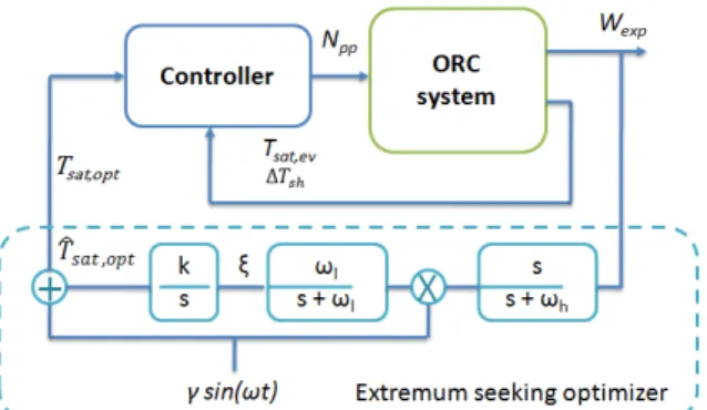
The control structure here proposed is depicted in Fig. 3. A perturbation based ES algorithm is in charge of finding the extremum Tsat,opt that arises from the reference-to-output nonlinear map (i.e., Tsat,ev to
˙
Wexp), while a local feedback controller will keep the system stable at that equilibrium optimal point.
The ES algorithm works as follows: it sends a sine wave to the system as position reference together with an adaptation input:
Tsat,opt= γ sin(ωt) + ˆTsat,opt (6)
with some amplitude γ and modulation frequency ω. The adaptation signal ˆTsat,optshifts the sine wave
towards the gradient direction, thus (6) is the modulation phase of the algorithm. The response of the system to this signal is measured in the objective value ( ˙Wexp). This output is filtered by a high-pass
filter to eliminate the DC component and demodulated by the same sine signal to extract the gradient direction. ξ= Wexp( ωl s+ ωl ) ( s s+ ωh ) (γ sin(ωt)) (7)
Figure 3: Perturbation based extremum seeking algorithm applied to the ORC system. law is computed: ˆ Tsat,opt= ξ k s (8)
where k is a positive constant that specifies the adaptation speed. Since only the DC component of the demodulated signal is needed for gradient calculation, a low pass filter is often used. The amplitude and frequency of the sine wave signal and the cutoff frequencies of the filters are important design parameters. A detailed study of how the design of the perturbation signal affects the performance of the ES algorithm is presented in (Krstic, 2000).
4. MODEL PREDICTIVE CONTROL
A brief introduction to EPSAC algorithm is presented in this section. For a detailed description the reader is referred to (De Keyser, 2003; Hernandez et al., 2015).
4.1 Computing the Predictions
Using EPSAC algorithm, the measured process output can be represented as:
y(t) = x(t) + n(t) (9)
where x(t) is the model output which represents the effect of the control input u(t) and n(t) represents the effect of the disturbances and modeling errors, all at discrete-time index t. Model output x(t) can be described by the generic system dynamic model:
x(t) = f [x(t − 1), x(t − 2), . . . , u(t − 1), u(t − 2), . . .] (10)
Notice that x(t) represents here the model output, not the state vector. Also important is the fact that f can be either a linear or a nonlinear function.
Furthermore, the disturbance n(t) can be modeled as colored noise through a filter with the transfer function:
n(t) =D(qC(q−1−1))e(t) (11)
with e(t) uncorrelated (white) noise with zero-mean and C, D monic polynomials in the backward shift operator q−1. The disturbance model must be designed to achieve robustness of the control loop against unmeasured disturbances and modeling errors (Maciejowski, 2002).
A fundamental step in the EPSAC methodology consists of the prediction. Using the generic process model (9), the predicted values of the output are:
y(t + k∣t) = x(t + k∣t) + n(t + k∣t) (12)
x(t + k∣t) and n(t + k∣t) can be predicted by recursion of the process model (10) and by using filtering
4.2 Computing the optimal control action
A key element in linear MPC is the use of base (or free) and optimizing (or forced) response concepts (Camacho and Bordons, 2004). In EPSAC, the future response can be expressed as:
y(t + k∣t) = ybase(t + k∣t) + yoptimize(t + k∣t) (13)
The two contributing factors have the following origin:
• ybase(t+k∣t) is the effect of the past inputs, the apriori defined future base control sequence ubase(t+
k∣t) and the predicted disturbance n(t + k∣t).
• yoptimize(t+k∣t) is the effect of the additions δu(t+k∣t) that are optimized and added to ubase(t+k∣t),
according to δu(t + k∣t) = u(t + k∣t) − ubase(t + k∣t). The effect of these additions is the discrete time
convolution of ΔU= {δu(t∣t), . . . , δu(t + Nu− 1∣t)} with the impulse response coefficients of the
system (G matrix), where Nuis the chosen control horizon.
The control ΔU is the solution to the following constrained optimization problem:
ΔU=arg min
ΔU∈ RNu N2 ∑ k=N1 [r(t + k∣t) − y(t + k∣t)]2 subject to A.ΔU≤ B (14)
where N1and N2are the minimum and maximum prediction horizons, Nuis the control horizon, r(t+k∣t)
is a future setpoint or reference sequence. The various process input and output constraints can all be expressed in terms of ΔU, resulting in matrices A, B. Since (14) is quadratic with linear constraints in decision variables ΔU, then the minimization problem can be solved by a quadratic programming (QP) algorithm (Maciejowski, 2002; Camacho and Bordons, 2004).
5. SIMULATION RESULTS
The developed ES algorithm is tested in simulation using the proposed EPSAC-MPC strategy and two PI-like strategies. The heat source and heat sink profiles of the ORC system are depicted in Fig. 4. The main variation in the heat source is due to an increase in the temperature (Thf) from 110○C to 120○C. Other
heat source and heat sink variables are rather constant with some small variations around the operating point. 100 200 300 400 110 120 T hf (°C)
Heat source conditions
100 200 300 400
10 15 20 25
Heat sink conditions
T cf (°C) 100 200 300 400 0.5 1 1.5 M hf (kg/s) Time (s) 1002 200 300 400 3 4 Time (s) M cf (kg/s)
Figure 4: Temperature and mass flow rate of the defined heat source and heat sink.
5.1 Low-order model for prediction
MPC requires of a low-order model suitable for prediction. Following a similar approach as the one per-formed in (Hernandez et al., 2015), the model has been identified from the manipulated variable: pump
speed (Npp) to the evaporating temperature (Tsat,ev) and superheating (ΔTsh). Notice that the temperature
Thf in the heat source also influences Tsat,ev and ΔTsh, thus becoming a measured disturbance. As
re-sult we are interested on identifying a system consisting of 2 inputs (one manipulated and one measured disturbance) and 2 outputs.
A linear parametric identification is thus performed in the system using the prediction error minimization method from the data collected using a multisine excitation signal (Ljung, 2007). The identified model presented in (15) is in the form of discrete-time transfer functions for a sampling time Ts= 1 s .
ΔTsh(q) = −0.063q −1+0.059q−2 1−2.44q−1+1.955q−2−0.51q−3Npp(q) + 0.47q −1 1−0.51q−1Thf(q) (15a) Tsat,ev(q) = 0.066q −1−0.063q−2 1−2.42q−1+1.91q−2−0.49q−3Npp(q) + 0.0017q −11−0.0017q−12 1−3.6q−1+4.88q−2−2.95q−3+0.67q−4Thf(q) (15b)
5.2 Performance of ES with constrained EPSAC-MPC strategy
The MPC control objective consists in tracking the optimal setpoint generated by the optimizer (Fig. 3), while keeping the superheating above a desired threshold value to guarantee a safe operation. The control strategy must satisfy these conditions using only one degree of freedom (i.e. pump speed Npp), while
satisfying actuator constraints (Npp,min= 1320 rpm; Npp,max= 2100 rpm; ΔNpp= 100 rpm) and constraints
at the process output (ΔTsh,min= 10○C).
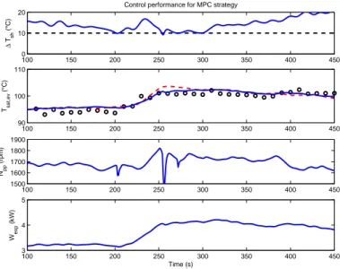
The EPSAC-MPC controller is tuned for horizons N1= 1, N2= 15 and Nu= 1. While the ES optimizer
is tuned for k= 1/38, ωl = 0.02 rad/s, ωh = 0.1 rad/s, γ = 0.05 and ω = 0.06 rad/s. Its performance is
depicted in Fig. 5. 100 150 200 250 300 350 400 450 0 10 20 ∆ Tsh (°C)
Control performance for MPC strategy
100 150 200 250 300 350 400 450 90 100 110 Tsat,ev (°C) 100 150 200 250 300 350 400 450 1500 1600 1700 1800 1900 Npp (rpm) 100 150 200 250 300 350 400 450 3 4 5 Time (s) Wexp (kW)
Figure 5: Control performance of MPC. Dashed-red line represents the ES optimizer while black-circles represents the optimizer obtained from the dynamic model.
Two important elements must be analyzed from results in Fig. 5. First, two optimal evaporating temper-atures are present, one computed using the ES algorithm (dashed red line) and the other (black circles) computed from correlation (5). The ES algorithm is able to adapt properly to the heat source variation, maximizing the output power. Second, it is important to notice that in the time range between 250 and 300 seconds, the controller is not following the setpoint but it rather brings the evaporating temperature closer to the reference computed using correlation (5). This is due to the active constraint in superheat-ing, which causes the controller to take actions in the pump to bring the system in a safer regime (i.e., ΔTsh> 10○C). Remember that equation (5) was computed to ‘guarantee’ superheating will remain above
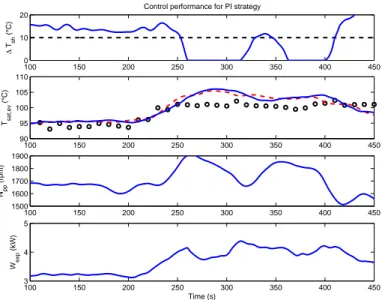
5.3 Performance of ES with PI-like strategies
The EPSAC-MPC strategy is replaced by two PI-like controllers, in order to compare the performance. The first strategy consists on a PI controller used to track the reference given by the ES optimizer. The second strategy consists in using a PI controller to track the optimal evaporating temperature unless su-perheating goes below the threshold value of 10○C, in which case a second PI controller for superheating
with reference at (ΔTsh,ref= 10○C) is activated, thus bringing the system back into a safer regime.
100 150 200 250 300 350 400 450 0 10 20 ∆ Tsh (°C)
Control performance for PI strategy
100 150 200 250 300 350 400 450 90 95 100 105 110 Tsat,ev (°C) 100 150 200 250 300 350 400 450 1500 1600 1700 1800 1900 Npp (rpm) 100 150 200 250 300 350 400 450 3 4 5 Time (s) Wexp (kW)
Figure 6: Control performance for a PI strategy. Dashed-red line represents the ES optimizer while black-circles represents the optimizer obtained from the dynamic model.
100 150 200 250 300 350 400 450 0 10 20 ∆ Tsh (°C)
Control performance for Switching PI strategy
100 150 200 250 300 350 400 450 90 100 110 Tsat,ev (°C) 100 150 200 250 300 350 400 450 1500 1600 1700 1800 1900 Npp (rpm) 100 150 200 250 300 350 400 450 3 4 5 Time (s) Wexp (kW)
Figure 7: Control performance for a switching PI strategy. Dashed-red line represents the ES optimizer while black-circles represents the optimizer obtained from the dynamic model.
The result for the single PI strategy is depicted in Fig. 6. The ES optimizer (dashed red line) adapts the reference to the local PI controller, finding the point which maximizes the output power. As known from section 2.3 and Fig. 2 this maximum corresponds to zero superheating values. Since this strategy does not supervise superheating, once the controller tracks this reference the system reaches zero super-heating, decreasing the generated power Wexpas observed at time 250 to 300 seconds and 350 to 400
Next it is evaluated the performance of the switching PI strategy as depicted in Fig. 7. In this case the controller tracks the reference generated by the ES optimizer (dashed red line); but once it detects superheating values below 10○C, the PI controller for superheating becomes active. Thus avoiding that
the organic fluid is in two-phase (i.e., gas and liquid phase) which would decrease the performance of the system as observed for the single PI strategy. Although the switching mechanism avoids superheating going to zero, it still reaches values near 5○C and requires of more aggressive control actions which
increases power consumption in the pump compared to the EPSAC-MPC. Nevertheless, its simplicity is still remarkable.
5.4 Discussion of the obtained results
Although safety is highly important for Rankine cycles, it is also interesting to look into the net energy produced. Using results from Fig. 5 and Fig. 7, the net output power is calculated using (3). These values of net output power are further integrated over time to obtain the energy produced for each of the control strategies.
Taking the switching PI as a reference (100%), the EPSAC-MPC strategy allows increasing the net energy
production by 21%. This is due to a better handling of the constraints, thus operating the system closer
to the constraint for superheating while requiring a lower control effort (i.e., less power consumption in the pump) as observed in the results during the time from 250 to 300 seconds.
In an industrial context the single PI strategy solely is not safe to be applied, therefore its output power is not computed.
6. CONCLUSIONS
In this contribution a two layer control structure to achieve constrained optimal operation of an organic Rankine cycle unit for waste heat recovery applications is proposed. First, an optimizer based on a perturbation based extremum seeking algorithm is designed and implemented, to find the near-to-optimal evaporating temperature which maximizes energy production. Second, a constrained model predictive controller is implemented to track the optimal evaporating temperature given by the optimizer, while keeping the safety limit for superheating. Finally, the performance of the resulting loop is compared to PI control strategies. It is shown that a single PI cannot guarantee safety conditions, therefore a switching PI is proposed, resulting in a safer operation compared to a single PI but less effective compared to model predictive control since it violates safety limit for superheating and produces a lower net output power.
Future work will include the development of a multivariable control strategy by making use of the ex-pander speed, as an additional manipulated variable.
NOMENCLATURE
ORC Organic Rankine Cycle
WHR Waste Heat Recovery
MPC Model Predictive Control
EPSAC Extended Prediction Self-Adaptive Control PI Proportional-Integral Control
ES Extremum Seeking
˙
m Mass flow rate (kg/s)
˙
W Power (W)
N Rotational speed (rpm)
p Pressure (Pa)
Subscript Greek letter
el Electric η Efficiency
ev Evaporator γ Amplitude perturbation in ES algorithm
exp Expander α Time constant reference trajectory in MPC
pp Pump
REFERENCES
Ariyur, K. and Krstic, M. (2003). Real-Time optimization by Extremum-Seeking Control. John Wiley & sons.
Camacho, E. F. and Bordons, C. (2004). Model Predictive Control, volume 405 pages. Springer-Verlag, London„ 2nd edition.
De Hann, D. and Guay, M. (2005). Extremum-seeking control of state-constrained nonlinear systems.
Automatica, 41:pp. 1567–1574.
De Keyser, R. (2003). Model based Predictive Control for Linear Systems, chapter invited in UNESCO Encyclopaedia of Life Support Systems (EoLSS). Article contribution 6.43.16.1, Eolss Publishers Co Ltd, Oxford, 35p.
Hernandez, A., Desideri, A., Ionescu, C., Quoilin, S., Lemort, V., and De Keyser., R. (2015). Experi-mental study of predictive control strategies for optimal operation of organic rankine cycle systems. In Proceedings of the European Control Conference (ECC15), Linz, Austria.
IEA (2010). Industrial excess heat recovery technologies & applications. Technical report, Technical report, Industrial Energy-related Technologies and Systems (IETS).
Krstic, M. (2000). Performance improvement and limitations in extremum seeking control. systems and
control letters, vol. 39:pp. 313–326.
Ljung, L. (2007). System identification: theory for the user. Prentice-Hall.
Maciejowski, J. (2002). Predictive Control: With Constraints. Pearson Education. Prentice Hall. Quoilin, S., Aumann, R., Grill, A., Schuster, A., and Lemort., V. (2011). Dynamic modeling and optimal
control strategy for waste heat recovery organic rankine cycles. Applied Energy, Vol. 88:2183–2190. Quoilin, S., Desideri, A., Wronski, J., Bell, I., and Lemort., V. (2014). Thermocycle: A modelica library for the simulation of thermodynamic systems. In Proceedings of the 10th International Modelica
Conference, Lund, Sweden.
Wei, D., Lu, X., Lu, Z., and Gu., J. (2007). Performance analysis and optimization of organic rankine cycle (orc) for waste heat recovery. J. Energy Conversion and Management, Vol. 48:1113–1119. Zhang, C. and Ordonez, R. (2012). Extremum-Seeking Control and Applications. A Numerical
Optimization-Based Approach. Advances in Industrial Control. Springer-Verlag. ACKNOWLEDGEMENT
The results presented in this paper have been obtained within the frame of the IWT SBO-110006 project The Next Generation Organic Rankine Cycles (www.orcnext.be), funded by the Institute for the Pro-motion and Innovation by Science and Technology in Flanders. This financial support is gratefully acknowledged.