Automatic time stepping algorithms for implicit numerical simulations of blade/casing interactions.
Abstract – An automatic time step size determination for non-linear problems, solved by implicit schemes, is presented. The time step calculation is based on the estimation of the integration error. This estimation is calculated from the acceleration difference. It is normalised according to the size of the problem and the integration parameters. This time step control algorithm modifies the time step size only if the problem has a long time physical change. On the other hand, Hessian matrix can be kept constant for several iterations however the problem is non-linear. According to the fact that the time step size is constant for some time step, the Hessian matrix shouldn’t be recalculated for each time step. A criterion selecting if Hessian matrix must be calculated or not is developed. Finally, a criterion of iterations divergence is also proposed. It avoids the determination, by the user, of a maximal iterations number. The iterations number is the smaller. Industrial numerical examples are presented that demonstrated the performances (precision and computational cost) of the algorithms.
NOTATION.
tn time after the time step number n h time step size
q vector of nodal positions
qn vector of nodal positions at time tn after convergence of the iterations qin vector of nodal positions at time tn after the iteration number i q0n vector of nodal positions at time tn after prediction
qo vector of nodal positions at initial time.
M mass matrix
Fint vector of internal forces Fext vector of external forces ∃ first Newmark parameter ( second Newmark parameter
∀M first free parameter balancing sampling time around [tn, tn+1] for averaging inertia terms
∀F second free parameter balancing sampling time around [tn, tn+1] for averaging forces
∗ accuracy tolerance on the non-dimensional residue Ct tangent damping matrix
Kt tangent stiffness matrix St Hessian matrix
R residue of the equation of motion
r non-dimensional residue of the equation of motion Τ pulsation for a one degree of freedom linear system Σ non-dimensional pulsation (Τh)
ε integration error for a one degree of freedom linear system e integration error for the system
PRCU tolerance of the integration error
RAT factor multiplying the time step size between two steps INTRODUCTION.
Non-linear dynamic problems can be solved with two kind of time-stepping algorithms: explicit or implicit. For an explicit code, solution at time tn depends only on solution at time tn-1. For an implicit code, solution at time tn
depends on solution at time tn-1 but also at time tn. System is then solved with iterations. On the other hand, for
an implicit algorithm the time step size can be longer than for an explicit algorithm. However the cost for a time step is higher for an implicit scheme, the time step number is smaller and the total time of calculation is often more interesting than for an explicit scheme. If the time step size is chosen too small, the calculation cost is very expensive. If it is chosen too big, the integration is not accurate enough or the iterations diverge. Therefor, time step size must be correctly calculated. According to the fact that the problem evolves with time, time step size must be adapted with this evolution. An automatic time step determination is then the only solution to solve accurately the problem in a short calculation time. For an industrial problem that has a large number of degrees of freedom, the most expensive operation of an implicit code is the inversion of the Hessian Matrix. For non-linear problems, the Hessian matrix changes at each iteration. The Newton-Raphson iterations can sometimes converge when using the old inverted matrix. But this inverted matrix must be frequently recalculated otherwise the iterations diverge. This inversion occurs generally at begin of each time step and for some iteration selected
by the user. But, if the Hessian matrix is not regularly inverted, problem diverges and if the inversion occurs too frequently, the problem becomes too expensive. According too the evolution of the problem with time, an automatic determination selecting if the inverted Hessian matrix must be recalculated or not, can reduce the total calculation cost. When the Newton-Raphson iterations diverge, the time step is rejected and the time step size is reduced. A problem is to determinate when the iterations diverge. Usually a maximum number of iteration is defined. If this number is too small a time step can be rejected however the problem slowly converges. If this number is chosen too big, some iteration are needlessly calculated when the divergence occurs. It is then interesting to determinate if divergence occurs in accordance with the residue evolution. The maximum number of iteration is more difficult to be correctly determinate when the inverted matrix is not calculated at each iteration. Indeed, this number depends on how frequently the inverted matrix is calculated. This paper proposes an automatic time step control algorithm based on the measure of the integration error. This algorithm modifies the time step size only if durable physical change occurs in the problem evolution. An automatic determination choosing if the Hessian matrix is recalculated is also proposed. This determination is based on residue evolution with iterations. Finally, a divergence criterion based on this residue evolution is implemented. Industrial numerical examples are then calculated with these new algorithms.
NUMERICAL INTEGRATION OF TRANSIANT PROBLEMS WITH AN IMPLICIT CODE. The equations of motion of a non-linear structure, discretized in finite elements, can be write:
(
,)
−(
,)
= 0+ F q q F q q
q
M && int & ext & (1)
First term of equation (1) is the vector of inertial terms. Second one is the vector of internal forces. This term is non-linear according to the geometrical non-linearity and plastic deformations. Last term is the vector of external forces. The non-linearity can be due from contact modelling, imposed displacements…
The most general scheme for implicit integration, is based on averaged accelerations between time tn and tn+1. If positions and velocities at time tn are knew, positions and velocities at times tn+1 can be written:
⎪ ⎪ ⎩ ⎪⎪ ⎨ ⎧ + − + = + − + + = + + + + q h q h q q q h q h q h q q n n n n n n n n n && && & & && && & 1 1 1 2 2 1 ) 1 ( ) 2 1 ( γ γ β β
(2)
Numerical dissipation is introduced in relation (1). This numerical dissipation damped numerical high frequency modes that occur for constrained problems. A general form was introduced by Chung and Hulbert, and (1) was rewritten [1]:
(3) ⎪⎩ ⎪ ⎨ ⎧ = − + − − + + − + + + + + 0 )] , ( ) , ( [ )] , ( ) , ( )[ 1 ( ) 1 ( 1 1 1 1 1 q q F q q F q q F q q F q M q M n n ext n n int F n n ext n n int F n M n M & & & & && && α α α α
Unconditional stability requires ( ∃ 0.5 - ∀M + ∀F , ∀M # ∀F # 0.5 and ∃ ∃ 0.25 + (∀F - ∀M) / 2. The Hessian matrix for iteration number i+1 is defined by:
M h C h K St F t t ²M ) 1 ( ) )( 1 ( −α + βγ + −βα =
(4)
where the tangent matrix are defined by:
(
)
(
)
⎪ ⎪ ⎪ ⎩ ⎪⎪ ⎪ ⎨ ⎧ ⎥ ⎦ ⎤ ∂− ∂ = ⎥ ⎦ ⎤ ∂− ∂ = + + + + q q q q i n i n i n i n q F F C q F F K ext t ext t & & & 1 1 1 1 , int , int (5))] , ( ) , ( [ )] , ( ) , ( )[ 1 ( ) 1 ( 1 1 1 1 1 q q F q q F q q F q q F q M q M R n n ext n n int F i n i n ext i n i n int F i n M i n M & & & & && && − + − − + + − = α α + α α + + + + (6)
Using relations (4) and (6), iterative solve of system (2) and (3) can be write as:
St)q = -R (7)
Iterations stopped when non-dimensional residue r becomes lower than the accuracy tolerance ∗. Therefore the following relation is verified:
< δ + = F F R r int ext (8)
AUTOMATIC TIME STEP SIZE CONTROL. Bibliography studies.
Ponthot [1] proposes an optimal number of iterations. If the number of iteration exceeds this optimal number, time step size is reduced. On the other hand, if the number of iterations is lower, time step size is augmented. Givoli and Henisberg [2] propose to modify the time step size to keep the displacement difference, between two successive times, lower than a limit. Geradin [3] estimates the integration error from the accelerations and the inertial forces difference between two successive times multiplied by the square of time step size. This error is divided by a constant depending on the initial positions and by a constant that is the average error for a one degree of freedom linear system. The error must be lower than a tolerance. If the error is higher, the time step is rejected and the time step size is divided by two. If the error is lower than tolerance but higher than a half tolerance, time step is divided by the rapport between the error and the half tolerance to the power a third. If the error is lower than tolerance divided by sixteen, the time step size is multiplied by two. For Cassano and Cardona [4], the times step control is the same than for Geradin but the error is calculated only from the acceleration difference and is not divided by a constant depending on the initial positions but by a term that evolves with positions. Hulbert and Jang [5] estimate the error from the accelerations difference multiplied by the square of time step size. Error is divides it by a term that depend on the position difference. Time step control is characterised by two tolerances (TOL1 and TOL2) and by a counter whose maximal index is LCONT. If the error is higher than TOL2 then the step is rejected and time step size is reduced. If error is lower than TOL2 and higher than TOL1 time step is accepted and time step size is kept constant. If the error is lower than TOL1 then time step is accepted. If it occurs successively LCOUNT times then the times step size is augmented. The counter is introduced to avoid undesirable change in time step size due to periodic nature of the local error. Dutta and Ramakrishnan [6] also calculate the error from the acceleration difference multiplied by the square of the time step size. It is made non-dimensional by dividing it by the maximum norm of the position vector, for the previous time step. The time interval is divided in sub-domains. In each sub-domain there is a lot of time step that has constant size. Once each time step of a sub-domain is calculated, an average error is calculated. Time step size for next sub-domain is then calculated from this average error.
In this paper the automatic control scheme is based on the algorithm proposed by Geradin. Nevertheless, due to the non-linear characteristic of the problems, we will assumes that time step size react only on evolution in physical mode and not on numerical mode. Change in time step size will also occurs only if the new time step size can be kept constant for several time steps.
Error calculation.
This algorithm is implemented in the module MECANO de SAMCEF. Calculation of the integration error is the one that exists in MECANO. It was the one developed by Geradin. Error is then [II]:
( )
[
]
[
(
)
]
2 1 2 1 0 0 2 6 q M q q M q h e T T k && && ∆ ∆ Ω = ε (9)In this expression, q0 is the initial vector of positions and ε (Σ) is the average error for a one degree of freedom linear system with pulsation Τ, time step h and non-dimensional pulsation Σ=Τh. It is evaluated for Σk=0.6. This
value gives correct results for a one-degree of freedom linear system. Resolving (3) and (2) for a one-degree linear system, ε take the following expression:
( )
[
(
)
(
)
β]
α α π α ε Ω − + − Ω + Ω − = Ω 2 2 3 1 1 3 4 1 1 F M F (10) Remarks:- Expression (9) come from the troncature error of the equation (2). Indeed, the error is on the third order and is write e = O
( ) (
h3&q&& ≈ Oh2∆q&&)
. Geradin [2] demonstrates than for a linear multi degree of freedom system this expression can be write as (9). However for non-linear system no advantage appears of replacing the acceleration difference by a term depending on the accelerations and the inertial forces difference as in (9).- Error is divided by expression (10) evaluated in Σk to have an estimation of the error that not
depends of the integration parameters. Time step size control.
The error calculated must be on the order than a tolerance the user gives “PRCU”. A low “PRCU” gives a good accuracy but a long calculation time. A higher “PRCU” gives a lower time calculation and a lower accuracy. On the other hand, if “PRCU” is high the time step size can give a error lower than “PRCU” but can be not small enough to allow the iterations to converge. Therefore, if a problem of convergence appears, the algorithm reduces “PRCU”.
If the iterations converge, the algorithm tries to adjust the time step size to have an error equal at an half “PRCU”. There exist three possibilities:
- The error is bigger than “PRCU/2”. It is considered to be too high. To assure a good accuracy time step size must be reduced.
- The error is smaller than a limit “SEUIL”. It is considered to be too small. To assure a reduced calculation cost, time step size must be augmented.
- The error is in the interval [SEUIL; PRCU/2]. The time step size assures a good accuracy in a relatively low calculation cost. Time step size is kept constant
Let us first examine the problem of a too high error. Time step size must therefore be reduced. But to avoid needlessly changes in time step, we will assume that the variation of the integration error is due to a durable and physical evolution in the problem. Time step is then reduce only if there are a number (CO) of successive time steps whose integration error is upper PRCU/2. This number “CO” can be take equals at three. The factor that reduces the time step size depends on the maximum error (ERRO) of the “CO” successive time steps. Geradin demonstrates than for a linear one degree of freedom system, the factor multiplying the time step size needed to reduced the error from e to PRCU/2 can be write:
[
]
1η2e
PRCU
RAT = , 00 [2, 3] (11)
For non-linear systems 0 can be out of this interval. To assure the time step size is sufficiently reduced, 0 is taken smaller than two. Factor that finally multiplies time step size is RAT=[0.5 PRCU/ERRO]2/ 3. A counter is introduced. But if there is a rapid change in the physical problem (impact,…) the time step is not immediately adapted. Therefore, if the error “e” is upper PRCU, the time step size is immediately multiplied by RAT=[0.5
PRCU/e]2/ 3. If the error “e” is bigger than a limit “REJL”, time step size is multiplied by RAT=[0.5 PRCU/e]2/ 3
but time step is rejected. REJL can be taken equal at 1.5 PRCU.
Now let us examine the problem of a too small error. Time step size could be augmented without degrading the solution. To avoid needlessly time step size change, another counter is introduced. If “CT” successively time step give an error lower then the limit SEUIL, then time step size is augmented. ERRT is the maximal error of those CT steps. To assure the time step size is not too augmented, 0 from equation (11) is taken bigger than 3. The factor multiplying time step size is finally RAT=[0.5 PRCU/ERRT]1/ 5. A problem due to the introduction of a counter occurs when the problems becomes more smooth (external forces diminishes…). Indeed, SEUIL must be taken small (PRCU/16 e.g.) and CT relatively big (5 e.g.) to assure good accuracy. In those conditions, time step size augments slowly. To reduce calculation cost, SEUIL can augment and CT can decrease when time step size is augmented. SEUIL can be multiplied by 1.3 and CT reduced to 4 first and to 2 next. Once a time step size
is reduced SEUIL and CT become equal at respectively PRCU/16 and 1.3 again. In some problems (translation at constant velocities), error becomes nil. To avoid a division by zero, ERRT is limited by SEUIL PRCU / 10. CRITERION SELECTING THE RECALCULATION OF THE INVERTED HESSIAN MATRIX. For non-linear problems, if the Hessian matrix is not recalculated and inverted, the convergence of Newton-Raphson iterations is less quick than if Hessian matrix is recalculated and inverted at each iteration. For some step divergence could also occur. Therefore, the criterion must consider two facts:
- Convergence of the iterations must be assured.
- Not recalculate Hessian matrix must reduce total calculation cost. Indeed, a problem with a little number of degree of freedom and with strong non-linearity can converge with a few iteration when Hessian matrix is recalculated at each iteration but converge with more iteration when the Hessian matrix is not recalculated. When the number of degree of freedom is reduced, an iteration without recalculation is not very less expensive. Total cost is then reduced when Hessian matrix is often recalculated. On the other hand, if the problem has a large number of degree of freedom en only some elements non-linear, then not recalculate the Hessian matrix can reduced the calculation cost. Evolution of non-dimensional residue r (relation (8)) could indicate if the problem converges or not. While r decrease, iterations converge even if the Hessian matrix is not recalculated and not inverted. An indication of how it could be interesting not to recalculate the Hessian matrix is the ratio “VALREF” between the time needed for an iteration with recalculation and a iteration without recalculation. This ratio indicates how much iteration without recalculation could advantageously replace an iteration with recalculation. This value VALREF is an entire limited between 2 and 15.
The developed algorithm is the following:
- Hessian matrix is recalculated at the first iteration if the time step size is changed. Indeed, St depends on h (relation (4)). No convergence is possible if St is not recalculated.
- If the number of the iteration is greater than VALREF, this iteration is made with recalculation of the Hessian matrix. Then, iterations occur without recalculation only if it is less expensive.
- If the number of the iteration is lower than VALREF, Hessian matrix is recalculated only if the non-dimensional residue r is not be divided by a ration chosen equal at RAPRES = VALREF / 10 0 [0.75, 0.95].
- If the non-dimensional residue has not been divided by RAPRES, next iteration need then recalculation of the Hessian matrix. But ideally, this iteration does not take as initial values ( ) the values at the end of the previous iteration, but the value at the end of last iteration who has converged. Some divergences of the iteration are then avoided. For practical reasons, implementation in MECANO was not possible with this last remark. Then the next solution has been adopted. If the non-dimensional residue has not been divided by RAPRES, the next iteration occurs with recalculation and the initial values are the prediction values.
q q q, &, &&
- If an iteration, with a number lower than VALREF and upper than one, with recalculation of the Hessian matrix occurs, all the next iterations of this step occurs with recalculation. Convergence is then assured.
- If last iteration of the previous time step has needed a recalculation of the Hessian matrix, first iteration of the present step occurs with recalculation.
This algorithm avoids some needlessly recalculations and inversion of the Hessian matrix. For problems strongly non-linear with a little number of degree of freedom, this algorithm is at worst also expensive than an algorithm with recalculation at each iteration. For problems with more degree of freedom, this algorithm is less expensive than an algorithm that the user decides the number of the iterations with recalculation. In fact, this algorithm allows a lot of iteration without recalculation when possible and recalculates frequently the Hessian matrix when needed.
CRITERION OF DIVERGENCE.
Usually, the user gives a maximum number of iteration. If after this number the non-dimensional residue r is not lower than the tolerance ∗, the time step is rejected and the time step size is divided. But when the residue r decrease slowly, the maximum number of iteration is exceeded before r becomes lower than ∗. On the other hand, iteration can diverges after a few numbers of iterations. Next iterations are then needlessly. Finally if we accept the problem to be resolved without recalculation of the Hessian matrix, the number of iterations is higher
than when frequently recalculation occurs. A solution consists to consider than divergence occurs if after 5 iterations with recalculation, the non-dimensional residue is not divided by two.
NUMERICAL EXEMPLES.
The three algorithm are implemented in the dynamic module MECANO of SAMCEF [9]. Actually, time step size in MECANO is choosen with the scheme of Geradin. The user defines the number of the iteration with recalculation of the Hessian matrix and the maximum number of iterations. With the actual algorithm, recalculation occurs at the first iteration of time step according to the fact that time step size can change. Two industrial problems from SNECMA are calculated with the old and the new algorithm. These problems cannot be precisely described for confidential reasons. For the same reasons, axes are not graduated. Nevertheless we are authorised to tell that problems where three dimensional models with some thousands of degree of freedom. Some elements are non-linear simulating contacts, rupture… Problems are also non-stationary. When comparing the new and the old algorithms, precision parameters (∗, PRCU) are taken identically. For the old algorithm, the iterations number with recalculation of the Hessian matrix are chosen to minimise the total cost calculation. Some attempts are necessary to define these parameters for having a low cost without divergence of the problems.
Case 1
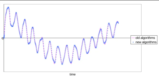
This problem is solved with the old algorithms and the new ones. In the two cases, tolerance ∗ on non-dimensional residue r is taken equal at 1E-3. Tolerance PRCU on integration error is taken equal at 1E-3. Initial time step size is the same. With the old algorithms, there is recalculation of the Hessian matrix for iteration 1, 3, 6, 7, 8, 9… Parameters of integration are the same for both methods (∀M=0, ∀F=0.1). Figure 1 is moving for a
degree of freedom of case 1. New algorithms give a solution nearly equal as the old ones. Figure 2 is the energy balance of case 1. The energy balance is the potential energy plus kinetic energy min external forces work. If this balance is positive, energy appears with times, the integration is non-stable. If this balance is negative, energy disappears. It could be due to physical dissipation or numerical dissipation. If numerical dissipation is too high, the integration is not accurate. On Figure 2, we see that dissipation with new algorithms is a few lower (0.5%) than with old algorithms. New algorithms give then a good accuracy. Calculation costs are given on Figure 3. News algorithms decrease the CPU time to 40%.
time
q old algorithms
new algorithms
-0,7 -0,6 -0,5 -0,4 -0,3 -0,2 -0,1 0 0,1 tim e energy balance (%) old algorithm s new algorithm s
Figure 2 - Energy balance of case 1.
CPU old algorithms
new algorithms
Figure 3 - Calculation costs of case 1. Case 2.
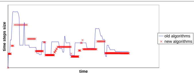
This problem is solved with the old algorithms and the new ones. In the two cases, tolerance ∗ on non-dimensional residue r is taken equal at 1E-4. Tolerance PRCU on integration error is taken equal at 1E-3. Initial time step size is the same. With the old algorithms, there is recalculation of the Hessian matrix for iteration 1, 3, 5, 6, 7, 8… Parameters of integration are the same for both methods (∀M=0, ∀F=0.1). Figure 4 represents force
evolution for a degree on freedom of case 2. The news algorithms give the same solutions than the old ones. Figure 5 shows the evolution of time step size. With new algorithm of time step control, the time step size is constant during longer periods. Less greater times steps are then rejected and recalculations of Hessian matrix because time step size has changed can be avoid. Figure 6 gives the calculation time needed for both methods. New algorithms reduce calculation time to 60%.
time
F
old algorithms new algorithms
time
time steps size
old algorithms new algorithms
Figure 5 - Time step size evolution for case 2.
CPU
old algorithms
new algorithms
Figure 6 - Calculation costs for case 2.
CONCLUSIONS.
A new time step size control algorithm was presented. This algorithm is based on the measure on an integration error. By introducing counter, time step size is modified only for physical and durable variations in the dynamic problems. But for a sudden change as an impact or a contact, integration error increases in a time step and the algorithm reduces instantaneously the time step size. By modifying the limit under the time step could be augmented, if the problem becomes smoother, times step size can increase rapidly. This algorithm gives then a good accuracy with a low calculation time and a constant time step for long period. If problem of convergence occurs, tolerance on integration error is reduced to adapt time step with convergence problems. Some rejected time steps are then avoided.
Next, an algorithm deciding if the Hessain matrix must be recalculated was proposed. This algorithm recalculates the Hessian matrix only if it is necessary to converge. If not, the old Hessian matrix is used for iterate and calculation time is reduced.
Finally a criterion of divergence was implemented. It considered that problem does not converge if non-dimensional residue does not decrease when iterating. A lot of needlessly are then avoided.
The proposed algorithms were implemented in MECANO of SAMCEF, and two industrial problems were calculated. The solutions with the new algorithms are also accurate than with the existing algorithms, but calculation costs were reduced to an order of 50%.
BIBLIOGRAPHIE.
Traitement unifié de la mécanique des milieux continus solides en grandes transformations par la méthode des éléments finis
Thèse présentée en vue de l’obtention du titre de Docteur en Sciences Appliquées de l’Université de Liège (1994-1995)
[2] GIVOLI D. and HENISBERG I. A simple times-step control scheme
Communication In Numerical Methods In Engineering, Vol 9, 873-881 (1993) [3] GERADIN Michel (LTAS)
Analyse, simulation et conception de systèmes polyarticulés et structures déployables
Cours IPSI Paris, 11-13 mars 1997 [4] CASSANO A. and CARDONA A.
A comparaison between three variable-step algorithms for the integration of the equations of motion in structural dynamics
Latin American Research 21, 187-197 (1991) [5] HULBERT G.M. and JANG I.
Automatic time step control algorithms for structural dynamics
Computer Methods In Applied Mechanics and Engineering 126, 155-178 (1995) [6] DUTTA A. and RAMAKRISHNAN C.V.
Accurate computation of design sensitivities for structures under transient dynamic loads using time marching scheme
International Journal For Numerical Methods In Engeneering 41, 977-999 (1998) [7] GERADIN M. and RIXEN D.
Théorie des vibrations. Application à la dynamique des structures.
Masson (1993)
[8] HUGHES Thomas
The finite element method (linear static and dynamic finite element analysis), Prentice-Hall Internationnal Editions, 1987
[9] SAMTECH,