Prediction of Miscible Mixtures Flash-point from UNIFAC group contribution methods

O

pen

A

rchive

T

oulouse

A

rchive

O

uverte (

OATAO

)

OATAO is an open access repository that collects the work of Toulouse researchers and makes it freely available over the web where possible.

This is an author-deposited version published in: http://oatao.univ-toulouse.fr/ Eprints ID: 4498

To link to this article:

http://dx.doi.org/10.1016/j.fluid.2010.10.007

To cite this version: Liaw, Horng-Jang and Gerbaud, Vincent and Li, Yi Hua ( 2011) Prediction of Miscible Mixtures Flash-point from UNIFAC group contribution methods. Fluid Phase Equilibria, vol. 300 (n° 1-2). pp. 70-82. ISSN 0378-3812

Any correspondence concerning this service should be sent to the repository administrator: staff-oatao@inp-toulouse.fr

Prediction of Miscible Mixtures Flash-point from UNIFAC group

contribution methods

Horng-Jang Liaw a, Vincent Gerbaud b,c, Yi-Hua Li a

a

Department of Occupational Safety and Health China Medical University

Taichung, Taiwan, R.O.C. b

Université de Toulouse, INP-ENSIACET, UPS, LGC (Laboratoire de Génie Chimique), 4 allée Emile Monso - BP 84234 - 31432 TOULOUSE cedex 4 – France

c

CNRS, LGC (Laboratoire de Génie Chimique), 4 allée Emile Monso - BP 84234 - 31432 TOULOUSE Cedex 01 – France

Address correspondence to: Dr. Horng-Jang Liaw

Department of Occupational Safety and Health China Medical University

91 Hsueh-Shih Rd., Taichung, Taiwan Tel: 886-4-22053366 ext. 6209

Fax: 886-4-22030418

Prediction of Miscible Mixtures Flash-point from UNIFAC group

contribution methods

Horng-Jang Liaw a, Vincent Gerbaud b,c, Yi-Hua Li a

a

Department of Occupational Safety and Health, China Medical University 91 Hsueh-Shih Rd., Taichung, Taiwan

b

Université de Toulouse, INP-ENSIACET, UPS, LGC (Laboratoire de Génie Chimique), 4 allée Emile Monso - BP 84234 - 31432 TOULOUSE cedex 4 – France

c

CNRS, LGC (Laboratoire de Génie Chimique), 4 allée Emile Monso - BP 84234 - 31432 TOULOUSE Cedex 01 – France

ABSTRACT

Flash point is one of the most important variables used to characterize fire and explosion hazard of liquids. This paper predicts the flash point of miscible mixtures by using the flash point prediction model of Liaw and Chiu (J. Hazard. Mater. 137 (2006) 38-46) handling non-ideal behavior through liquid phase activity coefficients evaluated with UNIFAC-type models, which do not need experimentally regressed binary parameters. Validation of this entirely predictive model is conclusive with the experimental data over the entire flammable composition range for twenty four flammable solvents and aqueous−organic binary and ternary mixtures, ideal mixtures as well as Raoult’s law negative or positive deviation mixtures. All the binary-mixture types, which are known to date, have been included in the validated samples. It is also noticed that the greater the deviation from Raoult’s law, the higher the probability for a mixture to exhibit extreme (minimum or maximum) flash point behavior, provided that the pure compound flash point difference is not too large. Overall, the modified UNIFAC-Dortmund 93 is recommended, due to its good predictive capability and more completed database of binary interaction parameters. Potential application for this approach concerns the classification of flammable liquid mixtures in the implementation of GHS.

1. Introduction

Safety in the usage and storage of flammable and combustible liquid mixtures is much needed as dramatic accidents regularly occur, such as a series of explosions of essential oils in 2003 and the Shengli illegal dumping event in 2006 in Taiwan [1-3]. In 2007, a gasoline tanker crashed and burst into flames near the San Francisco-Oakland Bay Bridge, resulting in a stretch of highway melted and collapsed [4,5], highlighting the importance of safe transportation for flammable and combustible liquids. The fire and explosion hazard of liquids is primarily characterized by their flash point [6]. The flash point is defined as the temperature determined experimentally at which a liquid emits sufficient vapor to form a combustible mixture with air [7].

The United Nations encouraged the worldwide implementation of the GHS (Globally Harmonized System of Classification and Labeling of Chemicals) in 2008, and within it, the flash point of mixtures is the critical reference property in the classification of flammable liquids. Unfortunately, mixture flash-point data is scarce and deriving such data using test instruments is a time-consuming work, both may explain the decision of the EC (European Community) CLP (Classification, Labeling and Packaging) to delay the classification of mixtures until 2015 [8].

Since the cost of deriving flash-point data from test instruments is very high, NT$20,000/US$600 per sample in Taiwan, several alternative models for predicting the flash points of different type of mixtures have been proposed, especially for miscible mixtures [1-3, 6, 9-16]. Models based on the assumption of ideal solutions [6, 9-11] show limitations when applied to the non-ideal mixtures, which are the most frequent ones. Models taking into account the non-ideality of the solution through liquid-phase activity coefficients have a wider application range and predicted efficiently the flash point of miscible mixtures [1-3, 12, 13, 15, 16]. The non-ideality of the liquid phase is accounted for by liquid-phase activity coefficients by means of thermodynamic models. The frequently used NRTL, Wilson and UNIQUAC thermodynamic models, require binary interaction parameters regressed on experimental data, and are thus often missing due to the vast combination of possible mixtures. By contrast, predictive models such as the UNIFAC models [17, 18] do not need experimental binary interaction parameters. Instead, chemical group contributions obtained from a large database are summed to evaluate the interaction parameters, and can be used to compute binary mixture flash-points [15, 19].

The original UNIFAC model [17, 18] splits the activity coefficient into a combinatorial and a residual part. In order to improve the performance of the original UNIFAC model in the prediction of vapor−liquid equilibrium (VLE),

liquid−liquid equilibrium (LLE), and excess enthalpies, many modification in the combinatorial, as well as the residual, term of this model have been suggested [20−25].

Gmehling and Rasmussen (1982) were the first to calculate the flash point of binary mixtures by use of UNIFAC model to estimate the liquid phase activity coefficients and Zabetakis’s correlation [26] to estimate the lower flammability limit [15]. They considered mixtures of flammable solvents, chloroform with methyl ethyl ketone or methyl acetate, and aqueous−organic mixtures, water with methanol ethanol or 2-propanol, but none displayed either a minimum or maximum flash-point behavior. In minimum flash point mixtures, the mixture flash point can dramatically drop by several degree, increasing explosion risk, and is often connected to positive deviation of Raoult’s law of vapor–liquid equilibrium [14, 19, 27, 28]. Maximum flash point behavior is related to negative deviation of Raoult’s law of vapor–liquid equilibrium and is worth knowing because it lowers the explosion risk [29]. Vidal et al. (2006) combined Liaw et al.’s flash point prediction models [1, 2] with the UNIFAC model to predict the minimum flash point behavior of highly non-ideal solutions, octane + ethanol and octane + 1-butanol, and estimated the flash point of aqueous-ethanol mixtures [19]. In those two reports, only the original UNIFAC model was tested with reasonable success.

A literature review reveals that Liaw et al.’s model is the most frequently used [19, 30-34]. In this paper, we intend to apply it to systematically investigate the flash-point of binary and ternary miscible mixtures either of flammable solvents or of aqueous−organic mixtures, some with new experimental data published here for the first time. Ideal and non-ideal mixtures are considered, some of the latter exhibiting minimum or maximum flash-point behavior. With respect to the previous works [15, 19], we consider the original UNIFAC model but also improved UNIFAC models.

2. Experimental protocol

An HFP 362-Tag Flash Point Analyzer (Walter Herzog GmbH, Germany), which meets the requirements of the ASTM D56 standard [35], was used to measure the flash points for a variety of miscible mixtures (octane + heptane, octane + 1-butanol, octane + 2-butanol, octane + ethanol, octane + isopropanol, methanol + methyl acrylate, methyl acetate + methyl acrylate, and isoamyl alcohol + isoamyl acetate) at different compositions. The basic system configuration of the Tag close cup tester is given in Fig. 1. The apparatus consists of an external cooling system, test cup, heating block, electric igniter, sample thermometer, thermocouple (sensor for fire detection) and indicator/operating display. The apparatus

incorporates control devices that program the instrument to heat the sample at a specified rate within a temperature range close to the expected flash point. The literature data and the estimated one under ideality assumption were used as the expected flash point for pure substance and mixture, respectively. The flash point is automatically tested using an igniter at specified temperature test intervals. If the expected flash point is lower than or equal to the change temperature, heat rate-1 is used and the igniter is fired at test interval-1. If the expected flash point is higher, heat rate-2 is adopted and the igniter is fired at test interval-2. In the standard method, the change temperature is laid down by the standard and cannot be changed. The first flash-point test series is initiated at a temperature equivalent to the expected flash point minus the start-test value. If the flash point is not determined when the test temperature exceeds the sum of the expected flash point plus the end-of-test value, the experimental iteration is terminated. The instrument operation was conducted according to the standard ASTM D56 test protocol [35] using the following parameters: start test 5ºC; end of test 20ºC; heat rate-1 1ºC/min; heat rate-2 3ºC/min; change temperature 60ºC; test interval-1 0.5ºC; and, test interval-2 1.0ºC. The liquid mole fraction was determined from the mass measured using a Setra digital balance (EL-410D: sensitivity 0.001 g, maximum load 100 g). The prepared mixtures were stirred by a magnetic stirrer for 30 minutes before the flash point test. Methanol (99.9%), isopropanol (99.8%) and heptane (99%) were HPLC/Spectro grade reagents (Tedia Co. Inc.; USA). The octane (98%) was verified using an ACS standard (Tedia Co. Inc.; USA). Ethanol (99.8%), 2-butanol (99%), methyl acetate (98.5%) and isoamyl alcohol (98.5%) were obtained from Panreac Quimica SA (EU). 1-Butanol (99.8%) was purchased from J.T. Baker (USA). Isoamyl acetate (98%) was sourced from Riedel-de Haën (Germany), and methyl acrylate (99%) from Alfa Aesar (UK).

3. Flash-point prediction model

3.1 The general model for predicting the flash point of miscible mixtures

The flash point for a miscible solution can be estimated by the modified equation of Le Chatelier, the Antoine equation, and a model for estimating activity coefficients γi [3]: ) 1 ( 1 , P P x l k i sat fp i sat i i i

∑

≠ = γ (2) log i i i sat i C T B A P + − =

where the summation runs over all flammable components, kl is the non-flammable

component, i, at its flash point, Ti,fp, can be estimated using the Antoine equation.

For an ideal solution, activity coefficients equal unity

3.2 UNIFAC-type models

In this manuscript, the original UNIFAC model and various modified UNIFAC models were used to describe the liquid phase activity coefficient.

3.2.1 Original UNIFAC

The original UNIFAC model [17, 18] expressed the activity coefficient as the sum of a combinatorial and a residual part:

) 3 ( ln ln lnγ_i = γ_iC + γ_iR

The combinatorial part, , accounts for differences in size and shape of the molecules, and the residual part, , accounts mainly for the effects which arise from energetic interactions between the groups. The combinatorial part is expressed as: C i γ ln R i γ ln (4) ln 2 ln ln j N j j i i i i i i i i C i x l x l q z x + + −

∑

= φ φ θ φ γ where (5) 10 ); 1 ( ) ( 2 − − − = = z r q r z l_{i i i i}

Φi, the segment fraction of component i, θi, the surface area fraction of component i,

are defined as:

(6)

∑

= j j j i i i r x r x φ (7)

∑

= j j j i i i q x q x θ

where ri and qi are the pure component volume parameter and pure component area

parameter, respectively.

The residual part is obtained by using the following relations:

(8) ) ln (ln ln () _{k k}(i) k i k R i =

∑

ν Γ − Γ γ where (9) ] ) ln( 1 [ ln

∑

∑ ∑

Ψ Θ Ψ Θ − Ψ Θ − = Γ m m n nm n km m mk m k k Q (10)

∑

= Θ n n n m m m X Q X Q

(11) ) ( ) (

∑∑

∑

= i n i i n i i i m m x x X ν ν

the group interaction parameter, Ψmn, is given by:

(12) ) exp( T a_mn mn = − Ψ

Eqs. (9) – (12) also hold for , except that the group composition variable, Θk,

is now the group fraction group k in pure fluid i.

) ( lnΓ_ki

3.2.2 the modified UNIFAC-Dortmund 93

In this modified model, the combinatorial term of this modified model is given as [20, 21]: (13) ) 1 (ln 2 ' 1 ' ln ln i i i i i i i i i C i q z x x θ φ θ φ φ φ γ = + − − + − where (14) ' _3/4 4 / 3

∑

= j j j i i i r x r x φ

and the interaction parameter, Ψmn, in the residual part is given by:

(15) ) exp( 2 T T c T b amn mn mn mn + + − = Ψ

The group contributions of these parameters are systematically improved by being regressed over ever larger experimental data set within the UNIFAC consortium [36].

3.2.3 UNIFAC-Lyngby

Two modifications with respect to the original UNIFAC have been made. First, the combinatorial term is given as [22]:

(16) 1 ln ln i i i i C i x x ω ω γ = + − where (17) 3 / 2 3 / 2

∑

= j j j i i i r x r x ω

and, second, the interaction parameter, Ψmn, is given by:

(18) ) ) ln ( ) ( exp( 0 0 0 T T T T T T c T T b a_{mn mn mn} mn − + + − + − = Ψ

3.2.3 Bastos et al.’s modified UNIFAC

Bastos et al. modified the UNIFAC model to be suitable for infinite-dilute solution [23]. This model used the combinatorial term:

(19) ) 1 (ln 2 ' 1 ' ln ln i i i i i i i i i C i q z x x θ φ θ φ φ φ γ = + − − + − where (20) ' _2/3 3 / 2

∑

= j j j i i i r x r x φ

The residual part of this model has the same form of the original UNIFAC model, and the interaction parameter had been obtained by fitting with the infinite dilution activity coefficient data.

4. Results and discussion

4.1 Parameters and data used in this manuscript

Most of the experimental data used here were published in our previous studies [1-3, 12, 27-29, 37]. New data and the revised data of the old ones, which were re-tested by the closed cup method according to the ASTM D56 [35], are listed in Table 1. Most of the re-tested data agree with the old ones within experimental uncertainty, less than 0.5 oC, except for isoamyl alcohol + isoamyl acetate and some data of octane + 1-butanol/2-butanol. Some new data for octane + 1-butanol/2-butanol are different from the old ones by as much as 1.0 oC. New data for isoamyl alcohol and isoamyl acetate, 44.9 and 38.8 oC are close to the literature values, 43 and 38 oC [38, 39], and quite different from the old ones, 40.5 and 35.0 o

C. However, the trends of flash point variation of isoamyl alcohol + isoamyl acetate for the two sets data are very similar. It was suspected that the sample thermometer of the Flash Point Analyzer was not well calibrated before.

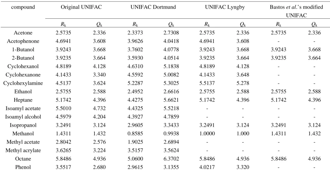
The pure compound data are listed in Table 2; the pure flash points being measured using the Flash Point Analyzer, the Antoine coefficients being sourced from the literature [40-47]. The group volume and surface area parameters, and the UNIFAC group interaction parameters for different UNIFAC-type models were obtained from the literature [18, 21-23, 48-50], with the former two parameters being listed in Table 3, but for some mixtures, group contributions were not available as open literature.

Finally ideal assumption simulation was done for comparison and some non-ideal simulations using NRTL or Wilson equation were used as references to elucidate the predictive capability of the model based on different UNIFAC-type equation, with the binary interaction parameters of NRTL or Wilson equation being adopted from literature [41, 43, 51-60] and listed in Tables 4 and 5.

Evidence of either positive or negative deviation from Raoult’s law was assessed by computing activity coefficient value with the various models cited above. Activity coefficients calculations were done at the flash point temperature.

Activity coefficient behavior helps understanding the flash point behavior. Indeed activity coefficient curves are strongly connected to vapor−liquid equilibrium and azeotropic behavior [61]. And as shown in earlier articles [1-4, 12, 13, 37, 62, 63] and by Eq. (1), flash point is strongly connected to vapor−liquid equilibrium behavior.

4.2 Binary mixtures of flammable solvents

Experimental flash-point data for the sixteen binary mixtures of flammable solvents covering their entire composition ranges are displayed in Figs. 2-7. Octane + heptane, ethanol + 1-butanol and methyl acetate + methyl acrylate are near ideal solutions [1, 27, 43, 51, 52]. The methanol + acetone, ethanol + acetone, methanol + methyl acetate, methanol + methyl acrylate, isoamyl alcohol + isoamyl acetate, octane + 1-butanol, octane + 2-butanol, octane + ethanol, and octane + isopropanol mixtures deviate positively from an ideal solution. The first three mixtures are typical ones of positive deviation from ideality but show no minimum flash point behavior unlike the six others [1, 4, 12, 27]. The four remaining mixtures, cyclohexylamine + cyclohexanol, phenol + acetophenone, phenol + cyclohexanol, and phenol + cyclohexanone, all deviate negatively from ideality, and the latter three exhibit a maximum flash point behavior [29].

4.2.1 Ideal solutions

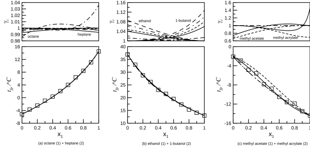
As reported by the literatures [43, 51, 52], the mixtures, octane + heptane, ethanol + 1-butanol and methyl acetate + methyl acrylate, are ideal solutions, thus, the three mixtures were put into the ideal solutions category in this study. Figure 2 compared measured and predicted flash points for the three ideal solutions. Whatever the model used, all predicted results are undistinguishable and in excellent agreement with the experimental data for the octane + heptane and ethanol + 1-butanol (Figure 2(a), 2(b) and Table 6). Indeed, Figure 2 shows that the mean liquid-phase activity coefficient of octane + heptane, defined as the mean value over 101 molar compositions evenly distributed over the entire composition range, computed with the modified UNIFAC Dortmund is 0.9996 over the whole composition range for both compounds, with a minimum value at the other pure component. Unity activity coefficients are a distinctive feature of ideal solutions. For ethanol + 1-butanol, the mean activity coefficient is 1.02 for both compounds, with a maximum value at the other pure components (Fig. 2(b)).

For methyl acetate + methyl acrylate, the mean activity coefficient estimated by the modified UNIFAC Dortmund 93 is 0.89 and 0.86 for methyl acetate and methyl acrylate, respectively, hinting at a non-ideal solution, which is not as the literature reported being an ideal mixture [52]. On the other hand, the original UNIFAC model displays a peculiar behavior, with methyl acrylate activity coefficient reaching a 0.87 minimum value around 70% methyl acetate before ending above unity and methyl acetate activity coefficient showing a maximum 1.04 value. That behavior may be responsible for the shape of the flash point curvature with inflection points. As in Figure 2(a) and 2(b), corresponding to near ideal mixtures, the ideal model predicts a strict decrease of the flash point that disagrees with the experimental data of inflection behavior in Figure 2 (c). On the other hand, the original and the modified Dortmund 93 UNIFAC models correctly predict the inflection points, but the modified UNIFAC-Dortmund 93 is the less accurate (Figure 2(c) and Table 6).

4.2.2 Mixtures with positive deviation from ideality

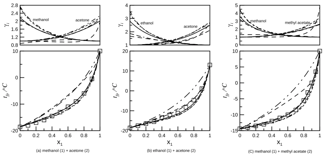
The experimental data indicated that the flash point of a binary solution that reveals a positive deviation from an ideal solution, e.g., methanol + acetone, ethanol + acetone, methanol + methyl acetate, methanol + methyl acrylate, isoamyl alcohol + isoamyl acetate, octane + 1-butanol, octane + 2-butanol, octane + ethanol, or octane + isopropanol, is typically lower than that predicted by the model based upon an ideal solution (Figs. 3-5). Such difference is attributed to the observation that, in accordance to liquid–vapor equilibrium knowledge, the vapor pressure of flammable substances in a solution which demonstrates a positive deviation from an ideal solution is higher than that predicted by Raoult’s law, such that the flash point temperature will be lower than the predictive equivalent based upon an ideal solution. Simulation results assuming an ideal model are indeed very far from the experimental data.

Regarding the non-ideal models used for the simulation, UNIFAC-like models predictions match fairly well the experimental data of mixtures with positive deviation from ideality (Figs. 3-5), although there are still deviations between these predictions and measurements. Among the models, Bastos et al.’s model accuracy is rather chaotic, ranging from good to very poor.

A detailed inspection of Table 6 shows that the NRTL-based predictions have the best predictive capability, with lower deviation of flash point than the other predictions, for methanol + acetone and methanol + methyl acrylate. However, in the cases of ethanol + acetone, methanol + methyl acetate, isoamyl alcohol + isoamyl acetate and octane + ethanol, the predictions based on the original

UNIFAC equation are better than those based on NRTL equation. For octane + 1-butanol and octane + 2-butanol, all UNIFAC-type models based predictions are superior to those of Wilson. The modified UNIFAC-Dortmund 93 predictions are better than those using NRTL equation for isoamyl alcohol + isoamyl acetate and octane + isopropanol, and equivalent for the methanol + acetone and octane + ethanol mixtures. UNIFAC Lyngby predictions are also good, although not as good as the NRTL analogues. However, the prediction performance based on Bastos et al.’s modified UNIFAC model are chaotic, good for ethanol + acetone, octane + 1-butanol and octane + 2-butanol but poor for methanol + acetone, methanol + methyl acetate and octane + ethanol. It may be attributed to the fact that the parameters of Bastos et al.’s modified UNIFAC model were regressed on the data at infinite dilution rather than over the entire composition range. In addition, it is also suspected that there were printing errors in Bastos et al.’s manuscript [23]. Overall, the predictions based on UNIFAC-type models, except for Bastos et al.’s modified one, are comparable to the analogue of NRTL-based.

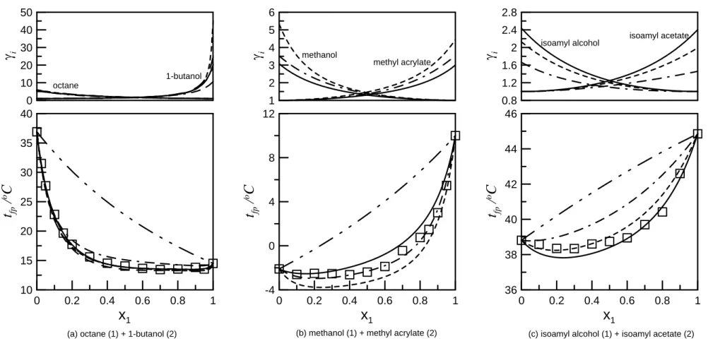
A detailed look at the calculated activity coefficient vs composition curves shows that the larger the positive deviation, the lower the flash point from an ideal solution value (Figs. 3-5): activity coefficients range from 1 to 4.5 for mixtures in Figure 3, and can reach 60 with asymmetrical behavior of each compound in Figure 5 where significant minimum flash point behavior is observed. In Figure 4, minimum flash point behavior is also recorded experimentally but whereas octane + 1-butanol (Figure 4(a)) behaves more like mixtures in Figure 5, methanol + methyl acrylate (Figure 4(b)) and isoamyl alcohol + isoamyl acetate (Figure 4(c)) activity coefficients ranges and symmetrical behavior are like those in Figure 3, although they display a minimum flash point behavior. This could be explained by the closeness of the pure compound flash points in Figure 4(b) and 4(c) (resp. 12.1°C and 6.1°C), unlike the mixtures in Figure 3 where pure compound flash point differences, resp. 28.6°C, 31.6 and 24.4°C in Figure 3(a), 3(b) and 3(c), prevent the occurrence of minimum flash point behavior.

We postulate that the stronger the positive deviation from ideal solution behavior, the more likely the minimum flash point behavior, but that is not likely to occur if the pure compound flash point temperature difference is large. Such a behavior has been acknowledged in azeotrope occurrence [64] and has been used to forecast the occurrence of azeotrope so as to select suitable azeotropic batch distillation processes [65].

The sufficient condition for a binary mixture to form a minimum flash point solution was derived in our previous study as [27]:

(21) 1 , 1 1 1 , 2 > ∞ sat fp T sat P P fp γ (22) 1 , 2 2 2 , 1 ≥ ∞ sat fp T sat P P fp γ

where component 1 is the one with the lower flash point value. For a mixture exhibiting positive deviation from ideality, Eq. (21) is inherently satisfied since the value of sat_fp T sat P P fp 1, 1 / , 2

is greater than unity due to the flash point value of component 2 is greater than that of component 1. In eq. (22), along with the value of

γ

₂∞ relative to components interaction, the sat_fp

T sat P P fp 2, 2 / , 1

value also determine whether Eq. (22) is satisfied or not. The greater the pure component flash point temperature difference is, the less the value of sat_fp

T sat P P fp 2, 2 / , 1

is, and that makes the occurrence of minimum flash point behavior to be difficult.

A review of the literature revealed that only our previously-proposed model [1] and Catoire et al’s model [14, 66] can predict the minimum flash point behavior. In this work, using our model in conjunction with UNIFAC-type models has the advantage of being able to predict such a behavior without necessity of extra experimental binary interaction parameters.

4.2.3 Mixtures with negative deviation from ideality

In contrast to mixtures with positive deviation from ideality, the predicted flash points based on an ideal-solution assumption are typically lower than the corresponding experimental data for mixtures exhibiting a negative deviation from an ideal solution, such as cyclohexylamine + cyclohexanol, phenol + acetophenone, phenol + cyclohexanone, phenol + cyclohexanol (Figs. 6 and 7). This phenomenon is caused by a vapor pressure of such mixtures lower than its value assuming ideal behavior. As a consequence, the flash point will be higher than its ideal-based value.

For all mixtures presented in Figures 6 and 7, NRTL, modified UNIFAC-Dortmund 93 model or the original UNIFAC model correctly predicts the flash point behavior (Table 6), in accordance with the negative deviation of the activity coefficient vs composition curves.

For the systems with phenol (Figure 7), the UNIFAC Lyngby model systematically predicts a positive deviation behavior. Unlike the other UNIFAC models, the UNIFAC Lyngby has no specific “a-OH” hydroxyl group linked to an aromatic ring but a single –OH hydroxyl group contribution that is clearly not adequate for phenol in the light of the flash points prediction. Notice that unlike in

Figure 7(a), UNIFAC Lyngby’s erroneous positive deviation prediction in Figure 7(b) and 7(c) does not translates into a minimum flash point because as in Figures 3(a), 3(b) and 3(c), the difference in the pure compound flash points is large.

Another point worth interest is that in Figure 7(c), the original UNIFAC model predicts by far the strongest negative deviation, reaching 0.13 for cyclohexanol, which explains why the flash point curve has the highest maximum.

In the context of hazard reduction of flammable liquids, the characteristic of mixtures with negative deviation from ideality is essential as it reduces explosion hazard [29]. The application of UNIFAC-type models predictive capacity of the flash-point prediction of such mixtures has not been done before this work but shows great promise. The modified UNIFAC-Dortmund 93 model, with a larger group databank than the original UNIFAC model is particularly accurate.

4.3 Binary aqueous−organic mixtures

The measured flash points of binary aqueous−organic solutions are plotted against the predictive curves in Figure 8. For all mixtures, the predicted values based upon an ideal solution assumption are inaccurate and systematically larger than experimental measurements, in particular above 20% of water. That trend was previously observed for positive deviation binary mixtures of flammable solvents (see Figures 3-5). Indeed, as confirmed by the activity coefficient vs composition curves (Figure 8), such aqueous−organic solutions reveal a positive deviation from that of an ideal solution [2], with such behavior resulting in a reduction of the solution’s flash point from the predicted analogue for an ideal solution. The use of non-ideal models reduces the differences between the predicted and measured values of flash point (Fig. 8 and Table 6).

For all positive deviation mixtures in Figure 8, as the deviation increases (from methanol to propanol), the flash point curve looks more like a chair. For even greater positive deviation there could appear two liquid phases, as observed in liquid−vapor equilibrium behavior. Indeed water mixture with heavier alcohol like 1-butanol, 2-butanol and pentanol exhibits partial miscibility in the flash point curve [63].

For the cases of aqueous solutions of ethanol and isopropanol, the NRTL predictions with the sets of binary-parameter values used for the two aqueous solutions being selected from several ones of our previous study [2] have the best agreement with the experimental data; usually better than the already good predictions based on the UNIFAC-type models, except for Bastos et al.’s model (Table 6). Table 6 demonstrates that for aqueous−methanol solution, the modified UNIFAC Dortmund 93 based predictions is superior to that of NRTL-based, with

the sets of binary-parameter values being also selected from several ones of our previous study [2]; the predictive capability of other UNIFAC-type models are also very good. For the water + n-propanol mixture, NRTL predictions are acceptable but less accurate than those of the UNIFAC-based models, Bastos et al.’s model excepted (Table 6). For that mixture, Bastos et al.’s modified UNIFAC model predicts a wave shape flash point curve, that is typical of mixtures with two liquid phases [4, 37, 62, 63]

Table 6 shows that for water + ethanol, predictions are excellent for xwater ≤ 0.9, with the average flash point deviations being 0.95, 0.88, 0.97 and 0.84 oC when based on the original UNIFAC, the modified UNIFAC-Dortmund 93, the UNIFAC Lyngby and Bastos et al.’s modified UNIFAC model, respectively. For xwater > 0.9, average flash point deviations increase to 5.99, 1.61, 4.00 and 13.67 oC, respectively. This phenomenon of greater deviation in high water composition region was also observed in NRTL-based prediction and in other partially miscible aqueous−organic mixtures [37, 63] and can be explained by the model failure to consider the effect of inert concentration on the lower flammable limit of a mixture [26]. In the estimation of flash point for an aqueous−organic mixture, Eq. (1) uses the Le Chatelier’s rule [67] that assumes that an inert substance such as water has no effect on the lower flammable limit of a mixture. The same trend is also observed for the other binary and ternary aqueous−organic mixtures in this study (Table 6).

Overall, the prediction results of the flash-point prediction model based upon either of the UNIFAC-type models, except for Bastos et al.’s modified UNIFAC one, agree well with the measured flash points corresponding to an aqueous−organic solution, especially for the modified UNIFAC-Dortmund 93 model.

4.4 Ternary mixtures of flammable solvents

Figure 9 compared the predicted flash points, based upon the NRTL and different UNIFAC-type model, with the corresponding measured values for ternary solution of methanol + ethanol + acetone. All non-ideal models perform well, with the NRTL being the best, followed by the original UNIFAC model (Table 6).

Table 6 also demonstrates that the predictions, which assume ideal behavior, deviate from the measurements. The activity coefficients for this solution were indicated by Gmehling et al. [53] to deviate significantly from unity. Thus, ideal solution assumption is not valid for such a non-ideal solution.

The predicted flash points for the other ternary mixture: methanol + methyl acetate + methyl acrylate are compared with the experimental data in Fig. 10. All

non-ideal models predictions display good agreement, although there are slight differences (Table 6). The NRTL equation has the best predictive capability followed by the original UNIFAC based prediction and the modified UNIFAC-Dortmund 93 model predictions.

As was the other ternary mixture, the predictions based upon ideal behavior are not satisfactory (see Table 6) explained by the fact that the activity coefficients for these mixtures deviate notably from unity [52].

4.5 Ternary aqueous−organic mixtures

For ternary aqueous–organic water + methanol + ethanol and water + methanol + isopropanol mixtures (Figures 11 and 12), NRTL and UNIFAC-type models based predictions are entirely consistent with the experimental data although there were slight differences between them (Table 6). Table 6 also shows that in the case of the water + methanol + ethanol mixture, the predictive capability of the modified UNIFAC-Dortmund 93 based was comparable to that of NRTL based. It is emphasized that the NRTL binary interaction parameters used here were regressed on data of ternary solutions, which gave better predictive capability than that with parameters regressed on binary data [3]. For the other water + methanol + isopropanol mixture, any of the three UNIFAC-type models predictions give lower average deviation than with NRTL (Table 6). On the other hand, ideal model based prediction accuracy are markedly lower than that of the non-ideal model predictions, using any of the tested equations to estimate activity coefficients (Table 6).

As with the binary aqueous–organic mixtures, the deviation is larger for xwater > 0.90, likely due to the inability of the Le Chatelier’s rule to incorporate the effect of inert on the lower flammable limit of a mixture [26].

5. Conclusion

We have investigated the ability of activity coefficient for UNIFAC-type models, which do not need any experimental binary interaction parameters, to predict the flash point of flammable and of aqueous–organic binary and ternary mixtures by using the non-ideal flash point model proposed by Liaw and Chiu [3]. Predictions were systematically compared with NRTL or Wilson activity coefficient model based predictions and experimental data taken from literature or first published in this paper.

The combined model is able to represent well the experimental data over the entire flammable composition range of all binary and ternary mixtures, ideal mixtures as well as Raoult’s law negative or positive deviation mixtures. It has also been noticed a relation between the strength of the deviation from Raoult’s law

together with the pure compound flash point difference and the ability of mixture to display a minimum or a maximum flash point behavior: the greater the deviation, the higher the probability for a mixture to exhibit extreme flash point behavior, provided that the pure compound flash point difference is not too large.

For some mixtures, the predictions based on UNIFAC-type models were superior to the NRTL-based or Wilson-based ones. Overall, the model based on the original UNIFAC equation and based on the modified UNIFAC-Dortmund 93 equation are recommended, with a preference for the modified UNIFAC-Dortmund 93 model which provides the most completed database of binary interaction parameters. Besides, as the numbers of groups and interactions available for the modified UNIFAC-Dortmund 93 increase periodically thanks to the UNIFAC consortium, the range of mixtures by application of the modified UNIFAC-Dortmund 93 model in the flash point prediction will increase expectably. Nomenclature

A, B, C =Antoine coefficients Aij = binary parameter (K)

g = binary parameters of the NRTL equation (J/mol) N = number of experimental data

sat i

P = saturated vapor pressure (kPa)

sat fp i

P_, = saturated vapor pressure of component, i, at flash point (kPa) R = gas constant (8.314 J/mol·K)

T = temperature (K)

Ti,fp = flash point temperature of pure component, i (K)

x = liquid-phase composition Greek letters

fp

T

Δ = deviation of flash point αij =NRTL parameter

γ = activity coefficient

λ = binary parameters of Wilson equation (J/mol) Subscripts

exp. = experimental data fp = flash point

i = species i

pred. = predictive value

Acknowledgements

supporting this study financially under grant #NSC 97-2221-E-039-002-MY3. References

[1] H.-J. Liaw, Y.-H. Lee, C.-L. Tang, H.-H. Hsu, J.-H. Liu, J. Loss Prev. Proc. 15 (2002) 429-438.

[2] H.-J. Liaw, Y.-Y. Chiu, J. Hazard. Mater. 101 (2003) 83-106. [3] H.-J. Liaw, Y.-Y. Chiu, J. Hazard. Mater. 137 (2006) 38-46.

[4] H.-J. Liaw, V. Gerbaud, C.-Y. Chiu, J. Chem. Eng. Data 55 (2010) 134-146. [5] H.-J. Liaw, V. Gerbaud, C.-C. Chen, C.-M. Shu, J. Hazard. Mater. 177 (2010)

1093-1101.

[6] D.A. Crowl, J.F. Louvar, Chemical Process Safety: Fundamentals with Applications, 2nd ed., Prentice Hall PTR, New Jersey, 2002.

[7] CCPS/AIChE, Guidelines for Engineering Design for Process Safety, 1st ed., American Institute of Chemical Engineers, New York, 1993.

[8] Regulations, Regulation (EC) No. 1272/2008 of the European Parliament and of the Council, on Classification, Labeling and Packaging of Substances and Mixtures, Amending and Repealing Directives 67/548/EEC and 1999/45/EC, and amending Regulation (EC) No. 1907/2006, Official J. Eur. Union, 2008, L353. [9] W.A. Affens, G.W. McLaren, J. Chem. Eng. Data 17 (1972) 482-488.

[10] D. White, C.L. Beyler, C. Fulper, J. Leonard, Fire Safety J. 28 (1997) 1-31. [11] R.W. Garland, M.O. Malcolm, Process Saf. Prog. 21 (2002) 254-260. [12] H.-J. Liaw, C.-L. Tang, J.-S. Lai, Combust. Flame 138 (2004) 308-319. [13] H.-J. Liaw, T.-A. Wang, J. Hazard. Mater. 141 (2007) 193-201.

[14] L. Catoire, S. Paulmier, V. Naudet, J. Phys. Chem. Ref. Data 35 (2006) 9-14. [15] J. Gmehling, P. Rasmussen, Ind. Eng. Chem. Fundam. 21 (1982) 186-188. [16] S.-J. Lee, D.-M Ha, Korean J. Chem. Eng. 20 (2003) 799-802.

[17] A. Fredenslund, R.L. Jones, J.M. Prausnitz, AIChE J. 21 (1975) 1086.

[18] A. Fredenslund, J. Gmehling, M.L. Michelsen, P. Rasmussen, J.M. Prausnitz, Ind. Eng. Chem. Process Des Dev. 16 (1977) 450-462.

[19] M. Vidal, W.J. Rogers, M.S. Mannan, Process Saf. Environ. Prot. 84 (2006) 1-9. [20] U. Weidlich, J. Gmehling, Ind. Eng. Chem. Res. 26 (1987) 1372-1381.

[21] J. Gmehling, J. Li, M. Schiller, Ind. Eng. Chem. Res. 32 (1993) 178-193.

[22] B.L. Larsen, P. Rasmussen, A. Fredenslund, Ind. Eng. Chem. Res. 26 (1987) 2274-2286.

[23] J.C. Bastos, M.E. Soares, A.G. Medina, Ind. Eng. Chem. Res. 27 (1988) 1269-1277.

[24] T. Magnussen, P. Rasmussen, A. Fredenslund, Ind. Eng. Chem. Process Des Dev. 20 (1981) 331-339.

[25] H. Hooper, S. Michel., J.M. Prausnitz, Ind. Eng. Chem. Res. 27 (1988) 2182-2187.

[26] M.G. Zabetakis, Flammability Characteristics of Combustible Gases and Vapors, U.S. Dept of the Interior, Bureau of Mines, Washington, 1965.

[27] H.-J. Liaw, T.-P. Lee, J.-S. Tsai, W.-H. Hsiao, M.-H. Chen, T.-T. Hsu, J. Loss Prevent. Proc. 16 (2003) 173-186.

[28] H.-J. Liaw, C.-T. Chen, C.-C. Cheng, Y.-T. Yang, J. Loss Prevent. Proc. 21 (2008) 82-100.

[29] H.-J. Liaw, S.-C. Lin, J. Hazard. Mater. 140 (2007) 155-164.

[30] D.-M. Ha, S. Lee, M.-H. Back, Korean J. Chem. Eng. 24 (2007) 551-555.

[31] Y. Guo, F. Yang, Y. Xing, D. Li, W. Fang, R. Lin, Fluid Phase Equilibr. 276 (2009) 127-132.

[32] D. Li, W. Fang, Y. Xing, Y. Guo, R. Lin, J. Hazard. Mater. 161 (2009) 1193-1201.

[33] Y. Xing, D. Shao, W. Fang, Y. Guo, R. Lin, Fluid Phase Equilibr. 284 (2009) 14-18.

[34] M. Noorollahy, A. Zarringhalam Moghadam, A. Ameri Ghasrodashti, Chem. Eng. Res. Des. 88 (2010) 81-86.

[35] ASTM D 56, Standard Test Method for Flash Point by Tag Closed Tester, American Society for Testing and Materials, West Conshohocken, PA, 1999. [36] The UNIFAC Consortium, http://unifac.ddbst.de/ (accessed 2010).

[37] H.-J. Liaw, V. Gerbaud, H.-T. Wu, J. Chem. Eng. Data (in press) (2010) doi:10.1021/je100163q.

[38] Oxford University, The Physical and Theoretical Chemistry Laboratory,

http://msds.chem.ox.ac.uk/IS/isoamyl_alcohol.html (accessed 2010).

[39] Dow Chemical Company, http://www.dow.com/PublishedLiterature/dh_015f/0901b8038015f0df.pdf?filepat

h=custproc/pdfs/noreg/114-00072.pdf&fromPage=GetDoc (accessed 2010). [40] B.E. Poling, J.M. Prausnitz, J.P. O’Connell, The Properties of Gases and Liquids,

5th ed., McGraw-Hill, New York, 2001.

[41] J. Gmehling, U. Onken, W. Arlt, Vapor-Liquid Equilibrium Data Collection, Vol. 1, Part 2b, DECHEMA, Frankfurt, Germany, 1978.

[42] T. Boublik, V. Fried, E. Hala, The Vapor Pressures of Pure Substances, 2nd ed., Elsevier, Amsterdam, 1984.

[43] J. Wisniak, R. Reich, H. Segura, Fluid Phase Equilibr. 154 (1999) 213-222. [44] J. Gmehling, U. Onken, P. Grenzheuser, Vapor-Liquid Equilibrium Data

Collection, Part 5, DECHEMA, Frankfurt, Germany, 1987.

323-327.

[46] J.A. Riddick, W.B. Bunger, T.K. Sakano, Organic Solvents, 4th ed., Wiley, New York, 1986.

[47] R.C. Reid, J.M. Prausnitz, T.K. Sherwood, The Properties of Gases and Liquids, third ed., McGraw-Hill, New York, 1977.

[48] S. Skjold-Jørgensen, B. Kolbe, J. Gmehling, P. Rasmussen, Ind. Eng. Chem. Process Des. Dev. 18 (1979) 714-722.

[49] J. Gmehling, P. Rasmussen, A. Fredenslund, Ind. Eng. Chem. Process Des. Dev. 21 (1982) 118-127.

[50] E.A. Macedo, U. Weidlich, J. Gmehling, P. Rasmussen, Ind. Eng. Chem. Process Des. Dev. 22 (1983) 676-678.

[51] H. Kosuge, K. Iwakabe, Fluid Phase Equilibr. 233 (2005) 47-55. [52] C.H. Tu, Y.S. Wu, T.L. Liu, Fluid Phase Equilibr. 135 (1997) 97-108.

[53] J. Gmehling, U. Onken, Vapor-Liquid Equilibrium Data Collection, Vol. 1, Part 2a., DECHEMA, Frankfurt, Germany, 1977.

[54] M.C. Iliuta, F.C. Thyrion, Fluid Phase Equilibr. 103 (1995) 257-284. [55] L.S. Lee, R.G. Lin, Fluid Phase Equilibr. 165 (1999) 261-278.

[56] T. Hiaki, A. Taniguchi, T. Tsuji, M. Hongo, K. Kojima, J. Chem. Eng. Data 41 (1996) 1087-1090.

[57] A. Arce, A. Blanco, A. Soto, I. Vidal, Fluid Phase Equilibr. 128 (1997) 261-270. [58] A. Arce, J. Martinez-Ageitos, J. Mendoza, A. Soto, Fluid Phase Equilibr. 141

(1997)207-220.

[59] R.A. Dawe, D.M.T. Newsham, S.B. Ng, J. Chem. Eng. Data 18 (1973) 44-49. [60] J. Gmehling, U. Onken, W. Arlt, Vapor-Liquid Equilibrium Data Collection, Part

1a. DECHEMA, Frankfurt, Germany, 1981.

[61] I. Shulgin, K. Fischer, O. Noll, and J. Gmehling, Ind. Eng. Chem. Res. 40 (2001) 2742–2747.

[62] H.-J. Liaw, W.-H. Lu, V. Gerbaud, C.-C. Chen, J. Hazard. Mater. 153 (2008) 1165-1175.

[63] H.-J. Liaw, C.-T. Chen, V. Gerbaud, Chem. Eng. Sci. 63 (2008) 4543-4554. [64] L.Berg, Chem. Eng. Prog. 65 (1969) 52-57

[65] V. Gerbaud, X. Joulia, I. Rodriguez-Donis, O. Baudouin, O. Rosemain, A. Vacher, P. Castelain, Chem. Eng. Proc. 45 (2006) 672-683,

[66] L. Catoire, S. Paulmier, V. Naudet, Process Saf. Prog. 25 (2006) 33-39. [67] H. Le Chatelier, Ann. Mines 19 (1891) 388-395.

FIGURE LEGENDS

Figure 1. The basic system configuration of the Tag close cup tester.

Figure 2. Comparison of predicted flash point and experimental data for ideal solutions. , experimental data; , original UNIFAC; ,UNIFAC Dortmund 93; , UNIFAC Lyngby; , Bastos et al.’s modified UNIFAC; , NRTL;

, ideal solution.

Figure 3. Comparison of predicted flash point and experimental data for mixtures with positive deviation from ideal solutions. , experimental data; , original UNIFAC; ,UNIFAC Dortmund 93;

, UNIFAC Lyngby; , Bastos et al.’s modified

UNIFAC; , NRTL; , ideal solution.

Figure 4. Comparison of predicted flash point and experimental data for mixtures just forming minimum flash point solution. , experimental data; , original UNIFAC; ,UNIFAC Dortmund 93;

, UNIFAC Lyngby; , Bastos et al.’s modified UNIFAC; , NRTL/Wilson; , ideal solution. Figure 5. Comparison of predicted flash point and experimental data for minimum

flash point solutions. , experimental data; , original

UNIFAC; ,UNIFAC Dortmund 93; , UNIFAC

Lyngby; , Bastos et al.’s modified UNIFAC; , NRTL/Wilson; , ideal solution.

Figure 6. Comparison of predicted flash point and experimental data for cyclohexylamine (1) + cyclohexanol (2). , experimental data;

, original UNIFAC; ,UNIFAC Dortmund 93;

, UNIFAC Lyngby; , NRTL; ,

ideal solution.

Figure. 7. Comparison of predicted flash point and experimental data for maximum flash point solutions. , experimental data; , original

UNIFAC; ,UNIFAC Dortmund 93; , UNIFAC

Lyngby; , NRTL; , ideal solution.

Figure 8. Comparison of predicted flash point and experimental data for some aqueous-organic solutions. , experimental data; ,

original UNIFAC; ,UNIFAC Dortmund 93; ,

UNIFAC Lyngby; , Bastos et al.’s modified UNIFAC; , NRTL; , ideal solution.

(1) + ethanol (2) + acetone (3). , experimental data;

blue / , original UNIQUAC;

red / , UNIFAC Dortmund 93;

green / , UNIFAC Lyngby;

yellow / , NRTL.

Figure 10. Comparison of predicted flash point with experimental data for methanol (1) + methyl acetate (2) + methyl acrylate (3). , experimental data;

blue / , original UNIQUAC;

red / , UNIFAC Dortmund 93;

yellow / , NRTL.

Figure 11. Comparison of predicted flash point with experimental data for water (1) + methanol (2) + ethanol (3). , experimental data; blue

/ , original UNIQUAC; red / ,

UNIFAC Dortmund 93; green / , UNIFAC

Lyngby; yellow / , NRTL.

Figure 12. Comparison of predicted flash point with experimental data for water (1) + methanol (2) + isopropanol (3). , experimental data;

blue / , original UNIQUAC;

red / , UNIFAC Dortmund 93;

green / , UNIFAC Lyngby; yellow

Table 1 Measured flash point for binary mixtures Tfp/oC x1 Octane (1)+ heptane (2) Methyl acetate (1) + methyl acrylate (2) Octane (1) + 1-butanol (2) Methanol (1) + methyl acrylate (2) Isoamyl alcohol (1) + isoamyl acetate (2) Octane (1) + ethanol (2) Octane (1) + 2-butanol (2) Octane (1) + isopropanol (2) 0.0 -5.2 -2.1 36.9 a -2.1 38.8 a 13.0 22.0 a 12.9 0.01 - - - 11.7 b - - 0.02 - - - 9.5 20.5 b 11.7 b 0.025 - - 31.5 - - - 0.03 - - - 9.1 b 19.0 b - 0.05 - - 27.7 - - 7.5 17.9 a 9.8 a 0.1 -3.7 a -2.9 a 22.8 -2.6 38.6 a 5.6 15.2 8.0 a 0.12 - - - 14.6 - 0.15 - - 19.7 - - - 0.2 -2.5 a -4.9 a 17.8 a -2.5 a 38.4 a 4.8 a 13.0 a 6.6 0.3 -1.0 a -5.6 a 15.6 a -2.5 a 38.3 a 4.8 a 11.9 a 6.4 0.35 - - - 6.5 a 0.4 0.3 a -7.8 a 14.5 a -2.6 38.6 a 4.8 a 11.1 a 6.3 a 0.5 2.1 a -8.8 a 14.1 a -2.4 a 38.7 a 4.7 a 11.0 a 6.4 a 0.6 4.0 a -10.5 13.7 b -1.9 39.0 a 4.8 a 10.7 a 6.7 a 0.7 6.4 a -11.6 13.5 a -0.4 a 39.7 a 5.0 10.8 a 6.5

0.8 8.4 -11.9 a 13.6 a 0.8 a 40.4 a 5.2 a 10.8 a 7.1 a 0.85 - - - 1.5 a - - - 7.7 b 0.9 11.1 a -13.5 13.8 a 3.0 42.6 a 5.2 a 11.2 a 8.1 0.93 - - - 8.4 a 0.95 - - 13.5 b 5.5 - 5.9 a 11.0 b 8.5 b 0.96 - - - 6.5 - - 0.97 - - - 7.6 b - 9.1 a 0.98 - - - 8.8 b 12.1 b 9.5 a 0.99 - - - 10.3 b 12.8 b 10.9 b 0.992 - - - 12.1 b - - 0.994 - - - 12.6 b - - 0.995 - - - 13.0 b - 11.9 b 1.0 14.5 a -14.4 14.5 a 10.0 44.9 a 14.5 a 14.5 a 14.5 b

new data, first published here a

Table 2 Antoine coefficients and experimental flash point for studied solution components Antoine coefficients Substance A B C Reference Tfp,exp/oC e Acetone d 4.21840 1197.010 -45.090 [40] -18.6 ± 0.9 Acetophenone c 7.45474 1950.500 -49.118 [41] 83.5 ± 1.7 1-Butanol a 6.54068 1335.028 -96.496 [42] 36.9 ± 2.8 2-Butanol a 6.32690 1157.363 -104.830 [42] 22.0 ± 2.4 Cyclohexanol c 8.35237 2258.560 -21.376 [41] 67.2 ± 3.5 Cyclohexanone c 7.47050 1832.200 -28.800 [41] 47.0 ± 2.0 Cyclohexylamine c 6.68954 1229.418 -84.198 [41] 28.6 ± 1.0 Ethanol a 7.24222 1595.811 -46.702 [42] 13.0 ± 0.6 Heptane a 6.02023 1263.909 -56.718 [43] -5.2 ± 0.5 Isoamyl acetate a 6.31940 1473.280 -52.202 [44] 38.8 ± 1.1 Isoamyl alcohol d 4.07851 1128.190 -126.680 [40] 44.9 ± 2.2 Isopropanol a 7.56634 1366.142 -75.030 [45] 12.9 ± 0.8 Methanol a 7.20519 1581.993 -33.289 [46] 10.0 ± 0.8 Methyl acetate d 4.18621 1156.430 -53.460 [40] -14.4 ± 0.6 Methyl acrylate b 16.10880 2788.430 -59.150 [47] -2.1 ± 0.8 Octane a 6.04394 1351.938 -64.030 [45] 14.5 ± 1.4 Phenol d 4.26960 1523.420 -97.750 [40] 81.3 ± 4.6 n-Propanol d 4.99991 1512.940 -67.343 [40] 21.5 ± 2.3 a log(P/kPa)=A-B/[(T/K)+C] b ln(P/mmHg)=A-B/[(T/K)+C] c log(P/mmHg)=A-B/[(T/K)+C] d log(P/bar)=A-B/[(T/K)+C] e

Table 3 group volumes and group surface areas used in the UNIFAC-type models

Original UNIFAC UNIFAC Dortmund UNIFAC Lyngby Bastos et al.’s modified

UNIFAC compound Rk Qk Rk Qk Rk Qk Rk Qk Acetone 2.5735 2.336 2.3373 2.7308 2.5735 2.336 2.5735 2.336 Acetophenone 4.6941 3.608 3.9626 4.0418 4.6941 3.608 - - 1-Butanol 3.9243 3.668 3.7602 4.0778 3.9243 3.668 3.9243 3.668 2-Butanol 3.9235 3.664 3.5930 4.0514 3.9235 3.664 3.9235 3.664 Cyclohexanol 4.8189 4.128 4.6310 5.1838 4.8189 4.128 - - Cyclohexanone 4.1433 3.340 4.5592 5.0082 4.1433 3.648 - - Cyclohexylamine 4.5137 3.624 5.2287 5.3025 5.5137 5.278 - - Ethanol 2.5755 2.588 2.4952 2.6616 2.5755 2.588 2.5755 2.588 Heptane 5.1742 4.396 4.4275 5.6621 5.1742 4.396 5.1742 4.396 Isoamyl acetate 5.5010 4.732 4.4325 5.5218 - - - - Isoamyl alcohol 4.5979 4.204 4.3927 4.7859 - - - - Isopropanol 3.2491 3.124 2.9605 3.3433 3.2491 3.124 3.2491 3.124 Methanol 1.4311 1.432 0.8585 0.9938 1.0000 1.000 1.4311 1.432 Methyl acetate 2.8042 2.576 1.9025 2.6894 - - - - Methyl acrylate 3.6265 3.224 3.5157 3.5624 - - - - Octane 5.8486 4.936 5.0600 6.3702 5.8486 4.936 5.8486 4.936 Phenol 3.5517 2.680 2.9615 3.1355 4.0217 3.320 - -

n-Propanol 3.2499 3.128 3.1277 3.3697 3.2499 3.128 3.2499 3.128 water 0.9200 1.400 1.7334 2.4561 0.9200 1.400 0.9200 1.400

Table 4 VLE parameters of the NRTL or Wilson equation for the studied binary solutions a

Mixtures A12 A21 α12 Reference

Octane (1) + heptane (2) 226.8700 -179.6800 0.3000 [43] Ethanol (1) + 1-butanol (2) 38.0723 -32.9414 0.3038 [51] Methyl acetate (1)+ methyl

acrylate (2)

-3.8691 2.3936 0.2979 [52] Ethanol (1) + acetone (2) 230.4142 -16.1714 0.3025 [53]

Methanol (1) + acetone (2) 140.0460 78.3170 0.4700 [54] Methanol (1) + methyl acetate

(2)

86.2370 224.9900 0.2710 [52]

Methanol (1) + methyl acrylate (2)

214.3700 164.8900 0.2484 [52]

Isoamyl acetate (1) + isoamyl alcohol (2) 173.0100 -13.9690 0.4700 [55] Octane (1) + 1-butanol (2) 114.3300 667.1000 - [56] Octane (1) + 2-butanol (2) 111.2700 515.4200 - [56] Octane (1) + ethanol (2) 604.9700 651.9100 0.4700 [45] Octane (1) + isopropanol (2) 478.3500 450.2100 0.4694 [41] Cyclohexylamine (1) + cyclohexanol (2) -29.4840 -149.4000 0.3033 [41] Phenol (1) + acetophenone (2) 140.3000 -500.5100 0.3051 [41] Phenol (1) + cyclohexanol (2) -199.7600 -233.0800 0.3080 [41] Phenol (1) + cyclohexanone (2) 140.3000 -500.5100 0.3051 [41] Water (1) + methanol (2) 487.7900 -214.1500 0.1000 [57] Water (1) + ethanol (2) 523.8400 3.1700 0.3000 [58] Water (1) + n-propanol (2) 865.4100 77.3300 0.3772 [59] Water (1) + isopropanol (2) 797.9600 -22.9800 0.2882 [60] a Wilson: Aij= (λij-λii)/R; NRTL: Aij= (gij-gjj)/R

Table 5 VLE parameters of the NRTL equation for the studied ternary solutions Parameters a Methanol (1) + methyl acetate (2) + methyl acrylate (3) [52] Methanol (1) + ethanol (2) + acetone (3) [53] Water (1) + methanol (2) + ethanol (3) [60] Water (1) + methanol (2) + isopropanol (3) [60] A12 101.1200 -257.9900 311.4430 595.5180 A21 227.6500 361.3500 -96.0690 -189.0620 A13 174.9600 39.6100 536.6630 885.2480 A31 215.1800 194.4300 -26.9570 -4.4760 A23 -57.6850 244.9800 111.4220 262.8850 A32 83.7550 -61.7900 -109.6060 -211.3360 α12 0.2710 0.3000 0.3020 0.3190 α13 0.2484 0.2960 0.2920 0.2910 α23 0.2979 0.3080 0.3100 0.3040 a Aij= (gij-gjj)/R

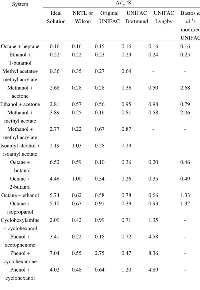
Table 6 Deviation between calculated and experimental flash points, a, for the studied mixtures, comparing models

fp T Δ fp T Δ /K System Ideal Solution NRTL or Wilson Original UNIFAC UNIFAC Dortmund UNIFAC Lyngby Bastos et al.’s modified UNIFAC Octane + heptane 0.16 0.16 0.15 0.16 0.16 0.16 Ethanol + 1-butamol 0.22 0.22 0.23 0.23 0.24 0.25 Methyl acetate+ methyl acrylate 0.36 0.35 0.27 0.64 - - Methanol + acetone 2.68 0.28 0.28 0.36 0.50 2.68 Ethanol + acetone 2.81 0.57 0.56 0.95 0.98 0.79 Methanol + methyl acetate 3.89 0.25 0.16 0.81 0.58 2.06 Methanol + methyl acrylate 2.77 0.22 0.67 0.87 - - Isoamyl alcohol + isoamyl acetate 2.19 1.03 0.28 0.29 - - Octane + 1-butanol 6.52 0.59 0.10 0.36 0.20 0.46 Octane + 2-butanol 4.46 1.00 0.34 0.26 0.35 0.49 Octane + ethanol 5.74 0.62 0.58 0.78 0.66 1.33 Octane + isopropanol 5.10 0.67 0.91 0.39 0.93 1.32 Cyclohexylamine + cyclohexanol 2.09 0.42 0.99 0.71 1.35 - Phenol + acetophenone 3.41 0.22 0.18 0.72 4.58 - Phenol + cyclohexanone 7.04 0.55 2.75 0.47 8.36 - Phenol + cyclohexanol 4.02 0.48 0.64 1.20 4.89 -

Water + methanol 8.87 b 17.56 c 3.65 d 1.00 b 1.31 c 0.81 d 1.10 b 1.97 c 0.58 d 0.89 b 0.85 c 0.91 d 1.21 b 2.00 c 0.74 d 1.81 b 3.29 c 0.92 d Water + ethanol 17.35 b 34.57 c 7.97 d 0.45 b 0.72 c 0.31 d 2.71 b 5.94 c 0.95 d 1.13 b 1.61 c 0.88 d 2.04 b 4.00 c 0.97 d 5.37 b 13.67 c 0.84 d Water + n-propanol 26.54 b 53.31 c 7.80 d 2.51 b 4.96 c 0.79 d 2.30 b 4.23 c 0.95 d 1.40 b 2.63 c 0.54 d 2.06 b 3.91 c 0.77 d 4.66 b 8.46 c 2.00 d Water + isopropanol 22.36 b 46.59 c 7.82 d 1.31 b 2.27 c 0.74 d 3.91 b 8.40 c 1.21 d 1.60 b 3.28 c 0.60 d 2.27 b 4.26 c 1.07 d 6.22 b 12.95 c 2.19 d Methanol + ethanol + acetone 3.15 0.33 0.69 1.18 1.31 - Methanol + methyl acetate + methyl acrylate 3.20 0.27 0.40 0.70 - - Water + methanol + ethanol 9.81 b 22.77 c 2.84 d 0.64 b 0.99 c 0.46 d 1.96 b 3.38 c 1.20 d 0.85 b 1.525 c 0.49 d 1.38 b 2.91 c 0.56 d - Water + methanol + isopropanol 10.16 b 29.20 c 3.13 d 2.11 b 6.52 c 0.49 d 1.96 b 4.10 c 1.17 d 1.58 b 3.42 c 0.90 d 1.28 b 2.69 c 0.77 d - a

deviation of flash point: T T T N

N pred fp fp fp =

∑

,exp.− , . / Δ b _ΔT

fp over the entire flammable range

c _ΔT

fp for mole fraction of water greater than 0.9

d _ΔT

0 0.2 0.4 0.6 0.8 1

x

₁ -8 -4 0 4 8 12 16

t

fp

/

o

C

0 0.2 0.4 0.6 0.8 1

x

₁ -16 -12 -8 -4 0

t

fp

/

o

C

(a) octane (1) + heptane (2) (c) methyl acetate (1) + methyl acrylate (2)

0 0.2 0.4 0.6 0.8 1

x

₁ 10 15 20 25 30 35 40

t

fp

/

o

C

(b) ethanol (1) + 1-butanol (2) 0.98 0.99 1 1.01 1.02 1.03 1.04

γ

i octane heptane 1 1.04 1.08 1.12 1.16

γ

i _{ethanol 1-butanol} 0.6 0.8 1 1.2 1.4 1.6

γ

i

methyl acetate methyl acrylate

Figure 2. Comparison of predicted flash point and experimental data for ideal solutions. , experimental data; , original

UNIFAC; ,UNIFAC Dortmund 93; , UNIFAC Lyngby; , Bastos et al.’s modified UNIFAC;

0 0.2 0.4 0.6 0.8 1

x

₁ -20 -10 0 10

t

fp

/

o

C

(a) methanol (1) + acetone (2)

0 0.2 0.4 0.6 0.8 1

x

₁ -20 -10 0 10 20

t

fp

/

o

C

(b) ethanol (1) + acetone (2) 0 0.2 0.4 0.6 0.8 1

x

₁ -15 -10 -5 0 5 10

t

fp

/

o

C

(C) methanol (1) + methyl acetate (2)

0.8 1.2 1.6 2 2.4 2.8

γ

i methanol acetone 1 2 3 4

γ

i ethanol acetone 0 1 2 3 4 5

γ

i methanol methyl acetate

Figure 3. Comparison of predicted flash point and experimental data for mixtures with positive deviation from ideal solutions. ,

experimental data; , original UNIFAC; ,UNIFAC Dortmund 93; , UNIFAC Lyngby;

0 0.2 0.4 0.6 0.8 1

x

₁ 10 15 20 25 30 35 40

t

fp

/

o

C

0 0.2 0.4 0.6 0.8 1

x

₁ -4 0 4 8 12

t

fp

/

o

C

(a) octane (1) + 1-butanol (2) (b) methanol (1) + methyl acrylate (2)

0 0.2 0.4 0.6 0.8 1

x

₁ 36 38 40 42 44 46

t

fp

/

o

C

(c) isoamyl alcohol (1) + isoamyl acetate (2)

0 10 20 30 40 50

γ

i octane 1-butanol 1 2 3 4 5 6

γ

i _methanol methyl acrylate 0.8 1.2 1.6 2 2.4 2.8

γ

i

isoamyl alcohol isoamyl acetate

Figure 4. Comparison of predicted flash point and experimental data for mixtures just forming minimum flash point solution. ,

experimental data; , original UNIFAC; ,UNIFAC Dortmund 93; , UNIFAC Lyngby;

0 0.2 0.4 0.6 0.8 1

x

₁ 0 4 8 12 16 fp o

t

/

C

0 0.2 0.4 0.6 0.8 1

x

₁ 8 12 16 20 24

t

fp

/

o

C

(a) octane (1) + ethanol (2) _{(b) octane (1) + 2-butanol (2)}

(c) octane (1) + isopropanol (2) 0 0.2 0.4 0.6 0.8 1

x

₁ 4 6 8 10 12 14 16

t

fp

/

o

C

0 10 20 30 40

γ

i octane isopropanol 0 10 20 30 40

γ

i octane 2-butanol 0 20 40 60 80

γ

i octane ethanol

Figure 5. Comparison of predicted flash point and experimental data for minimum flash point solutions. , experimental data;

, original UNIFAC; ,UNIFAC Dortmund 93; , UNIFAC Lyngby; , Bastos et al.’s

f

0

0.2

0.4

0.6

0.8

1

x

₁

20

30

40

50

60

70

la

s

h

p

o

in

t (

o

C)

Figure 6. Comparison of predicted flash point and experimental data for cyclohexylamine (1) + cyclohexanol (2). , experimental data;

, original UNIFAC; ,UNIFAC Dortmund 93;

, UNIFAC Lyngby; , NRTL; , ideal

solution.

0.2

0.4

0.6

0.8

1

cyclohexylamine cyclohexanol

0 0.2 0.4 0.6 0.8 1

x

₁ 80 82 84 86 88 90 92

t

fp

/

o

C

0 0.2 0.4 0.6 0.8 1

x

₁ 40 50 60 70 80 90

t

fp

/

o

C

(a) phenol (1) + acetophenone (2) (b) phenol (1) + cyclohexanone (2)

0 0.2 0.4 0.6 0.8 1

x

₁ 64 68 72 76 80 84 88

t

fp

/

o

C

(c) phenol (1) + cyclohexanol (2) 0 0.4 0.8 1.2 1.6

γ

i phenol acetophenone 0 0.4 0.8 1.2 1.6

γ

i phenol cyclohexanol 0 0.4 0.8 1.2 1.6

γ

i phenol cyclohexanone

Figure 7. Comparison of predicted flash point and experimental data for maximum flash point solutions. , experimental data;

, original UNIFAC; ,UNIFAC Dortmund 93; , UNIFAC Lyngby; , NRTL;

0 0.2 0.4 0.6 0.8 1

x

₁ 0 20 40 60 80

t

fp

/

o

C

(a) water (1) + methanol (2)

0 0.2 0.4 0.6 0.8 1

x

₁ 0 20 40 60 80 (b) water (1) + ethanol (2) 0 0.2 0.4 0.6 0.8 1

x

₁ 20 40 60 80 (c) water (1) + propanol (2) 0 0.2 0.4 0.6 0.8 1

x

₁ 0 20 40 60 80 (d) water (1) + isopropanol (2) 0.8 1.2 1.6 2 2.4 2.8

γ

2 0 2 4 6 8 10 0 5 10 15 20 25 0 5 10 15 20 25

Figure 8. Comparison of predicted flash point and experimental data for some aqueous-organic solutions. , experimental data;

, original UNIFAC; ,UNIFAC Dortmund 93; , UNIFAC Lyngby; , Bastos et al.’s

-25 -20 -15 -10 -5 0 5 10 15 0.0 0.2 0.4 0.6 0.8 1.0 0.0 0.2 0.4 0.6 0.8

T

fp

/

o

C

x

1

x

₂ 0 0.2 0.4 0.6 0.8 1

x

₂ -20 -10 0 10 20

T

fp

/

o

C

x1=0 x1=0.1 x1=0.2 x1=0.3 x1=0.4 x1=0.5 x1=0.6 x1=0.7 x1=0.8 x1=0.9 x1=1.0

(a) three dimensional plot (b) two dimensional plot

Figure 9. Comparison of predicted flash point with experimental data for methanol (1) + ethanol (2) + acetone (3). (complete data sets available

from the authors upon request) , experimental data; blue / , original UNIQUAC; red / ,

-20 -15 -10 -5 0 5 10 15 0.0 0.2 0.4 0.6 0.8 1.0 0.0 0.2 0.4 0.6 0.8

T

fp

/

o

C

x

1

x

₃ 0 0.2 0.4

_x

0.6 0.8 1 1 -15 -10 -5 0 5 10

T

fp

/

o

C

x₂=0 x₂=0.1 x₂=0.2 x₂=0.3 x₂=0.4 x₂=0.5 x₂=0.6 x₂=0.7 x₂=0.8 x₂=0.9 x₂=1

(a) three dimensional plot (b) two dimensional plot

Figure 10. Comparison of predicted flash point with experimental data for methanol (1) + methyl acetate (2) + methyl acrylate (3). (complete data sets available from the authors upon request) , experimental data; blue / , original UNIQUAC;

0 20 40 60 80 100 0.0 0.2 0.4 0.6 0.8 1.0 0.0 0.2 0.4 0.6 0.8

T

fp

/

o

C

x

1

x

₂ 0 0.2 0.4 0.6 0.8 1

x

₂ 0 20 40 60 80 100

T

fp

/

o

C

x1=0 x1=0.1 x1=0.2 x1=0.3 x1=0.4 x1=0.5 x1=0.6 x1=0.7 x1=0.8 x1=0.9 x1=0.95 x1=0.97 x1=0.98

(a) three dimensional plot (b) two dimensional plot

Figure 11. Comparison of predicted flash point with experimental data for water (1) + methanol (2) + ethanol (3). (complete data sets a ailable v from the authors upon request) , experimental data; blue / , original UNIQUAC;

red / , UNIFAC Dortmund 93; green / , UNIFAC Lyngby; yellow

0 20 40 60 80 100 0.0 0.2 0.4 0.6 0.8 1.0 0.0 0.2 0.4 0.6 0.8 1.0

T

fp

/

o

C

x

1

x

₂ 0 0.2 0.4 0.6 0.8 1

x

₂ 0 20 40 60 80

T

fp

/

o

C

x₁=0 x₁=0.1 x₁=0.2 x₁=0.3 x₁=0.4 x₁=0.5 x₁=0.6 x₁=0.7 x₁=0.8 x₁=0.91 x₁=0.95 x₁=0.97 x₁=0.98

(a) three dimensional plot

(b) two dimensional plot

Figure 12. Comparison of predicted flash point with experimental data for water (1) + methanol (2) + isopropanol (3). (complete data sets available from the authors upon request) , experimental data; blue / , original UNIQUAC;

red / , UNIFAC Dortmund 93; green / , UNIFAC Lyngby; yellow