Study of Integration Schemes Suited for the Long-Term Extrapolation

Open Archive TOULOUSE Archive Ouverte (OATAO)

This is an author-deposited version published in : http://oatao.univ-toulouse.fr/

Eprints ID : 13809

To cite this version : Anton, Julie and Trilles, Sébastien and Mercier,

Pierre Study of Integration Schemes Suited for the Long-Term Extrapolation. (2011) In: 22nd International Symposium on Space Flight Dynamics, 28 February 2011 - 4 March 2011 (Sao José dos Campos, Brazil)

Any correspondance concerning this service should be sent to the repository administrator: staff-oatao@listes-diff.inp-toulouse.fr

STUDY OF INTEGRATION SCHEMES SUITED FOR THE LONG-TERM EXTRAPOLATION

Julie ANTON (1), Sébastien TRILLES (2), Pierre MERCIER(3)

(1) THALES C4I, Defense and Security / ISAE-ENSICA, 3 avenue de l’Europe, bât. 2D, 31400 Toulouse (France), julie.anton@thalesgroup.com

(2) THALES C4I, Defense and Security, 3 avenue de l’Europe, bât. 2D, 31400 Toulouse (France), sebatien.trilles@thalesgroup.com

(3) THALES C4I, Defense and Security, 3 avenue de l’Europe, bât. 2D, 31400 Toulouse (France), pierre.mercier@thalesgroup.com

Abstract: This paper is focused on the integration methods for the orbit extrapolation on the long term

time. This issue is of importance when it comes to choosing the graveyard orbit during the orbit design process for a space mission. In this paper, classical and geometric integration schemes will be discussed and compared on LEO (Low Earth Orbit) cases. We will give a particular interest to the variational scheme, in the last chapter, since this geometric integrator has the property of preserving the geometry of the problem like symplectic schemes but, contrary to symplectic integrators, it can be also used in case of non conservative dynamics.

Keywords: extrapolation, long-term, symplectic, variational, end-of-life. 1. Introduction

Major current concerns, such as the tracking of space debris or spacecraft end-of-life disposal, have increased the need for efficient long term extrapolation study tools : for instance, deorbitation maneuver, for future LEO missions, will have to be computed such that the spacecraft reenters the Earth atmosphere within 25 years. Usually an uncontrolled reentry is chosen because it is the cheapest solution. All the difficulty is to find the optimal and thus the less costly orbit in terms of propellant that is to say the nearest from the initial one from which the satellite will effectively reenter the Earth atmosphere naturally within 25 years. During the preliminary phase of orbit design, this optimal end-of-life orbit can be found through an iterative process which explains the importance of using an efficient extrapolator tool in terms of accuracy and, above all, speed.

This article is focused on the extrapolation methods despite the fact that the result i.e. the derived ephemerid depends also on the physical model. Thus, to be more accurate and more precise, one can also work on the way to define the physical model.

In this paper, we will take a particular interest in the problem of determining rapidly and accurately the disposal orbit of a satellite from a Low Earth Orbit. First we will see a classical method of integration which seems well suited for extrapolation on the long term then we will introduce the symplectic integrators and explain why their property of conserving the volumes is interesting for the long term. Finally we will see the interest of using variational integrators rather than symplectic integrators for orbital mechanics problems.

2. Collocation method

2.1. Introduction and justification

Our work on the numerical integration field brought us to explore in more details a new highly-effective method developed by Yu.F.Kolyuka and O.K. Margorin [1]. In particular, their paper is focused on problems of space dynamics which “require to fulfill the calculation of space body orbits

with the highest possible accuracy within long-term time, and at the same time to provide the high speed of computation”. This current issue includes, among others, the tracking of space debris and the

spacecraft end-of-life disposal problems discussed earlier in the introduction. Moreover, this new high effective method was designed, among other criteria, to “achieve any given accuracy, including the

highest possible one for typical computers, and to keep this accuracy within a long term period of integration,” and to “provide high speed of computations”. All of these reasons have motivated a

detailed study of the new method developed by Yu.F.Kolyuka and O.K. Margorin that we will explain next.

In the following we will see that the integration scheme developed by Yu.F.Kolyuka and O.K. Margorin is actually a modified collocation method.

2.2. Method

We consider a first order of differential equation system of the form :

(1)

The general idea is to approximate the solution of the differential equation (Eq. 1) over an interval , with and h the step size of the numerical integration method, by a polynomial. This polynomial is such that it satisfies the differential equation (Eq. 1) at particular points called collocation points within the interval and its value at agrees with an approximated given value of the solution. All of the difficulty is to correctly choose these collocation points in order to get the best approximation of the physical solution. The number and location of collocation points determine different methods. The higher order of accuracy is reached by using the so called Gauss Legendre distribution of the nodes at the roots of a shifted Legendre polynomial [2].

Let be the n distinct collocation points (usually between 0 and 1). The collocation polynomial is a polynomial of degree n which satisfies :

for

(2)

The numerical solution of the collocation method is given by .

According to the theorem of Guillou and Soulé (1969), the collocation method is equivalent to the n-stage Runge Kutta method with the following coefficients :

and where is the Lagrange interpolation polynomial

.

By introducing the coefficient k defined as followed : and by using the Lagrange interpolation formula to get the continuous polynomial : , we can write the collocation polynomial as following:

for

The collocation methods (Eq. 3) can be seen as implicit Runge Kutta methods. Because it is an implicit method, at each step, the collocation polynomial has to be determined by a prediction-correction process.

2.3. Kolyuka Margorin scheme

The method specifically developed by Yu.F. Kolyuka and O.K. Margorin [1] is a slightly modified collocation method. This method has some particularities compared to the classical scheme. It has two main specificities : its step size is variable and the order of the method can change during the integration to keep the desired accuracy.

This method can be used either for a first or a second order differential equation system. Here we will focus our study only on first order differential systems.

As we have seen before, one of the important aspects of the collocation scheme concerns the choice of the collocation points since they define different methods. Here, they have been chosen to work with symmetrical distributions between -1 and 1 that include the points -1, 0 and 1. The points are chosen such that they are very close to the Tchebychev roots.

The control of the step size allows to keep a given accuracy during the integration. Indeed, if the step size is too large compared to the optimal one, which can be computed only at the end of the step, then there are two solutions in order to keep the desired accuracy : either the step size can be reduced to the optimal one and the step computed again or the distribution of collocation points can be increased by two points in order to increase the order of the method. Between the two solutions, the latter is the less costly in terms of calculation time since it avoids decreasing the step size. Therefore, Yu.F. Kolyuka and O.K. Margorin propose to use an embedded set of collocation points.

2.4. Tests

To test this integration scheme, we will use an operational software which has been developed for internal uses and which is adapted to the long term extrapolation.

For the LEO cases, this software takes into account, in terms of perturbations, the luni-solar attraction, the gravitational perturbation (terms J2, J3, J4 and J2²) and the atmospheric drag. Since we are interested in the long term behavior, we only take into account the long-term and very long-term variations. We are only interested in the mean motion of the spacecraft. The differential equations system is the Gauss system. This software is written in JAVA language.

We tested on this software the following integrators : Runge Kutta 4, Runge Kutta 6, Collocation method with the 4th order Lobatto III distribution, the Kolyuka Margorin integrator with a fixed step size and with the distribution . We present here the results of two tests realized among the 20 tests :

– test case 15 : the initial parameters are , , , , , , , , NLRMSISE-00 as atmospheric model, a constant solar activity of 140 sfu and a magnetic activity of .

– test case 19 : the initial parameters are , , ,

, , , , , NLRMSISE-00 as atmospheric model, a constant solar activity of 140 sfu and a magnetic activity of .

Figure 1. Test case 15 and Test case 19: Spacecraft end-of-life and computation time obtained with different integrators.

The results (Fig. 1) show that, due to the smooth physical model, all kind of integrators can be used. They all present approximately the same results in terms of precision. The scaling factor is the problem's dynamics. Therefore, the more suited integrator here is the fastest one i.e. the Runge Kutta 4. As it seems that no further improvements can be obtained by proceeding this way, it has been decided to tackle the problem by a different approach that will be discussed in the next section.

3. Lagrange d'Alembert approach 3.1. Symplectic integrators

Our researches on numerical integration methods for long-term issues lead us, in the end, to focus our study on the symplectic integrators. This kind of integrators results from a geometric approach of the problem which differs from the traditional one. The quality of being symplectic means that the integration scheme will well preserve the geometry as well as most of the invariants (e.g. energy) of the problem which are very interesting properties when it comes to determining the orbit of a spacecraft or a celestial body on the long term, with a given precision. Because of their properties of conservation, for a same precision and a same step size, symplectic integrators are usually more efficient than non symplectic integrators. As a result, the step size can be increased with a reasonable energy loss (a symplectic integrator preserves a modified energy close to the real one, the energy loss is controlled over the integration) and without any degradation of the numerical results. [3]

leads us to focus our study on such integrators. 3.1.1. Method and philosophy

The theory is based on the principle of least action which is widely used in classical mechanics to determine the path and states of a physical system. The classical equations of motion of a system can be derived from this principle. Classical mechanics postulates that the trajectory actually followed by a physical system is the one for which the action is minimized/optimized where the action is given (Hamilton's principle) by:

where L is the Lagrangian where – , with T the kinetic energy and V the potential energy. From this principle, we can derive the Euler-Lagrange equations applied for only conservative systems:

(4)

Using Legendre transformations to derive the Hamiltonian formulation (positions and momenta dependence) from the Lagrangian one (positions and velocities dependence), we can rewrite these ODEs as a 1 order differential system called Hamilton’s equations :

and (5)

where H is the Hamiltonian defined by p is the kinetic momentum,

q is the position,

This formulation is very simple and then more suited for a numerical resolution of the differential equations system. This formulation is directly connected to a particular geometry: the symplectic geometry which is the natural framework of a large number of mechanical problems. The symplectic group is the one which preserves the symplectic structure and then the Hamiltonian flow.

3.1.2. Motivation

The major interest of the symplectic structure is to associate unequivocally, to an energy function H, a vector field which describes the physical motion of the system. The way the function H ( on its domain) determines the vector field is directly bounded to the symplectic structure of the phase space . This vector field is given by the symplectic gradient dH of H which leads to the Hamiltonian equations through the definition of the symplectic structure.

Moreover, the vector field

is obviously of null divergence therefore, according to Liouville’s theorem, all Hamiltonian systems preserve the volumes of the space phase.

vector field therefore the equations which are propagated through the integration are still solution of the Hamiltonian problem hence the volumes are preserved (Liouville’s theorem).

Thus, the geometrical structure of the problem is preserved through the integration process which introduces an additional constraint compared to “classical” integrators. This additional constraint will lead to a better control of the physical trajectory which underlines the interest of symplectic integrators. 3.1.3. Examples and limitation

We consider the mathematical pendulum (mass , massless rod of length , gravitational acceleration ). This system has one degree of freedom and its Hamiltonian has the following form : (this Hamiltonian is separable).

So the Hamilton's equations are :

and (6) Figure 2. The pendulum The Hamiltonian flow of these equations (Eq. 6) is symplectic and

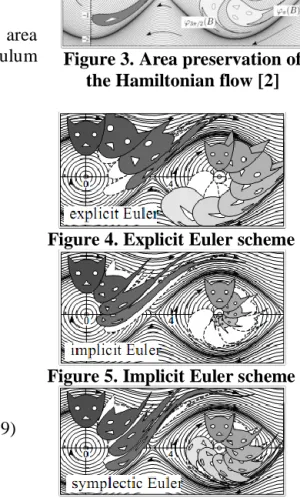
then area preserving. The figure 3 as shown in the opposite illustrates the area preservation of the exact flow for the system in the phase space [2].

The following figures (Fig. 4, 5, 6 and 7) show the area preservation of three numerical methods for the pendulum equations in the phase space.

Figure 3. Area preservation of the Hamiltonian flow [2]

Explicit Euler scheme

(7)

Figure 4. Explicit Euler scheme

Implicit Euler scheme

(8)

Figure 5. Implicit Euler scheme

Symplectic Euler scheme

(9)

Störmer-Verlet scheme

(10)

NB : explicit scheme because H is separable

Figure 7. Störmer-Verlet scheme

We can notice that both explicit and implicit Euler schemes present wrong behavior patterns. For the first one, the motion of the pendulum amplifies and the pendulum wins energy over time, the trajectories diverge, the motion is unstable. For the second one, the motion is thus stable but the pendulum loses energy over time and the trajectories collapse in one point. As to the symplectic Euler scheme, we can notice that the physical behavior is much better, the energy is best-preserved. The Euler symplectic integrator is qualitatively better that the classical ones i.e. the explicit one and the implicit one. The Störmer Verlet scheme which is also a symplectic integrator is even better.

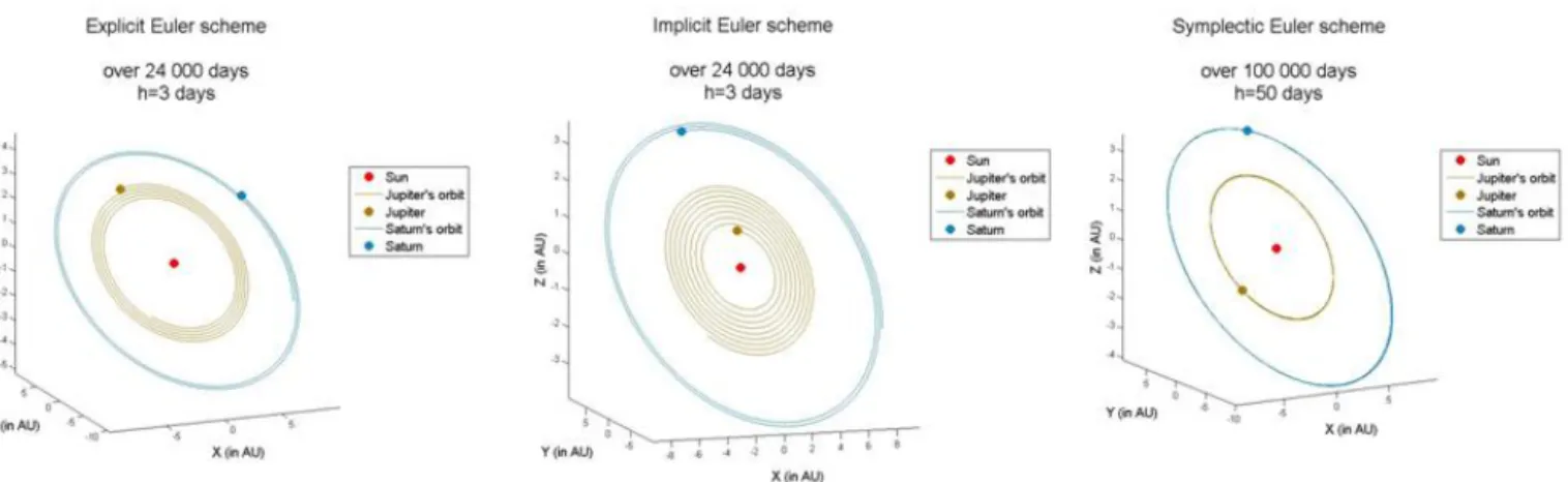
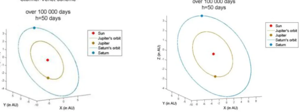
Now, we consider the N body problem which is an Hamiltonian system. The Hamiltonian has the following form :

We simulate this problem with Matlab. To that end, we take into account only three bodies : the Sun, Jupiter and Saturn. We apply to this system the explicit and the implicit Euler methods both with a step size of 3 days and over a period of 24 000 days. We apply also to this system two symplectic methods : the symplectic Euler method and the Störmer-Verlet method both with a step size of 50 days and over a period of 100 000 days. The initial position are taken from p. 14 of the reference [2].

Figure 8. N body problem with different integration schemes Table 1. Computation time for the different integration schemes Computation time Explicit Euler Implicit Euler Symplectic

Euler Störmer-Verlet Lobatto IIIA-IIIB (3 stages) h=3days period=24000days 0.85 s 1.58 s 1.81 s 3.14 s 12.70 s h=50days period=100000days 0.22 s 0.49 s 0.46 s 0.83 s 7,46 s

(The results have been obtained with Matlab on a computer with the processor : Intel Core 2 Duo CPU T6500 @ 2.10 GHz)

Considering the same integration scheme (Fig. 8), we can notice that the behavior of the planets is similar to the behavior of the cat head shaped volume that moves on the phase portrait (Fig. 4, 5, 6 and 7). With the explicit Euler method, Saturn and Jupiter spiral outwards, the planets show an increasing energy. With the implicit Euler method, Jupiter and then Saturn fall towards the Sun and if we increase the simulation period, first Jupiter and then Saturn will be ejected. On the contrary, the symplectic Euler scheme, the Störmer-Verlet scheme and the Lobatto IIIA-IIIB scheme (a symplectic collocation method) all show correct behavior. We can perform an integration over a larger period and we can also use a larger step size (in order to decrease the computation time) without any deterioration of the physical behavior. If we compare the final positions of Jupiter and Saturn obtained with the symplectic integrators, we observe that the uncertainty of the propagator is entirely reported on the tangential component. A symplectic propagator ensures the stability of the radial component and thus the physical coherence of the problem. Thus, the quality of a symplectic integrator depends on the tangential error. Symplectic integrators are therefore very interesting when it comes to determining the orbit of a spacecraft or a celestial body on the long term, without any degradation of the information. They combine a very good radial precision with a short computation time (Tab. 1) which makes them powerful integrators. However, they only concern Hamiltonian systems i.e. conservative ones which is physically most often not the case. Therefore, another approach is needed. It will be the subject of next part.

3.2. Variational approach 3.2.1. Method and philosophy

As mentioned before, the Hamiltonian approach of the problem supposes that there are no dissipative forces acting on the spacecraft which is usually not the case. Here we will present a different approach that will circumvent these limitations. Dissipative forces such as the solar radiation pressure or the

atmospheric drag have usually to be included in the problem's dynamics. To bypass this problem, it is possible to consider a temporal Hamiltonian for example. The other way is to use another approach to solve the problem : the variational one which leads to variational integrators. In the following, we will see that variational integration schemes combine the great advantages of being as powerful as symplectic integrators with the handling of non conservative forces.

Here, the general idea is also based on the least action principle. The starting point of the theory is the Lagrange d'Alembert principle which differs from the least action principle by the fact that non conservative forces are also taken into account.

(11)

where is an infinitesimal perturbation of the path at each point, this displacement is of course null for the endpoints which are fixed.

In order to derive from this principle the variational integration scheme, we will now discretize the Lagrange d'Alembert principle and not the equations of motion as it is usually done for the other integrators (with the Taylor series for the Euler scheme for instance). Indeed, variational integrators will result from discrete Lagrangian mechanics and more precisely from the discrete Euler Lagrange equation associated with a discrete Lagrangian.

For this purpose, instead of a continuous path with , we will consider a discrete path with and , being the approximated value of . Then, we define the discrete Lagrangian on the time interval , where is the time step interval, described as following :

The right hand side integral can be approximated, for example, by a one-point quadrature formula i.e. by the time step length multiplied by the value of the Lagrangian evaluated somewhere between the two points and .As for the velocity, it is simply approximated by the slope between and

:

where . Then the least action principle can be written under its discrete form :

(12)

The infinitesimal variation of the discrete action sum Sd is given by:

where is the partial derivative of L with respect to the first slot and is the partial derivative of L with respect to the second slot.

Since the endpoints are fixed, we can rewrite the previous expression (Eq. 13) as following :

(14)

The continuous forcing can be approximated by :

where and are the left and right discrete forces.

The discrete Lagrange d'Alembert principle can thus be written as:

(15) From the equation 15, because and _{are fixed points so} , we can define the forced discrete Euler-Lagrange equations :

(16) 3.2.2. Scheme

This discrete Lagrange d'Alembert equation defines the following discrete evolution map : . However, for a mechanical system, it is more convenient to work with a position and a velocity (or momentum) rather than two positions. The transformation which allows us to switch from a two-position-variable set to a position-momentum set without any information loss is called the Legendre transformation FL.

Let Q be the configuration space, in our case . We consider TQ the tangent space of Q which can be seen as a phase space with position and velocity as local coordinates (Lagrangian frormalism). So we see the Lagrangian as a smooth map

We use the cotangent space, , which can be seen as a phase space with position and momentum as local coordinates (Hamiltonian formalism).

As before we have a smooth map

The two couple of variables and are bounded by the Legendre transformation seen as a fiber derivative map :

The Legendre transformation is defined by :

In the local chart of TQ where U is an open set around a point and E a space vector such that ,

FL can be viewed as the derivative of the Lagrangian L over the point u at vector e along the fiber E in the direction a :

i.e. is a linear form on the tangent space E over q.

Just as the standard Legendre transformation maps the Lagrangian phase space TQ to the Hamiltonian phase space , we can define discrete Legendre transformations . These discrete transformations map the discrete phase space to [5].

which can be written as:

(17) If we add dissipative forces to the system, then we have to use the forced discrete Legendre transformations written as following [5]:

(18)

Let us consider a Lagrangian of the standard form :

The discrete form of the Lagrangian has already been defined and an approximation by a one-point quadrature formula of the integral form of L over the interval , where is the time step interval, has been proposed. Of course, it is not the only way to approximate this integral (one can use the midpoint rule or the trapezoidal rule... to get a discrete Lagrangian [5]). In our discussion, we will consider the following discrete Lagrangian :

where . Therefore : . In the same way, we define the non conservative discrete forces:

For a forced system, the variational algorithm is deduced from the Legendre transformation (Eq. 18) and the discrete Lagrange d'Alembert equations (Eq. 16):

(19)

This leads to the following variational algorithm :

(20)

One kind of variational scheme is the Newmark algorithm which will be used afterwards[4]:

(21)

With _{the evaluated acceleration.} , otherwise the scheme is not variational

4. Tests

We consider a spacecraft on a low orbit around the Earth. Its orbit has the following characteristics: , , , , ,

In this context, we take into account the following perturbations:

- oblatness of the Earth with the coefficients and , - the lunisolar attraction designed as proposed by Méeus in [6],

- the atmospheric drag with a density simply defined according to King-Hele’s law.

With Matlab, we will propagate the equations of motion (in position/velocity) of this spacecraft around the Earth subjected to the set of perturbations previously described, over a period of 5 years with a step size of 1 min. To this purpose, we will use several integration schemes, among others the Newmark scheme (with and ), and we will compare the results between the different integrators in terms of precision and speed. To discuss the obtained precision, we will take for reference the results given by Cowell, an integrator known for its precision.

Without any perturbations the results for the difference between the experimental and the theoretical semi major axis are the following:

Figure 9. Cowell without perturbations Figure 10. RK6 without perturbations

Figure 11. Newmark without perturbations

Without any perturbation, the semi major axis should be unchanged. However we can notice that it is not the case whatever the chosen integrator. For the Cowell (Fig.9), the semi major axis decreases and, for the Runge Kutta 6 (Fig.10), it increases over time therefore the energy varies. The error is about 13 m at the end of the integration. As for the Cowell, the error is only about 2mm which can be neglected. The Cowell is taken as a reference here because of its high precision. As for the Newmark (Fig.11), the semi major axis oscillates over time but remains constant in average. Hence it is less precise than the Cowell or the Runge Kutta 6, but its behavior respects the physics of the problem. What should prove to be more interesting is its behavior with perturbations (see below).

0 200 400 600 800 1000 1200 1400 1600 1800 2000 -4 -3 -2 -1 0 1 2x 10 -3 time (days) d if fe re n c e w it h t h e t h e o re ti c a l s e m i m a jo r a x is ( m ) Cowell 0 200 400 600 800 1000 1200 1400 1600 1800 2000 0 2 4 6 8 10 12 14 time (days) d if fe re n c e w it h t h e t h e o re ti c a l s e m i m a jo r a x is ( m ) RK6 0 200 400 600 800 1000 1200 1400 1600 1800 2000 0 10 20 30 40 50 60 70 80 90 time (days) d if fe re n c e w it h t h e t h e o re ti c a l s e m i m a jo r a x is ( m ) Newmark (1/4,1/2)

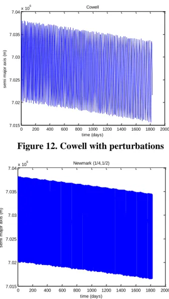
With the perturbations the results for the semi major axis are the following:

Figure 12. Cowell with perturbations Figure 13. RK6 with perturbations (computation time: 2 h 20 min 11 s)

Figure 14. Newmark with perturbations (computation time: 41 min 15s)

When we add the perturbations, the semi major axis slightly decreases over time because of the drag which is a non conservative force. The amplitude (about 17 km) is mainly due to the J2 effect. We can notice that the behavior of both Newmark (Fig.14) and Runge Kutta 6 (Fig. 13) integrators is correct, they both respect the physics of the problem. The final mean semi major axis for the Newmark integrator is equal to 7025.503 km. As for the Runge Kutta 6, its final mean semi major axis is equal to 7024.568 m. Given that the reference i.e. Cowell gives a final semi major axis at 7024.679 m, the Runge Kutta 6 is the closest one from the reference. However, in terms of computation time, Newmark integrator is 3 times faster than Runge Kutta and with a precision of the same order of magnitude.

In terms of computation time, given that the Cowell (written in a compiled language) runs in 20 min 58s for this case, the Newmark algorithm should be much faster if one uses a compiled language. One could therefore imagine that the time step of our second order Newmark scheme could be sufficiently diminished in order to challenge the tenth order Cowell integrator both in accuracy and calculation time.

(The results have been obtained with Matlab on a computer with the processor : Intel Core 2 Duo CPU T6500 @ 2.10 GHz)

5. Conclusion

As a conclusion, geometric integrators and in particular variational integrators, such as Newmark, are suited for the extrapolation on the long term because they are simple and thus efficient in terms of

0 200 400 600 800 1000 1200 1400 1600 1800 2000 7.015 7.02 7.025 7.03 7.035 7.04x 10 6 time (days) s e m i m a jo r a x is ( m ) Cowell 0 200 400 600 800 1000 1200 1400 1600 1800 2000 7.015 7.02 7.025 7.03 7.035 7.04x 10 6 time (days) s e m i m a jo r a x is ( m )

Evolution of the semi major axis RK6 h=60 s over a period of 5 years

0 200 400 600 800 1000 1200 1400 1600 1800 2000 7.015 7.02 7.025 7.03 7.035 7.04x 10 6 time (days) s e m i m a jo r a x is ( m ) Newmark (1/4,1/2)

computation time and they also respect the physics of the problem on the long term. For problems with dissipation, which is usually the case for orbital mechanics problems, variational integrators have shown the required behavior. This paper has therefore highlighted the fact that other schemes exists that may be as precise as the Cowell integrator if the time step is sufficiently small as well as faster. Work is in progress at Thales to set up a new variational scheme that will improve the precision without any consequent rise of the calculation time.

Acknowledgments : The authors are most grateful to Thierry Authié for his help concerning the last validation part.

6. References

[1] Kolyuka, Yu.F. and Margorin, O.K., “The New High-Effective Method for Numerical Integration of Space Dynamics Differential Equations”, 1995.

[2] Hairer, E., Lubich, C., Wanner, G., “Geometric Numerical Integration : Structure-Preserving Algorithms for Ordinary Differential Equations”, Second Edition, Springer.

[3] Vilmart, G., “Etude d'intégrateurs géométriques pour des équations différentielles”, 2008.

[4] Kane, C., Marsden, J.E., Ortiz, M. and West, M., “Variational Integrators and Newmark Algorithm for Conservative and Dissipative Mechanical Systems”, 1999.

[5] West, M., “Variational Integrators”, 2004. [6] Méeus, J., “Astronomical Algorithms”, 1999.