Pépite | Développement de la méthode SPH (smoothed particle hydrodynamics) pour simuler les caractéristiques de base de la dynamique des méandres

Texte intégral

(1)Thèse de Dwinanti Rika Marthanty, Lille 1, 2016. N° … UNIVERSITÉ DES SCIENCES ET TECHNOLOGIES DE LILLE 1 Ecole Doctorale Science Pour l’Ingénieur Université Lille Nord-de-France THÈSE Présentée et soutenue en vue de l’obtention du grade de Docteur Spécialité Génie Civil en Hydrodynamique et Mécanique des Fluides Numérique Par Dwinanti Rika MARTHANTY. Développement de la méthode SPH (smoothed particle hydrodynamics) pour simuler les caractéristiques de base de la dynamique des méandres Soutenue le 26 avril 2016 devant la Commission d’Examen composée de : Pr. Isam SHAHROUR. Prof. Dedi Priadi Pr. Erick CARLIER Dr-Ing. Dwita Sutjiningsih Herr Soeryantono, PhD Pr. Hassan SMAOUI Prof. Iwan Kridasantausa Hadihardaja. © 2016 Tous droits réservés.. Laboratoire Génie Civil et géoEnvironnement, Université Lille 1, France Faculty of Engineering, Universitas Indonesia, Indonesia École Polytech Lille, Université Lille 1, France Departemen Teknik Sipil, Universitas Indonesia, Indonesia Departemen Teknik Sipil, Universitas Indonesia, Indonesia Laboratoire Roberval, Université Technologie de Compiègne, France Departemen Teknik Sipil, Institut Teknologi Bandung, Indonesia. Directeur de laboratoire Dean Directeur de thèse Promotor Co-promotor Rapporteur Reader. lilliad.univ-lille.fr.

(2) Thèse de Dwinanti Rika Marthanty, Lille 1, 2016. UNIVERSITAS INDONESIA. DEVELOPING SMOOTHED PARTICLE HYDRODYNAMICS METHOD TO MODEL BASIC CHARACTERISTICS OF MEANDERING DYNAMICS. DISSERTATION a dissertation submitted to the Doctoral Program in Civil Engineering in conformity with the requirements for the Degree of Doctor in the fields of Hydrodynamics and Computational Fluid Dynamics. Dwinanti Rika Marthanty NPM.1006751640 INE.0CPZRL05TL5. Double Degree Program Indonesia - France Departemen Teknik Sipil, Universitas Indonesia, Indonesia Laboratoire Génie Civil et géo-Environnement, Université Lille 1, France. June 2016. i Universitas Indonesia – Université de Lille 1 © 2016 Tous droits réservés.. lilliad.univ-lille.fr.

(3) Thèse de Dwinanti Rika Marthanty, Lille 1, 2016. STATEMENT OF ORIGINALITY AND AUTHENTICITY. I hereby declare that this dissertation is my own work, and for all references cited, I have stated all correctly.. Name: Dwinanti Rika Marthanty NPM: 1006751640. Signature: ……............................. Date: …….……………. ii Universitas Indonesia – Université de Lille 1.

(4) Thèse de Dwinanti Rika Marthanty, Lille 1, 2016. © 2016 Tous droits réservés.. lilliad.univ-lille.fr.

(5) Thèse de Dwinanti Rika Marthanty, Lille 1, 2016. HALAMAN PERNYATAAN PERSETUJUAN PUBLIKASI TUGAS AKHIR UNTUK KEPENTINGAN AKADEMIS. Sebagai sivitas akademik Universitas Indonesia, saya yang bertanda tangan di bawah ini: Nama : Dwinanti Rika Marthanty NPM : 1006751640 Program Studi : Teknik Sipil Departemen : Teknik Sipil Fakultas : Teknik Jenis karya : Disertasi demi pengembangan ilmu pengetahuan, menyetujui untuk memberikan kepada Universitas Indonesia Hak Bebas Royalti Noneksklusif (Non-exclusive Royalty Free Right) atas karya ilmiah saya yang berjudul : DEVELOPING SMOOTHED PARTICLE HYDRODYNAMICS METHOD TO MODEL BASIC CHARACTERISTICS OF MEANDERING DYNAMICS beserta perangkat yang ada (jika diperlukan). Dengan Hak Bebas Royalti Noneksklusif ini Universitas Indonesia berhak menyimpan, mengalihmedia/formatkan, mengelola dalam bentuk pangkalan data (database), merawat, dan memublikasikan tugas akhir saya selama tetap mencantumkan nama saya sebagai penulis/pencipta dan sebagai pemilik Hak Cipta. Demikian pernyataan ini saya buat dengan sebenarnya.. Dibuat di : Depok, Jawa Barat, Indonesia Pada tanggal : ……………………. Yang menyatakan. (Dwinanti Rika Marthanty). iv Universitas Indonesia – Université de Lille 1.

(6) Thèse de Dwinanti Rika Marthanty, Lille 1, 2016. ABSTRACT Name: Dwinanti Rika Marthanty Study Program: Civil Engineering Title: Developing Smoothed Particle Hydrodynamics Method to Model Basic Characteristics of Meandering Dynamics Meanders occur even without sediment transport, it is caused by a large-scale turbulence (da Silva, 2006). Meandering channels research in general is separated, but still correlated, into two approaches: geomorphologic and fluid dynamics, where 3D flow modeling receives more attention for its ability to simulate helicoidal motion even though it is high in computational efforts and limited to simple geometry (Camporeal, et al., 2007). One developed model with a finite element method for three-dimensional flow is called Resource Modelling Associates (RMA), to model; density stratified flow (RMA10), and water quality in estuaries and streams (RMA-11) (King, 2013). Smoothed particle hydrodynamics (SPH) is one most noticeable meshfree method and now become very popular, particularly for free surface flows, it is a robust and powerful method for describing deforming media (Gomez-Gesteira, et al., 2010). SPH is a very promising method to answer 3D flow modeling in meander dynamics. Objective of this research that helical flow patterns from flow simulation with 3D nearly incompressible flow SPH method is comparable to flow simulation with 3D stratified flow finite element method. Approaches in this research is divided into two big parts; (1) modeling meander dynamics with RMA to determine its basic characteristics, and (2) development smoothed particle hydrodynamics (SPH) method to simulate helical flow in a curved channel. The finite element model using in this study, RMA has shown its capability to simulate the meander key characteristics and are agreed with experiments of Hasegawa (1983), and Xu and Bai (2013). These results are used as a reference in developing a method to model meander dynamics. SPH procedures are developed from 3D fluid flow model, collision handling between water particles, and curved channel boundary conditions. The very basic characteristic in meander dynamics is helical flow. With SPH simulation, helical flow is initiated by adding up viscous flow and vorticity at initial conditions. Formation of helical flow is generated at downstream hemispheres part of the curved channel. Helical flow pattern from SPH model can be compared with helical flow patterns from RMA model. The helical flow pattern is consistent with the patterns from very recently experiment investigation by Wang and Liu (2015), and theoretical sketch of secondary flows in a curved channel by Wu (2008). Thus, SPH method is able to develop helical flow as a result of curvature, agreed with Camporeal et al. (2007), and even without sediment transport, agreed with da Silva (2006) and Yalin (1993). Our contribution with this research is developing SPH method for modeling helical flow in a curved channel with the aim of simulating meandering dynamics. This is all along with advancement of SPH in Hydraulics where four grand challenges in SPH applications, according to SPHERIC community (Violeau & Rogers, 2015), are convergence, numerical stability, boundary conditions, and adaptivity. This research participates to the two of SPH challenges; boundary conditions and adaptivity. We used simple geometries based on Snell’s law to represent basic particle responses to channel walls. We adapted SPH for nearly incompressible flow as a basic hydraulics phenomenon in a curved channel that is note bene an incompressible flow. Keywords: smoothed particle hydrodynamics, RMA, helical flow, 3D fluid flow simulation, curved channel, meandering. v Universitas Indonesia – Université de Lille 1 © 2016 Tous droits réservés.. lilliad.univ-lille.fr.

(7) Thèse de Dwinanti Rika Marthanty, Lille 1, 2016. RÉSUMÉ DE THÉSE Méandres se produire même sans le transport des sédiments, elle est causée par une turbulence à grande échelle (da Silva, 2006). La recherche de méandre des chaînes en général est séparé, mais toujours corrélée, en deux approches : la dynamique géomorphologiques et fluide, où la modélisation des flux 3D reçoivent plus d'attention pour sa capacité à simuler le mouvement hélicoïdal, même si elle est élevée dans les efforts de calcul et limitée à une géométrie simple (Camporeal, et al, 2007). Un modèle développé avec un finis méthodes d'éléments pour l'écoulement en trois dimensions est appelé Resource Modelling Associates (RMA), pour modéliser ; flux de densité stratifié (RMA-10), et la qualité de l'eau dans les estuaires et les ruisseaux (RMA-11) (King, 2013). Smoothed particle hydrodynamics (SPH) est une méthode libre de maille la plus perceptible et devenu très populaire, en particulier pour les flux de surface libre, il est une méthode robuste et puissant pour décrire les médias déformation (Gomez-Gesteira, et al, 2010). SPH est une méthode très prometteuse pour répondre à la modélisation des flux 3D dans le dynamique méandre. Objectif de cette recherche est modèles d'écoulement hélicoïdaux de simulation d'écoulement avec 3D méthode SPH d'écoulement presque incompressible est comparable à écouler simulation avec écoulement stratifié 3D méthode des éléments finis. Approches dans cette recherche est divisé en deux grandes parties ; (1) modélisation du dynamique méandre avec RMA afin de déterminer ses caractéristiques de base, et (2) développement de la méthode de SPH pour simuler l'écoulement hélicoïdal dans un canal. Modèle éléments finis utilisé dans cette étude, RMA a montré sa capacité à simuler les caractéristiques clés de méandres et sont convenus avec les expériences de Hasegawa (1983), et Xu et Bai (2013). Ces résultats sont utilisés comme référence pour développer le modèle du dynamique méandre. Procédures de SPH sont élaborées à partir du modèle d'écoulement du fluide 3D, gestion des collisions entre les particules de l'eau, et des conditions aux limites de canal courbes. La caractéristique fondamentale dans le dynamique méandre est écoulement hélicoïdal. Avec simulation de SPH, écoulement hélicoïdal est initiée par l'addition des flux de tourbillon et visqueux aux conditions initiales. Formation d'écoulement hélicoïdal est généré en hémisphères partie aval du canal courbé. Motif d'écoulement hélicoïdal à partir du modèle SPH peut être comparé avec des modèles de flux hélicoïdaux de modèle RMA. Le modèle d'écoulement hélicoïdal est compatible avec les modèles de l'investigation très récente de l'expérience par Wang et Liu (2015), et l’esquisse théorique de flux secondaires dans un canal courbe par Wu (2008). Ainsi, SPH est capable pour développer écoulement hélicoïdal du fait de la courbure, d'accord avec Camporeal et al. (2007), et même sans le transport des sédiments, convenu avec da Silva (2006) et Yalin (1993). Notre contribution en présente recherche est le développement de la méthode SPH pour la modélisation de l'écoulement hélicoïdal dans un canal courbé dans le but de simuler le dynamique méandre. Ceci est tout le long avec l'avancement de SPH en hydraulique où quatre grands défis dans les applications de SPH, selon la communauté SPHERIC (Violeau et Rogers, 2015), sont la convergence, la stabilité numérique, la condition limite, et l'adaptabilité. Cette recherche participe aux deux défis de SPH ; la condition limite et l’adaptabilité. Nous avons utilisé des géométries simples basées sur la loi de Snell pour représenter la réponse basique des particules du mur de canal courbé, et adapté SPH pour flux presque incompressible comme un phénomène basique de l'hydraulique dans un canal courbé qui est note bene un flux incompressible. Mots-clés: smoothed particle hydrodynamics, RMA, écoulement hélicoïdal, simulation d'écoulement du fluide 3D, canal courbé, les méandres vi Universitas Indonesia – Université de Lille 1 © 2016 Tous droits réservés.. lilliad.univ-lille.fr.

(8) Thèse de Dwinanti Rika Marthanty, Lille 1, 2016. ACKNOWLEDGEMENT Alhamdulillah I am deeply grateful to my supervisors, Herr Soeryantono, PhD, Prof. Erick Carlier, and Dr-Ing. Dwita Sutjiningsih, for all their understanding, encouragement and guidance. I wish to express my sincere thanks to Prof. Iwan Kridasantausa Hadihardaja and Prof. Hassan Smaoui for having accepted to be external examiners of my dissertation, Prof. Isam Shahrour for accepting me in LGCgE, also to Prof. Dedi Priadi for chairing the jury, and of course Dr. Ahmad Indra Siswantara and Alhadi Bustaman, PhD for your time to be the jury in my doctoral defense. My thanks especially to my mother Ir. Tintin Komariah, and my youngest brother, Bayu Aji Nanto, who have always been available and ready to lend me a helping hand, and in memory of my father Ir. Wignyo Husodo (alm).. vii Universitas Indonesia – Université de Lille 1 © 2016 Tous droits réservés.. lilliad.univ-lille.fr.

(9) Thèse de Dwinanti Rika Marthanty, Lille 1, 2016. viii Universitas Indonesia – Université de Lille 1 © 2016 Tous droits réservés.. lilliad.univ-lille.fr.

(10) Thèse de Dwinanti Rika Marthanty, Lille 1, 2016. TABLE OF CONTENTS DEVELOPING SMOOTHED PARTICLE HYDRODYNAMICS METHOD TO MODEL BASIC CHARACTERISTICS OF MEANDERING DYNAMICS ............ i ABSTRACT ................................................................................................................ v RÉSUMÉ DE THÉSE ............................................................................................... vi ACKNOWLEDGEMENT ....................................................................................... vii TABLE OF CONTENTS .......................................................................................... ix TABLE OF FIGURES .............................................................................................. xi LIST OF TABLE ..................................................................................................... xiii 1. 2. INTRODUCTION .................................................................................................. 1 1.1. RATIONAL .................................................................................................... 1. 1.2. RESEARCH OBJECTIVES.......................................................................... 2. 1.3. RESEARCH APPROACHES ....................................................................... 2. 1.4. RESEARCH LIMITATION ......................................................................... 5. 1.5. WRITING LAYOUT ..................................................................................... 5. BASIC CHARACTERISTICS OF MEANDERING DYNAMICS ................... 7 2.1. MEANDERING PHYSICAL PROCESSES ................................................ 7. 2.2. MEANDERING BENDS................................................................................ 8. 2.2.1. FLOW STRUCTURES ............................................................................ 8. 2.2.2. EROSION, DEPOSITION AND BEND MIGRATION ........................ 12. 2.3 3. MEANDERING FLOW BASIC CHARACTERISTICS .......................... 13. FLOW SIMULATIONS WITH RMA................................................................ 15 3.1 NUMERICAL EXPERIMENT WITH RMA (RESOURCES MODELING ASSOCIATIONS) ............................................................................. 15 3.1.1. RMA-10 DESCRIPTION MODEL ....................................................... 15. 3.1.2. EQUATIONS OF STATE...................................................................... 20. 3.1.3. RMA-11 DESCRIPTION MODEL ....................................................... 20. 3.2. 4. MODEL SET UP .......................................................................................... 27. 3.2.1. MEANDER GEOMETRY ..................................................................... 29. 3.2.2. MESH GENERATING AND BED DEFORMATION.......................... 30. 3.2.3. SIMULATION THREE-DIMENSIONAL FLOW ................................ 31. 3.2.4. SIMULATION THREE-DIMENSIONAL SEDIMENT TRANSPORT 35. 3.3. RESULTS AND DISCUSSION ................................................................... 38. 3.4. RESULTS COMPARISONS FOR MODEL VERIFICATION............... 47. SPH METHOD ..................................................................................................... 53. ix Universitas Indonesia – Université de Lille 1 © 2016 Tous droits réservés.. lilliad.univ-lille.fr.

(11) Thèse de Dwinanti Rika Marthanty, Lille 1, 2016. 4.1. BASIC FORMULATION ............................................................................ 53. 4.1.1. INTEGRAL REPRESENTATION AND SMOOTHING FUNCTION . 54. 4.1.2. PARTICLE APPROXIMATION ........................................................... 55. 4.2. SPH PROCEDURE FORMULATIONS .................................................... 56. 4.2.1. FLOW EQUATIONS ............................................................................. 56. 4.2.2 PARTICLE APPROXIMATION FOR MEANDERING FLOW EQUATIONS ......................................................................................................... 57. 5. 4.2.3. SMOOTHING FUNCTION (KERNEL)................................................ 58. 4.2.4. BOUNDARY CONDITIONS AND INITIAL CONDITIONS ............. 60. FLOW SIMULATIONS WITH SPH ................................................................. 63 5.1. 3D FLUID FLOW MODEL ........................................................................ 63. 5.2. NUMERICAL SIMULATION .................................................................... 66. 5.2.1. PARAMETERS AND PROPERTIES ................................................... 66. 5.2.2. BOUNDARY CONDITIONS ................................................................ 69. 5.2.3. INITIAL CONDITIONS ........................................................................ 77. 5.2.4. FLOW SIMULATIONS IN CURVED CHANNEL .............................. 78. 5.3. RESULTS DISCUSSION ............................................................................ 87. 5.3.1 6. RESULTS COMPARISON.................................................................... 99. CONCLUSIONS AND CONTRIBUTIONS .................................................... 105 6.1. CONCLUSIONS ......................................................................................... 105. 6.2. RESEARCH CONTRIBUTIONS ............................................................. 106. 6.3. SUGGESTIONS FOR FUTURE RESEARCH ....................................... 107. REFERENCES ........................................................................................................... 109. x Universitas Indonesia – Université de Lille 1 © 2016 Tous droits réservés.. lilliad.univ-lille.fr.

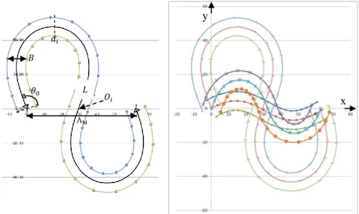
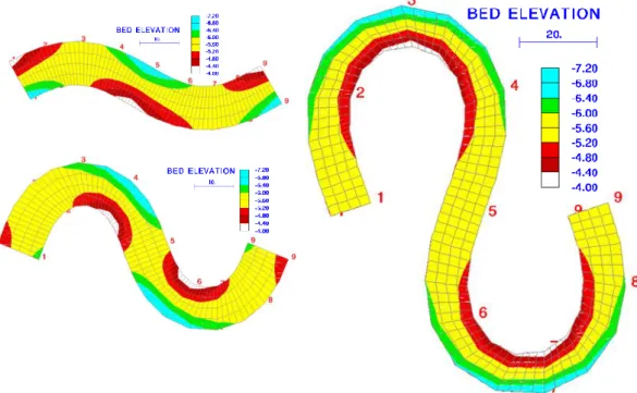
(12) Thèse de Dwinanti Rika Marthanty, Lille 1, 2016. TABLE OF FIGURES Figure 1-1. Research approaches...................................................................................... 3 Figure 1-2. Logical frame work........................................................................................ 4 Figure 2-1. Scheme of the main processes involved in the meandering dynamics and their interactions (Camporeal, et al., 2007) ...................................................................... 7 Figure 2-2. Schematic representation and location of convergence-divergence flow and bed erosion-deposition zones (da Silva, 2006) ................................................................. 9 Figure 2-3. Sketch of flow mechanisms within flooded meandering channels (a) strong floodplain flow (Ervine, et al., 1993), and (b) weak floodplain flow (Wormleaton & Ewunetu, 2006). ............................................................................................................. 11 Figure 2-4. Flow in river bends (Julien, 2002). .............................................................. 12 Figure 2-5. (a) Coordinate systems and (b) secondary flows in a curved channel (Wu, 2008)............................................................................................................................... 13 Figure 2-6. Basic characteristics meandering process .................................................... 13 Figure 3-1. Definition sketch of a meander geometry and bed depth contour. Unit in x and y directions are in meters ......................................................................................... 29 Figure 3-2. Meshing elements, bed depth contours and continuity lines for deviation angles: (a) 30°, (b) 70°, and (c) 110°.............................................................................. 30 Figure 3-3. RMA-10 input setting for meander with deviation angle 30°, and hydrograph inflow .......................................................................................................... 34 Figure 3-4. RMA-11 input setting for meander with deviation angle 30° ..................... 36 Figure 3-5. Cohesive sediment parameters in R4Q file.................................................. 37 Figure 3-6. Non-cohesive sediment parameters in R4Q file .......................................... 38 Figure 3-7. Flow structures ............................................................................................ 40 Figure 3-8. Bed depths ................................................................................................... 44 Figure 3-9. Non-cohesive (Sand) sediment concentrations ............................................ 45 Figure 3-10. Flow convergence-divergence zones schematic representation (a and b), and measured bed topography illustration by (c) Makaveyev (1975) and (d) Jackson (1975) (da Silva, 2006) ................................................................................................... 47 Figure 3-11. Flow structures in small deflection angle channel (a) computed by RMA, (b) run ME-2 measured by Hasegawa (1983), and (c) run RUN30-1 measured by Xu and Bai (2013) ................................................................................................................ 48 Figure 3-12. Flow structures in large deflection angle channel (a) computed by RMA, and (b) run RUN110-2 measured by Xu and Bai (2013) ............................................... 49 Figure 3-13. Flow structures in small deflection angle channel (a) computed by RMA, and (b) test case ME-2 Hasegawa (1983) by Dai (2008) ............................................... 50 Figure 3-14. Flow structures in medium deflection angle channel (a) computed by RMA, and (b) test case #3 Binns (2006) by Dai (2008) ................................................. 51 Figure 3-15. Flow structures in large deflection angle channel (a) computed by RMA, and (b) test case Termini (1996) by Dai (2008) ............................................................. 52 Figure 4-1. Smoothing kernel functions: poly6 (w8(r)), spiky (w9(r)), viscosity (w10(r)) ........................................................................................................................................ 58 Figure 5-1. Process description for (a) the general algorithm, and (b) collision handling algorithm ........................................................................................................................ 63 Figure 5-2. Fluid flow program flow chart ..................................................................... 65 Figure 5-3. Runtime versus particle number .................................................................. 67. xi Universitas Indonesia – Université de Lille 1 © 2016 Tous droits réservés.. lilliad.univ-lille.fr.

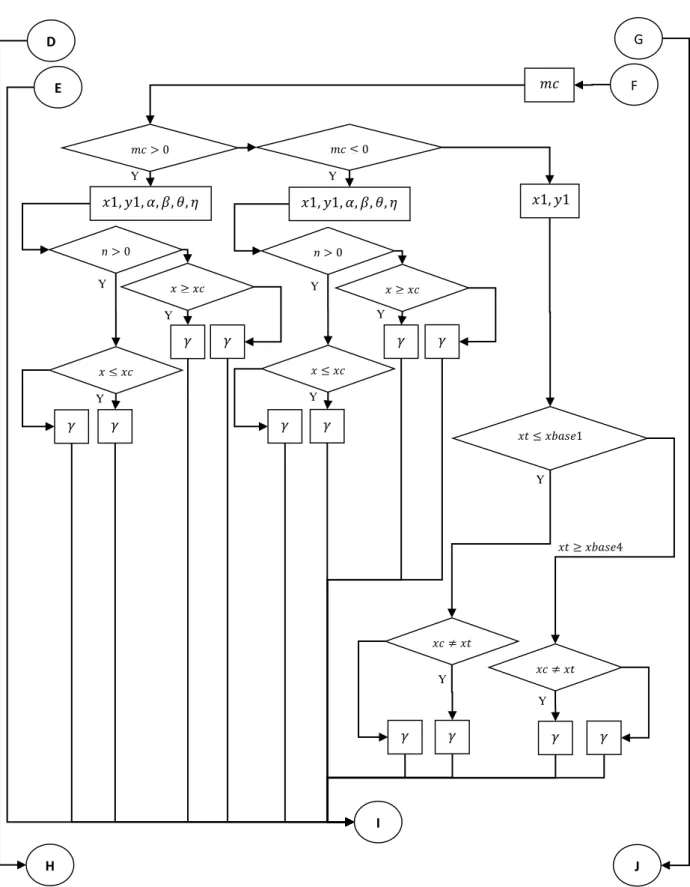
(13) Thèse de Dwinanti Rika Marthanty, Lille 1, 2016. Figure 5-4. At t = 100 𝑑𝑡, (a) Density Response (left to right) Due to the Difference of Rest Density 100 kg/m3, 1000 kg/m3, 10000 kg/m3; (b) Pressure Response (left to right) Due to the Difference of Rest Density 100 kg/m3, 1000 kg/m3, 10000 kg/m3 ............... 67 Figure 5-5. At t = 100 𝑑𝑡, (a) Density Response (left to right) Due to the Difference of Initial Velocity (vx = 10 m/s, vy = 10 m/s, vz = 10 m/s; (b) Pressure Response (left to right) Due to the Difference of Rest Initial Velocity (vx = 10 m/s, vy = 10 m/s, vz = 10 m/s .................................................................................................................................. 68 Figure 5-6. Particle interactions with plane area ............................................................ 69 Figure 5-7. Particle interactions with cylindrical wall ................................................... 70 Figure 5-8. Boundary conditions for a curved channel .................................................. 71 Figure 5-9. Particle interactions with curved channel flow chart (part 1 of 4) ............... 74 Figure 5-10. Initial condition for particle interactions with curved channel plan and 3D view ................................................................................................................................ 77 Figure 5-11. Checking angle refraction for a particle interaction in a curved channel plan view with gravity presence (upper row), and gravity absence (lower row) ........... 78 Figure 5-12. Angle refraction for a particle interaction in a curved channel 3D view with gravity presence (left), and gravity absence (right) ........................................................ 79 Figure 5-13. Transient inviscid flow simulation at t = 15 s in a curved channel plan view with gravity presence (left), and gravity absence (right) ....................................... 80 Figure 5-14. Transient inviscid flow simulation at t = 15 s in a curved channel 3D view with gravity presence (upper), and gravity absence (lower) .......................................... 80 Figure 5-15. Viscous velocity profile (left) at z = 0.667 meter, (right) at x = 0.50 meter ........................................................................................................................................ 81 Figure 5-16. Transient viscous flow simulation at t = 15 s in a curved channel plan view with gravity (left) presence, and (right) absence ............................................................ 82 Figure 5-17. Transient viscous flow simulation at t = 15 s in a curved channel 3D view with gravity (upper) presence, and (lower) absence ....................................................... 82 Figure 5-18. Viscous velocity profile in [m/s] (left) at z = 0.667 meter, (middle) y = 0.5 meter, and (right) at x = 0.50 meter................................................................................ 83 Figure 5-19. Transient viscous vorticity flow simulation at t = 15 s in a curved channel plan view with gravity (left) presence, and (right) absence ........................................... 83 Figure 5-20. Transient viscous vorticity flow simulation at t = 15 s in a curved channel 3D view with gravity (upper) presence, and (lower) absence ........................................ 84 Figure 5-21. Flow simulation with 1% of gravity magnitude in plan view (left) with vorticity, and (right) without vorticity ............................................................................ 85 Figure 5-22. Flow simulation with 1% of gravity magnitude in 3D view (upper) with vorticity, and (lower) without vorticity .......................................................................... 85 Figure 5-23. Flow simulation with 100 times of viscosity, mass, and surface tension magnitude in plan view (left) with vorticity, and (right) without vorticity .................... 86 Figure 5-24. Flow simulation with 100 times of viscosity, mass, and surface tension magnitude in 3D view (left) with vorticity, and (right) without vorticity ...................... 86 Figure 5-25. Particle flows with water properties from t = 0, 3, 6, 9, 12, and 15 second (from upper left in clockwise direction); colors represent velocity [m/s] ...................... 87 Figure 5-26. Particles collision handling (upper left) with gravity, (upper right) with 1% * gravity, (lower left) without gravity, and (lower right) with 10% mass; colors represent velocity [m/s] .................................................................................................. 88 Figure 5-27. Particles collision handling in curved channel with 1% gravity, initial inviscid flow, time 14 seconds in 3D view, time step 1 s, each color represents velocity [m/s] ............................................................................................................................... 91 xii Universitas Indonesia – Université de Lille 1 © 2016 Tous droits réservés.. lilliad.univ-lille.fr.

(14) Thèse de Dwinanti Rika Marthanty, Lille 1, 2016. Figure 5-28. Particles collision handling in curved channel with 1% gravity, initial inviscid flow, time 14 seconds for cross sections at the hemispheres ............................ 92 Figure 5-29. Particles collision handling in curved channel with 1% gravity, initial vorticity flow, time 6.5 seconds in 3D view, time step 0.5 s, each color represents velocity [m/s] .................................................................................................................. 93 Figure 5-30. Particles collision handling in curved channel with 1% gravity, initial vorticity flow, time 6.6 seconds for cross sections at the hemispheres .......................... 94 Figure 5-31. Particles collision handling with curved channel with 1% gravity, initial viscous flow, time 15 seconds in 3D view, time step 1 s, color represents velocity [m/s] ........................................................................................................................................ 95 Figure 5-32. Particles collision handling with curved channel with 1% gravity, initial viscous flow, time 15 seconds for cross sections at the hemispheres ............................. 96 Figure 5-33. Particles collision handling with curved channel with 1% gravity, initial viscous vorticity flow, time 8 seconds in 3D view, time step 0.5 s, color represents velocity [m/s] .................................................................................................................. 97 Figure 5-34. Particles collision handling with curved channel with 1% gravity, initial viscous vorticity flow, time 8 seconds for cross sections at the hemispheres ................ 98 Figure 5-35. Helical formation with initial vorticity viscous flow simulation at t = 6.5 seconds; colors represent velocity [m/s]......................................................................... 99 Figure 5-36. Helical formation with SPH simulation, initial vorticity viscous flow, and results at t = 2.35 seconds; colors represent velocity [m/s].......................................... 100 Figure 5-37. Checking angle refraction for a particle interaction; colors represent velocity [m/s] ................................................................................................................ 101 Figure 5-38. Particles value of: (a) velocity [m/s], (b) pressure [Pa], and (c) density [kg/m3] .......................................................................................................................... 101 Figure 5-39. Helical formation with RMA simulation at t = 1.5 seconds; colors represent velocity [m/s] ................................................................................................ 102 Figure 5-40. Helical formation from experiment investigation of flow structures (Wang & Liu, 2015) ................................................................................................................. 102 Figure 5-41. Theoretical sketch of helical flows in a curved channel, modified from “flow structure past flood channel facility meanders” (Wormleaton & Ewunetu, 2006) ...................................................................................................................................... 103. LIST OF TABLE Table 3-1. Construction of input files (modified from King 1993) ................................ 28 Table 3-2. Variables of meander geometry. ................................................................... 30 Table 3-3. Continuity lines coordinates at meander center lines .................................... 31 Table 3-4. Cross sections from upstream (1) to downstream (9). .................................. 41 Table 3-5. Bed Shear Stress ........................................................................................... 43 Table 5-1. Parameter properties ..................................................................................... 66 Table 5.2. Simulation Cases ........................................................................................... 89. xiii Universitas Indonesia – Université de Lille 1 © 2016 Tous droits réservés.. lilliad.univ-lille.fr.

(15) Thèse de Dwinanti Rika Marthanty, Lille 1, 2016. xiv Universitas Indonesia – Université de Lille 1 © 2016 Tous droits réservés.. lilliad.univ-lille.fr.

(16) Thèse de Dwinanti Rika Marthanty, Lille 1, 2016. 1 INTRODUCTION 1.1. RATIONAL M. S. Yalin defines meandering as “self-induced plan deformation of a. stream that is (ideally) periodic and anti-symmetrical with respect to an axis, x say, which may or may not be exactly straight” (Yalin, 1992). Meanders occur even without sediment transport, it is caused by a large-scale turbulence (da Silva, 2006), turbidity current as in submarine meanders (Darby & Peakall, 2012), and trailing vortices as in low-frequency meander in wind tunnels (Beresh, et al., 2010). Characteristics of flow in meanders are three-dimensional (3D), turbulent, and the presents of helical flow (Wu, 2008). Meandering channels research in general separated, but still correlated, into two approaches: geomorphologic and fluid dynamics, where 3D flow modeling receive more attention for its ability to simulate helicoidal motion even though it is high in computational efforts and limited to simple geometry (Camporeal, et al., 2007). However computer’s capability is growing hence meandering channel can be simulated with a powerful computational fluid dynamics (CFD) tools such as direct numeric simulation (DNS), large eddy simulation (LES), or 𝜅 − 𝜖 models (Wormleaton & Ewunetu, 2006). CFD is traditionally using grid-based numerical methods, such as finite element methods (FEM) and finite volume methods (FVM), which have gained high acceptance ( (Bates, et al., 2005), and (Wendt, 2009)). One developed model with a finite element methods for three-dimensional flow is called Resource Modelling Associates (RMA), to model; density stratified flow (RMA-10), and water quality in estuaries and streams (RMA-11) ( (King, 2013), (King, 2012), and (King, 1993)). It is suited for computing the hydrodynamics of shallow water flow and limited to uniform sediment (Papanicolaou, et al., 2008). In spite of its success, grid-based method has limitations whenever dealing with free surface, deformable boundary, moving interface, and extremely large deformation and crack propagation because of the use of mesh. Complex geometry problems make generating mesh is hard, expensive, and laborious (Liu. 1 Universitas Indonesia – Université de Lille 1 © 2016 Tous droits réservés.. lilliad.univ-lille.fr.

(17) Thèse de Dwinanti Rika Marthanty, Lille 1, 2016. & Liu, 2010). Meshfree methods has been emerged as an alternative grid based methods to deliver better accuracy and stability numerical solutions for PDEs with all possible boundary conditions using particles (Liu & Liu, 2003). Smoothed particle hydrodynamics (SPH) is one most noticeable meshfree method and now become very popular, particularly for free surface flows, it is a robust and powerful method for describing deforming media (Gomez-Gesteira, et al., 2010). SPH main appeals are its ability to predict highly strained motions based on a set of particles, and its consistency with Lagrangian and Hamiltonian mechanics in terms of conservativity (Violeau, 2012). SPH applications for incompressible or nearly incompressible flow in the last two decades is diverse involving dam breaks and plunging waves, gravity currents and multifluid phenomenon, bodies moving in fluids, non-Newtonian fluids, surface tension, and diffusion and precipitation (Monaghan, 2012). Advanced hydraulics with SPH so far has been covered wave action upon waterworks, fish pass, floating oil spill containment boom, and dam spillway (Violeau, 2012). SPH is also a hot topic in Computer Graphics (Kelager, 2006) including realistically animated fluids (Müller, et al., 2003), fluid-fluid interaction (Müller, et al., 2005), hydraulics erosion (Kristof, et al., 2009), and 2D shallow water simulation (Solenthaler, et al., 2011). SPH researches in CFD, hydraulics, and computer graphics mostly do not focus on flow structures except in turbulence. Thus, SPH is a very promising method to answer 3D flow modeling in meander dynamics. 1.2. RESEARCH OBJECTIVES Helical flow patterns from flow simulation with 3D nearly incompressible. flow SPH method is comparable to flow simulation with 3D stratified flow finite element method. 1.3. RESEARCH APPROACHES This research comprises two big parts; (1) modeling meander dynamics with. RMA (Resources Model Association), a 3D stratified flow finite element model, to determine its basic characteristics, and (2) development smoothed particle. 2 Universitas Indonesia – Université de Lille 1 © 2016 Tous droits réservés.. lilliad.univ-lille.fr.

(18) Thèse de Dwinanti Rika Marthanty, Lille 1, 2016. hydrodynamics (SPH) method for 3D nearly incompressible flow to simulate helical flow in a curved channel. Approaches used in part (1) are: 1) modeling sediment transport due to helical flow in meandering river, 2) investigating channel geometries and its relation to the development of helical flows, 3) predicting location of convergence-divergence flow zones and erosion and deposition zones, 4) simulating sediment transport process due to coherent structures and burst in meandering river, and 5) modeling eroding process as mechanical interaction fluid-soil at river bank.. modeling sediment transport due to helical flow in meandering river. investigating channel geometries and its relation to the development of helical flows. predicting location of convergence-divergence flow zones and erosion and deposition zones. simulating sediment transport process due to coherent structures and burst in meandering river. modeling eroding process as mechanical interaction fluidsoil at river bank. Figure 1-1. Research approaches. In part (2), development a FORTRAN code of SPH procedure to simulate helical flow in curved channel follows a logical frame work as in Figure 1-2.. 3 Universitas Indonesia – Université de Lille 1 © 2016 Tous droits réservés.. lilliad.univ-lille.fr.

(19) Thèse de Dwinanti Rika Marthanty, Lille 1, 2016. Physical phenomenon is interpreted in mathematical formulation and represented as governing equations. Numerical method is chosen to find the equations solutions. Algorithm is developed to express the work flow and written in program code. The program run through evaluation until produce results as we expect. If the solutions do not satisfy the objective of the program development, then we have to adjust the parameter. If the solutions do satisfy, then we interpret the results. From result interpretation we can verify and/or validation. According to ISO 9001:2000 section 7.3, designs need to be verified and validated. Verification is defined as the conformation that a product meets identified specifications, and validation is the conformation that a product appropriately meets its design function or the intended use.. physical phenomenon mathematical interpretation mathematical representation numerical approach algorithm development code writing program running Parameter adjustment program evaluation No Solutions Yes Result interpretation Verification and/or validation. Figure 1-2. Logical frame work. 4 Universitas Indonesia – Université de Lille 1 © 2016 Tous droits réservés.. lilliad.univ-lille.fr.

(20) Thèse de Dwinanti Rika Marthanty, Lille 1, 2016. 1.4. RESEARCH LIMITATION This research is limited to: 1) 3D stratified flow finite element method with RMA based on shallow water approach 2) turbulence closure with Smagorinsky closure in RMA-10 model 3) non-cohesive sediment transport in RMA-11 model 4) sine-generated curves for meander geometry representative with RMA model 5) 3D nearly compressible flow for SPH model development 6) turbulence and sediment transport that are not considered yet 7) a curved channel as meander geometry representation with SPH model 8) verification by comparing the results to experimental researches of Hasegawa (1983), Xu & Bai (2013), and Wang & Liu (2015).. 1.5. WRITING LAYOUT This dissertation writing is divided into two parts in general. The first one is. to model meander dynamics with RMA-10 AND RMA-11 to determine its basic characteristics, and written in chapter 2 and 3. This part is prepared in Laboratoire de Génie Civil et géo-Environnement, Ecole Polytechnique de Lille, Université de Lille 1, France. The last one is to develop smoothed particle hydrodynamics (SPH) method to simulate helical flow in a curved channel, and presented in chapter 4 and 5. This part is done in Laboratory of Hydraulics, Hydrology and River, Civil Engineering Department, Universitas Indonesia, Indonesia. Chapter 2 writes about fundamental theory of meandering physical processes, and flow structure, erosion-deposition and bend migration in meandering bends. In the end, this chapter wrap up meandering flow basic characteristics. Chapter 3 presents flow simulations with RMA from description model, model set-up, results and discussion, and lastly results confirmation with other experimental studies in meandering channel. From chapter 2 and chapter 3, we have published (1) a paper in International Conference Sediment Transport Modeling in Hydrological Watersheds and Rivers, Istanbul, Turkey, 2012, titled ‘Developing model to predict curve. 5 Universitas Indonesia – Université de Lille 1 © 2016 Tous droits réservés.. lilliad.univ-lille.fr.

(21) Thèse de Dwinanti Rika Marthanty, Lille 1, 2016. dynamics in river meandering process’; and (2) a paper in Journal of Urban and Environmental Engineering (JUEE) Vol 8, No 2, 2014, titled ‘Assessment of the capability of 3D stratified flow finite element model in characterizing meander dynamics’, DOI: 10.4090/juee.2014.v8n2.155166. Chapter 4 describes SPH method, opening with basic formulation, and closing in procedure formulation. Chapter 5 composes flow simulations with SPH from 3D fluid flow model, numerical simulation, and finally results discussion. Chapter 6 completes this writing by reviewing conclusions, research contributions, and suggestions for future research. Based on chapter 4 and chapter 5, we have published (1) a paper in International Conference on Ecohydrology, Yogyakarta, Indonesia, 2014, titled ‘Reviewing the use of smoothed particle hydrodynamics as a tool in modeling river meandering’, ISBN: 978-979-8163-22-7, and (2) we plan afterwards to publish a paper in an international journal with tentatively title ‘Development of smoothed particle hydrodynamics (SPH) method to simulate helical flow in a curved channel’.. 6 Universitas Indonesia – Université de Lille 1 © 2016 Tous droits réservés.. lilliad.univ-lille.fr.

(22) Thèse de Dwinanti Rika Marthanty, Lille 1, 2016. 2 BASIC CHARACTERISTICS OF MEANDERING DYNAMICS Einstein firstly explained the cause of the formation of meanders in 1926 where streams tend to flow in winding and turning course instead of following the downward slope as a result from Coriolis-force (Einstein, 1926). Even without bends, the circular movement still exists at cross-sections of its course. Meandering is not only happened on alluvial streams but also on melting water channels on ice (Langbein & Leopold, 1966), wind tunnels (Beresh, et al., 2010), and submarine channels (Darby & Peakall, 2012). 2.1. MEANDERING PHYSICAL PROCESSES River is meandering when there is an active process of erosion at the outer. bank and deposition on the inner bank (Raudkivi, 1998). Camporeal et al. (2007) in Figure 2-1 present the main elements of meandering dynamics are curvature and erodible boundary. Each of main elements can drive secondary currents then leads to transversal flow field.. Figure 2-1. Scheme of the main processes involved in the meandering dynamics and their interactions (CAMPOREAL, ET AL., 2007). 7 Universitas Indonesia – Université de Lille 1 © 2016 Tous droits réservés.. lilliad.univ-lille.fr.

(23) Thèse de Dwinanti Rika Marthanty, Lille 1, 2016. 2.2. MEANDERING BENDS In river modeling is often used one-dimensional model due to efficiency and. applied in the study of long-term sedimentation problems in rivers. But flows in curved channels give evidence of complex three-dimensional features that have big influences on sediment transport process. Thus these phenomena must rely on three-dimensional model for all practical purposes. To simulate correctly channel meandering process, at least a model must be capable of; (1) taking into account the helical flow effect, (2) dealing with bank erosion, and (3) coping with the moving boundary problems. Erosion mechanisms vary with bank material. The bank material fails in blocks for a cohesive bank, and it fails in particles for a noncohesive one (Wu, 2008). Here, the river scale is defined as reach scale where the domain is longer than the channel by a factor of at least 5 and up to 50 or more. Considering that reach scale is a common scale in management activities such as scour around bridge piers, in-channel sedimentation process, bank erosion and channel migration, thus it relates the flow and sediment transport around structures, and linkages strongly to morpho-dynamic and habitat process likewise the flow field itself (Bates, et al., 2005). 2.2.1. FLOW STRUCTURES In curved channel, the dispersion transport plays great role due to helical. flow. The existence of helical flow is caused by the difference between the centrifugal forces in the upper and lower layers (Wu, 2008). More fundamental explanation is the physical reasoning of meandering phenomenon. Recent research explained that meandering is caused by the large-scale turbulence where is designated to bursting processes (da Silva, 2006). da Silva and Ahmari (2009) found that the formation of large-scale river forms is directly related to the large-scale turbulence, particularly the formation of alternate bars and meanders through the actions of horizontal coherent structures on the mean flow and the mobile bed and banks (da Silva & Ahmari, 2009). This is agreed with Mao (2003) experiments that at high roughness Reynolds number the bursts and sweeps phenomena can send sediment particles into suspension where bed forms and bed roughness interact with the coherent. 8 Universitas Indonesia – Université de Lille 1 © 2016 Tous droits réservés.. lilliad.univ-lille.fr.

(24) Thèse de Dwinanti Rika Marthanty, Lille 1, 2016. turbulent structures and resulted in flow and sand movement in alluvial rivers (Mao, 2003). The most recent result comes from (Esfahani & Keshavarzi, 2012), they detected the importance of sweeps and bursts on sediment deposition, and stated the occurrence of fluctuating velocities in three-dimensions inside meanders is responsible for sediment transport.. a.. b.. c.. Figure 2-2. Schematic representation and location of convergence-divergence flow and bed erosion-deposition zones (DA SILVA, 2006). If we assume the ratio of channel width to its depth is large, then we can consider the flow in meandering river is vertically averaged and convective as shown by in Figure 2-2 (da Silva, et al., 2006). In the sine-generated channels, da Silva et al. stated that the flow is accelerating where the vertically averaged streamlines are converging to each other, and decelerating where the vertically averaged streamlines are diverging from each other. From their experiments, for small deflection angles (30°) location of maximum erosion-deposition zones near the crossover of the sinuosity, for intermediate deflection angles (70°) location of maximum erosion-deposition zones between the crossover and apex of the sinuosity, and for large deflection angles (110°) location of maximum erosion-. 9 Universitas Indonesia – Université de Lille 1 © 2016 Tous droits réservés.. lilliad.univ-lille.fr.

(25) Thèse de Dwinanti Rika Marthanty, Lille 1, 2016. deposition zones near the apex of the sinuosity. Esfahani & Keshavarzi (2012) investigated different deflection angles affected on fluctuation velocities that is responsible for direction of sediment deviation and then migration pattern. They have the same opinion that convergence-divergence regions coincide with erosion-deposition regions (Esfahani & Keshavarzi, 2012). As erosion-deposition zones coincide with the convergence-divergence flow zones in meandering river, we can predict the zones of convective acceleration and deceleration of flow, and the zones of upward and downward bed displacements by examining velocity, depth distributions, meander wavelength, and plan shape of meandering river ( (Odgaard, 1989) and (da Silva, 2006)). Turbulence consists of coherent (phase-correlated) and phase-random (i.e., incoherent) motions. A coherent structure is a connected, large-scale turbulent fluid mass with a phase-correlated vorticity over its spatial event (Hussain, 1983). Coherent structure is used to point out the largest cluster of turbulent eddies which has the most common sense of rotation. The term burst is to appoint the evolution of coherent structures during its life span (da Silva, 2006). As mentioned by (Sanjou & Nezu, 2009), velocity inflection-point instability, i.e. shear instability, occurs at the meandering entrance, suggesting the generation of a horizontal vortex. Whether such a vortex is surely generated and how it is convected in the meandering channel is not yet clear. The combination between horizontal vortex and secondary currents may promote significant mass and momentum exchanges at the interchanging boundaries near main channel bed and near free surface. Coherent turbulence structures in meanders, bursts and sweeps, are responsible for transferring fluid momentum across local velocity gradients (da Silva & Ahmari, 2009). Bursts are oriented towards inner-bank and sweeps are oriented towards outer-bank of the channel bend (Güneralp, et al., 2012). According to Guneralp et al. (2012), coherent turbulent structures may be regarded as temporal imbalances in the cross-section force equilibrium combined with turbulent structures movement, and changes in the mean cross-section velocity through the water column joined with secondary currents.. 10 Universitas Indonesia – Université de Lille 1 © 2016 Tous droits réservés.. lilliad.univ-lille.fr.

(26) Thèse de Dwinanti Rika Marthanty, Lille 1, 2016. Ervine et al. (1993) shows in Figure 2-2 the importance of flow mechanisms in meandering over-bank flow based on their measurements. From floodplain or outer-bank, flow moves toward main channel as a large secondary flow which is vigorously expulsion of inner-bank. Then secondary flow decays right after bend apex. Afterwards, primary flow proceeds to the next bend, and converges with strong vortex from floodplain.. Figure 2-3. Sketch of flow mechanisms within flooded meandering channels (a) strong floodplain flow (ERVINE, ET AL., 1993), and (b) weak floodplain flow (WORMLEATON & EWUNETU, 2006).. 11 Universitas Indonesia – Université de Lille 1 © 2016 Tous droits réservés.. lilliad.univ-lille.fr.

(27) Thèse de Dwinanti Rika Marthanty, Lille 1, 2016. 2.2.2. EROSION, DEPOSITION AND BEND MIGRATION In theory of river basins, river process can be divided into three main zones;. (1) erosion at the upper zone, (2) transportation at the mid zone, and (3) deposition at the lower zone. As a fluvial system, those zones are characterized by sediment process, bed elevation, channel pattern, slope, and bed material. At the upper zone, it is typically erosion process, degradation bed, confluence channel, steep slope, and bed material of cobble – gravel. At the mid zone, it is commonly transportation process, equilibrium bed, single channel, mild slope, and bed material of gravel – sand. The last part, it is expected sedimentation process, aggradation bed, branching channel, flat slope, and bed material of sand – silt. Alluvial rivers flow with their own deposits. Its equilibrium channel leads to a balance between incoming and outgoing water discharge and sediment load. The cross-sectional geometry may change at local on condition that the deposition volume within a river reach is equal to the erosion volume. Consequently at river bends, its cross-sectional geometry is in equilibrium. Nevertheless, lateral migration of the bend indicates instability of the stream planform geometry (Julien, 2002). Deviation angle 𝜆 depends primarily on the ratio of flow depth to radius of curvature thus sharp bends will exhibit stronger secondary flows (Julien, 2002). It is expressed in: tan 𝜆 =. τr R τθ. a2. h 2m ℎ. = [ Ω (d ) R. s. ]𝑅. (2-1). FIGURE 2-4. FLOW IN RIVER BENDS (JULIEN, 2002).. 12 Universitas Indonesia – Université de Lille 1 © 2016 Tous droits réservés.. lilliad.univ-lille.fr.

(28) Thèse de Dwinanti Rika Marthanty, Lille 1, 2016. Figure 2-5. (a) Coordinate systems and (b) secondary flows in a curved channel (WU, 2008).. 2.3. MEANDERING FLOW BASIC CHARACTERISTICS Development of meander dynamics model has to have a capability to simulate. meander flow characteristic and sediment transport distribution pattern, or at least having the same capability as the finite element method (Wu, 2008). Here, the meander flow is characterized by having helical flow and coherent structures (bursts and sweeps), higher flow velocity at the outer banks and lower in the inner banks, sediment erosion at the outer banks and deposition in the inner banks, higher sediment concentration at the outer banks and lower in the inner banks (da Silva, 2006).. Meander Dynamics Modeling. Flow Structure. Sediment Transport. Morpho-dynamics. Primary Flow. Erosion. Migration. Secondary Flow. Deposition. Expansion. Helical Flow. Scouring. Eddies Horizontal Bursts Sweeps Vertical Bursts Sweeps. Figure 2-6. Basic characteristics meandering process. 13 Universitas Indonesia – Université de Lille 1 © 2016 Tous droits réservés.. lilliad.univ-lille.fr.

(29) Thèse de Dwinanti Rika Marthanty, Lille 1, 2016. 14 Universitas Indonesia – Université de Lille 1 © 2016 Tous droits réservés.. lilliad.univ-lille.fr.

(30) Thèse de Dwinanti Rika Marthanty, Lille 1, 2016. 3 FLOW SIMULATIONS WITH RMA 3.1. NUMERICAL EXPERIMENT WITH RMA (RESOURCES MODELING ASSOCIATIONS) The governing equations of RMA-10 is based on the combination of the. Reynolds form of the Navier-Stokes equations, the volume continuity equation, the advection diffusion equation, and an equation of state relating water density to salinity or temperature. For fully three-dimensional model, the required boundary conditions that must be defined here are water surface elevation, sediment concentration, sediment flux, and specified velocity at land and water boundaries. Practically it can be divided into three categories which are the free surface, the bed, and the side boundaries. The finite element approach in RMA-10 is using iso-parametric approximations to define elements, Galerkin Method of Weighted Residuals for the finite element derivation, Newton-Rhapson method to structure and iterate for the nonlinearity, modified Crank-Nicolson time stepping scheme for unsteady flow, and Gaussian quadrature to integrate the finite element integrals. Hydrostatic pressure assumption is considered since vertical momentum effects may be neglected and the vertical velocities are sufficiently small ( (King, 1993) and (King, 2012)). Here, we used RMA-10 version 87e in 20 November 2012. RMA-11 is a finite element water quality model to simulate threedimensional estuaries, bays, lakes and rivers as separate system or combined form. It employs the input of velocities and depths from RMA-10 for the computation of advection diffusion constituent transport equations with additional terms for each source/sink and growth/decay. 3.1.1. RMA-10 DESCRIPTION MODEL. 3.1.1.1 Governing Equations for Three-Dimensional Stratified Flow RMA-10 uses three-dimensional stratified flow equations describing velocity in all three Cartesian directions, water pressure and the distribution of constituent concentration of sediment throughout the system. The sediment is treated as the dependent variable.. 15 Universitas Indonesia – Université de Lille 1 © 2016 Tous droits réservés.. lilliad.univ-lille.fr.

(31) Thèse de Dwinanti Rika Marthanty, Lille 1, 2016. Hydrodynamics. approximation,. or. often. called. shallow. water. approximation, is widely used in surface water systems. Shallow water (or long wave) approximation assumes that ratio between horizontal (L) to vertical (L) scales is very large, or. 𝐻 𝐿. ≪ 1 (Ji, 2008).. ∂u. Volume Continuity: ∂xj = 0. (3-1). Momentum equation:. (3-2). j. 𝜕𝑢. 𝜕𝑢. 𝜕. 𝜕𝑢. 𝜕𝑝. 𝜌 ( 𝜕𝑡𝑖 + 𝑢𝑗 𝜕𝑥 𝑖 ) − 𝜕𝑥 (𝜀𝑥𝑖 𝑥𝑗 𝜕𝑥 𝑖 ) + 𝜕𝑥 − Γ𝑥𝑖 = 0 𝑗. 𝑗. 𝜕𝑐. 𝑗. 𝜕𝑐. 𝑖. 𝜕. 𝜕𝑐. Advection Diffusion: 𝜕𝑡 + 𝑢𝑗 𝜕𝑥 − 𝜕𝑥 (𝐷𝑥𝑗 𝜕𝑥 ) − 𝜃𝑠 = 0 𝑗. 𝑗. (3-3). 𝑗. 𝜕𝑝. Hydrostatic Approximation: 𝜕𝑧 + 𝜌𝑔 = 0. (3-4). where 𝑖, 𝑗 are general coordinate directions as subscripts, 𝑢𝑗 is the component vector velocity in 𝑗-direction, 𝑥𝑗 is coordinate system in 𝑗-directions, 𝜌 is density, 𝜺𝒙𝒊 𝒙𝒋 is the turbulent eddy coefficients, 𝑢𝑖 is the vector velocity in 𝑖-direction, 𝑡 is for time, 𝑝 is for pressure, Γx is external forces, 𝑐 is constituent concentration, 𝐷𝑥 is the eddy diffusion coefficients, and 𝜃𝑠 is the source/sink for the constituent. In the RMA-10 formulation of the vertical velocity 𝑤 is used only in the two momentum equations and the advection diffusion equation. For the simulation model, the main dependent variables are thus the horizontal velocity components 𝑢 and 𝑣, the water depth ℎ and the constituent concentration 𝑐. For equations (1) through (4), the geometric system varies with time where the water depth ℎ varies during the simulation. In modifying the geometry the transformation is defined by 𝑎 as the elevation of the bottom relative to the same vertical datum and 𝑏 as the fixed vertical location to which the water surface will be transformed. To add in the impact of the transformation, the horizontal eddy coefficients have been modified but neglected the influence of slightly non horizontal diffusion induced by the transformation. The final form for three-dimensional stratified flow that is used in RMA-10 are momentum equations (5) and (6), volume continuity equation (7), advection diffusion equation (8), and equation of state (9):. 16 Universitas Indonesia – Université de Lille 1 © 2016 Tous droits réservés.. lilliad.univ-lille.fr.

(32) Thèse de Dwinanti Rika Marthanty, Lille 1, 2016. 𝜕𝑢. 𝜕𝑢. 𝜕𝑢. 𝜕𝑢. (3-5). 𝜌 {ℎ 𝜕𝑡 + ℎ𝑢 𝜕𝑥 + ℎ𝑣 𝜕𝑦 + 𝜕𝑧 [(𝑏 − 𝑎)(𝑤 − 𝑢𝑇𝑥 − 𝑣𝑇𝑦 ) − (𝑧 − 𝑎) (𝑏 − 𝑎). 𝜕ℎ 𝜕𝑡 𝜕. 𝜕. ℎ. 𝜕𝑢. 𝜕𝑧. 𝜕𝑢. 𝜕. ℎ. 𝜕𝑢. ]} − (𝑏 − 𝑎) 𝜕𝑥 [𝜺𝑥𝑥 (𝑏−𝑎) 𝜕𝑥 ] − (𝑏 − 𝑎) 𝜕𝑦 [𝜺𝑥𝑦 (𝑏−𝑎) 𝜕𝑦] − 𝜕𝑎. 𝜕ℎ. [𝜺𝑥𝑧 𝜕𝑧 ] + 𝜌𝑠 𝑔ℎ 𝜕𝑥 + 𝜌𝑠 𝑔ℎ 𝜕𝑥 + 𝑔𝑥 ℎ − ℎ𝛤𝑥 = 0. 𝜕𝑣. 𝜕𝑣. 𝜕𝑣. 𝜕𝑣. (3-6). 𝜌 {ℎ 𝜕𝑡 + ℎ𝑢 𝜕𝑥 + ℎ𝑣 𝜕𝑦 + 𝜕𝑧 [(𝑏 − 𝑎)(𝑤 − 𝑢𝑇𝑥 − 𝑣𝑇𝑦 ) − (𝑧 − 𝑎) (𝑏 − 𝑎). 𝜕ℎ 𝜕𝑡 𝜕. 𝑏 𝜕𝑢. 𝑣𝑠. ∂(a+h) ∂y. 𝜕𝑣. 𝜕. ℎ. 𝜕𝑣. 𝜕𝑎. 𝜕ℎ. [𝜺𝑦𝑧 𝜕𝑧 ] + 𝜌𝑠 𝑔ℎ 𝜕𝑦 + 𝜌𝑠 𝑔ℎ 𝜕𝑦 + 𝑔𝑦 ℎ − ℎ𝛤𝑦 = 0. (𝑏−𝑎) 𝜕𝑢. 𝑇 𝜕𝑧 𝑥. ℎ. ∂(a). − 𝑣𝑏. 𝜕𝑐. ℎ. 𝜕𝑣. 𝜕𝑧. ∫𝑎 [𝜕𝑥 −. 𝜕. ]} − (𝑏 − 𝑎) 𝜕𝑥 [𝜺𝑦𝑥 (𝑏−𝑎) 𝜕𝑥] − (𝑏 − 𝑎) 𝜕𝑦 [𝜺𝑦𝑦 (𝑏−𝑎) 𝜕𝑦] −. ∂y. 𝜕𝑐. 𝜕𝑢. + 𝜕𝑦 −. (𝑏−𝑎) 𝜕𝑣 ℎ. 𝑇 ] 𝑑𝑧 𝜕𝑧 𝑦. + 𝑢𝑠. ∂(a+h) ∂x. − 𝑢𝑏. ∂(a) ∂x. +. (3-7). 𝜕ℎ. (3-8). 𝜕ℎ. + 𝜕𝑡 = 0 𝜕𝑐. 𝜕𝑐. ℎ 𝜕𝑡 + ℎ𝑢 𝜕𝑥 + ℎ𝑣 𝜕𝑦 + 𝜕𝑧 [(𝑏 − 𝑎)(𝑤 − 𝑢𝑇𝑥 − 𝑣𝑇𝑦 ) − (𝑧 − 𝑎) 𝜕𝑡 ] − (𝑏 − 𝑎) 𝜕. 𝜕. ℎ. 𝜕𝑐. 𝜕. ℎ. 𝜕𝑐. (𝐷𝑥 (𝑏−𝑎) 𝜕𝑥) − (𝑏 − 𝑎) 𝜕𝑦 (𝐷𝑦 (𝑏−𝑎) 𝜕𝑦) − (𝑏 − 𝜕𝑥 𝜕𝑐. 𝑎) 𝜕𝑧 (𝐷𝑧 𝜕𝑧) − ℎ𝜃𝑠 = 0 𝜌 − 𝐹(𝑐) = 0. (3-9). where 𝜌𝑠 is the density at the surface; 𝜌𝑧 is the density at the elevation 𝑧; 𝑢𝑠 and 𝑣𝑠 are horizontal Cartesian velocity components at the water surface; and 𝑢𝑏 and 𝑣𝑏 are horizontal Cartesian velocity components at the bed. It is noted that the momentum and advection diffusion equations have been multiplied by ℎ. 𝐷𝑥 , 𝐷𝑦 , and 𝐷𝑧 represent similar approximations for the diffusion coefficients to those were made for the eddy coefficients. 𝑇𝑥 , 𝑇𝑦 , 𝑔𝑥 , and 𝑔𝑦 are defined by: 𝜕𝑎. (𝑧−𝑎) 𝜕ℎ. ℎ. 𝜕𝑎. (𝑧−𝑎). 𝜕𝑎. (3-10). 𝜕𝑎. (𝑧−𝑎) 𝜕ℎ. ℎ. 𝜕𝑎. (𝑧−𝑎). 𝜕𝑎. (3-11). 𝑇𝑥 = 𝜕𝑥 + (𝑏−𝑎) 𝜕𝑥 − (𝑏−𝑎) 𝜕𝑥 + (𝑏−𝑎)2 ℎ 𝜕𝑥. 𝑇𝑦 = 𝜕𝑦 + (𝑏−𝑎) 𝜕𝑦 − (𝑏−𝑎) 𝜕𝑦 + (𝑏−𝑎)2 ℎ 𝜕𝑦 𝑎+ℎ 𝜕. 𝑔𝑥 = ∫𝑧. 𝜕𝑥. 𝑎+ℎ 𝜕. 𝑔𝑦 = ∫𝑧. 𝜕𝑦. (𝜌𝑔) 𝑑𝑧. (3-12). (𝜌𝑔) 𝑑𝑧. (3-13). 17 Universitas Indonesia – Université de Lille 1 © 2016 Tous droits réservés.. lilliad.univ-lille.fr.

(33) Thèse de Dwinanti Rika Marthanty, Lille 1, 2016. 3.1.1.2 Boundary Conditions and Surface Tractions The free water surface is no leakage boundary conditions across the surface and zero pressure where the water depth is 𝒉. 𝑤𝑠 =. 𝑑ℎ. (3-14). 𝑑𝑡. The bottom is no leakage condition with drag from the bed for velocities: 𝜕𝑎. 𝜕𝑎. (3-15). 𝑢𝑏 𝜕𝑥 + 𝑣𝑏 𝜕𝑦 − 𝑤𝑏 = 0. where 𝑢𝑏 , 𝑣𝑏 and 𝑤𝑏 are represent Cartesian velocity components at the bottom, and 𝑎 is the elevation of the bottom relative to the same vertical datum. The side boundaries occur at system cuts where the boundary conditions specify water surface elevations for each (𝑥, 𝑦) location, velocities at the (𝑥, 𝑦, 𝑧) location, or flows at the cuts (𝑢ℎ and or 𝑣ℎ). The boundary is considered as being at a fixed location, thus it will require special numerical and analytical techniques for moving boundary systems. Hence, in the future paper we will propose the additional technique to simulate curve dynamic evolvement due to erosion and disposition process. Surface tractions for bed friction are using Chezy friction equation: 𝛤𝑥 = −. 𝜌𝑔𝑢𝑏 𝑉 𝐶2. , 𝛤𝑦 = −. 𝜌𝑔𝑣𝑏 𝑉. (3-16). 𝐶2. where 𝜌 is density, 𝑔 is gravity acceleration, 𝑢𝑏 and 𝑣𝑏 are represent Cartesian velocity components at the bottom, 𝑉 = (𝑢𝑏 2 + 𝑣𝑏 2 )0.5 is magnitude of water velocity at the bed, and 𝐶 is Chezy friction coefficient. Likewise, the wall friction is computed analogues to bed friction and directed in against the flow.. 3.1.1.3 Eddy Viscosity and Diffusivity in The Vertical Direction Vertical eddy viscosity and diffusivity may vary significantly over the depth in both homogeneous and stratified flow. RMA-10 has been developed to permit various forms of the dependence of these parameters. Parametric description for horizontal eddy viscosity and diffusivity 𝜺𝑥𝑧 , 𝜺𝑦𝑧 , and 𝐷𝑧 are defined as quadratically varying over the depth. (𝑧−𝑎). (𝑧−𝑎). 𝜺𝑥𝑧 = 𝜺𝑥𝑧 ′ [𝐸𝐷𝐷1 + (𝑏−𝑎) (𝐸𝐷𝐷2 + (𝑏−𝑎) 𝐸𝐷𝐷3)]. (3-17). where 𝜺𝑥𝑧 ′ , 𝐸𝐷𝐷1, 𝐸𝐷𝐷2, and 𝐸𝐷𝐷3 are fixed parameters defined in the model input. Similar way of scaling factors are used for 𝜺𝑦𝑧 and 𝐷𝑧 . 18 Universitas Indonesia – Université de Lille 1 © 2016 Tous droits réservés.. lilliad.univ-lille.fr.

(34) Thèse de Dwinanti Rika Marthanty, Lille 1, 2016. RMA-10 formulation for vertical eddy viscosity and diffusivity is based on diffusivity distributions developed for stratified reservoirs application. The 𝜺𝑥𝑧 , 𝜺𝑦𝑧 , and 𝐷𝑧 are scaled from the homogeneous values developed using 2.63. 𝐷𝑓 is the defined factor and applied to all three coefficients, and in English unit where 𝐷𝑓 = 1.0; 𝜺𝑥𝑧 ′′ = 𝐷𝑓 𝜺𝑥𝑧 when. 1 𝜕𝜌. (3-18). < 𝐷𝑐𝑟 then 𝐷𝑓 = 0.6888 ∗ 10−4 ∗ (−. 𝜌 𝜕𝑧. 1 𝜕𝜌 0.7 𝜌 𝜕𝑧. ). 1 𝜕𝜌. (3-19). when 𝜌 𝜕𝑧 > 𝐷𝑐𝑟 then 𝐷𝑐𝑟 = 1.1335 ∗ 10−6 ft-1. (3-20). if 𝐷𝑓 < 0.01 then 𝐷𝑓 = 0.01. (3-21). 𝜕𝜌. (3-22). if 𝜕𝑧 > 0 then 𝐷𝑓 = 50.0. The value from this method must be in the input data for homogeneous flow. Metric units can be used with the appropriate scaling. Horizontal and vertical eddy diffusivity coefficients are used as turbulence mixing parameters in in hydrodynamics model (Ji, 2008). The horizontal eddy viscosity is related to turbulence in flow and affects velocity distribution. Smagorinsky formula can used to calculate horizontal eddy viscosity. In the model, RMA-10 uses Smagorinsky closure to control turbulence.. 3.1.1.4 Solution of The Continuity Equation for Vertical Velocities Volume continuity equation (1) is converted into a boundary value problem and differentiated with respect to 𝑧. It is subjected to boundary conditions for the water surface and the bed. ∂2 w ∂z2. ∂. ∂u. ∂v. (3-23). = − ∂z ( ∂x + ∂y). 𝑤 = 𝑢∗. 𝑑(ℎ+𝑎) 𝑑𝑥 𝑑𝑎. + 𝑣∗ 𝑑𝑎. 𝑤 = 𝑢∗ 𝑑𝑥 + 𝑣 ∗ 𝑑𝑦. 𝑑(ℎ+𝑎) 𝑑𝑦. 𝑑ℎ. + 𝑑𝑡. at the water surface. (3-24). at the bed. (3-25). In these equations the values of 𝑢 and 𝑣 will be known at all locations from the previous part of the solution step. Then values obtained for 𝑤 in this solution are used in the next iteration for 𝑢, 𝑣, ℎ and 𝑠.. 19 Universitas Indonesia – Université de Lille 1 © 2016 Tous droits réservés.. lilliad.univ-lille.fr.

(35) Thèse de Dwinanti Rika Marthanty, Lille 1, 2016. 3.1.2. EQUATIONS OF STATE Equations of state are required to described the relationships of the. constituent concentration such suspended sediment, temperature, and salinity to density in the RMA-10 equations. These equations are empirical. Suspended sediment: 𝜌 = 1.940 ∗ (1.0 + 2.4 ∗ 10−6 𝑠𝑠) where 𝑠𝑠 in. (3-26). mg/l 𝜌 = 1.93993 + 𝑇 ∗ (5.88599 ∗ 10−5 − 1.108539 ∗. Temperature:. (3-27). 10−5 ∗ 𝑇) where 𝑇 in degrees C (4.906∗𝑠−11.7). Salinity: 𝜌 = 1.940 ∗ {1.0 + (6511.7−1.906∗𝑠)} where 𝑠 in parts per. (3-28). thousands It is noted that suspended sediment is treated as a conservative constituent. Settling, bed erosion, and deposition are not incorporated into RMA-10 module computation. In one simulation when multiple constituents are used, then density is defined as 1.940 added to the discrepancy from 1.940 for each constituent.. 3.1.3. RMA-11 DESCRIPTION MODEL. 3.1.3.1 Governing Equations for Three-Dimensional Transport The RMA-11 governing equations are continuity equation (3-29) and advection diffusion equation (3-30). The advection diffusion equations in both conservative and non-conservative forms are presented in generalized form where source/sink and reactions variables are represented by generic terms. The same manner with RMA-10 governing equations that they are transformed to a constant water surface elevation 𝑏, and in the case where the principal diffusion direction is at angle to the 𝑥 axis. 𝜕𝑢. 𝜕𝑣. 𝜕𝑤. 𝜕𝑢. 𝜕𝑣. ℎ (𝜕𝑥 + 𝜕𝑦) + (𝑏 − 𝑎) 𝜕𝑧 − (𝑏 − 𝑎) (𝑇𝑥 𝜕𝑧 + 𝑇𝑦 𝜕𝑧 ) − ℎ𝑞0 = 0 𝜕𝑐. ℎ 𝜕𝑡 + ℎ. 𝜕(𝑢𝑐) 𝜕𝑥. 𝜕(𝑣𝑐). (𝑏 − 𝑎)𝑇𝑦 𝜕. 𝜕𝑧. (𝑏−𝑎). ℎ 𝜕𝑥 (. ℎ. (𝑏 − 𝑎)𝑇𝑥. +ℎ. 𝜕(𝑣𝑐) 𝜕𝑦. + (𝑏 − 𝑎). 𝜕(𝑤𝑐). 𝜕ℎ 𝜕𝑐. 𝜕. 𝜕𝑧. − (𝑏 − 𝑎)𝑇𝑥 𝜕𝑐. 𝜕(𝑢𝑐) 𝜕𝑧. (3-29) (3-30). −. 𝜕𝑐. − (𝑧 − 𝑎) 𝜕𝑡 𝜕𝑧 − ℎ 𝜕𝑥 (𝐷𝑥 𝜕𝑥 + 𝐷𝑥𝑦 𝜕𝑦) + 𝜕𝑐. 𝜕. 𝜕𝑐. 𝜕𝑐. {𝐷𝑥 𝑇𝑥 + 𝐷𝑥𝑦 𝑇𝑦 } 𝜕𝑧) + (𝑏 − 𝑎)𝑇𝑥 𝜕𝑧 (𝐷𝑥 𝜕𝑥 + 𝐷𝑥𝑦 𝜕𝑦) − 𝜕. (𝑏−𝑎). ( 𝜕𝑧. ℎ. 𝜕𝑐. 𝜕. 𝜕𝑐. 𝜕𝑐. {𝐷𝑥 𝑇𝑥 + 𝐷𝑥𝑦 𝑇𝑦 } 𝜕𝑧) − ℎ 𝜕𝑦 (𝐷𝑥𝑦 𝜕𝑥 + 𝐷𝑦 𝜕𝑦) +. 20 Universitas Indonesia – Université de Lille 1 © 2016 Tous droits réservés.. lilliad.univ-lille.fr.

(36) Thèse de Dwinanti Rika Marthanty, Lille 1, 2016. 𝜕. (𝑏−𝑎). ℎ 𝜕𝑦 (. ℎ. (𝑏 − 𝑎)𝑇𝑦. 𝜕𝑐. 𝜕. 𝜕𝑐. 𝜕𝑐. {𝐷𝑥𝑦 𝑇𝑥 + 𝐷𝑦 𝑇𝑦 } 𝜕𝑧) + (𝑏 − 𝑎)𝑇𝑦 𝜕𝑧 (𝐷𝑥𝑦 𝜕𝑥 + 𝐷𝑦 𝜕𝑦) − 𝜕. 𝜕𝑧. (𝑏−𝑎). (. ℎ. 𝜕𝑐. 𝜕. {𝐷𝑥𝑦 𝑇𝑥 + 𝐷𝑦 𝑇𝑦 } 𝜕𝑧) − (𝑏 − 𝑎) 𝜕𝑧 (𝐷𝑦. 𝐾ℎ𝑐 − ℎ𝜃𝑠 − (𝑏 − 𝑎). 𝜕(𝑉𝑆 𝑐) 𝜕𝑧. (𝑏−𝑎) 𝜕𝑐 ℎ. 𝜕𝑧. )−. =0. If the continuity equation is substituted into advection diffusion equation then it becomes constituent transport equation: 𝜕𝑐. 𝜕𝑐. 𝜕𝑐. 𝜕ℎ 𝜕𝑐. ℎ 𝜕𝑡 + ℎ𝑢 𝜕𝑥 + ℎ𝑣 𝜕𝑦 + [(𝑏 − 𝑎)(𝑤 − 𝑢𝑇𝑥 − 𝑣𝑇𝑦 ) − (𝑧 − 𝑎) 𝜕𝑡 ] 𝜕𝑧 − 𝜕. 𝜕𝑐. 𝜕𝑐. 𝜕. (𝑏−𝑎). ℎ 𝜕𝑥 (𝐷𝑥 𝜕𝑥 + 𝐷𝑥𝑦 𝜕𝑦) + ℎ 𝜕𝑥 ( (𝑏 − 𝑎)𝑇𝑥. 𝜕 𝜕𝑧. 𝜕𝑐. ℎ. 𝜕𝑐. {𝐷𝑥 𝑇𝑥 + 𝐷𝑥𝑦 𝑇𝑦 } 𝜕𝑧) +. 𝜕𝑐. (𝑏−𝑎). 𝜕. (𝐷𝑥 𝜕𝑥 + 𝐷𝑥𝑦 𝜕𝑦) − (𝑏 − 𝑎)𝑇𝑥 𝜕𝑧 (. 𝜕𝑐. 𝜕. 𝜕𝑐. 𝜕𝑐. 𝜕. 𝜕. 𝜕𝑐. ℎ. (𝑏−𝑎). 𝐷𝑥𝑦 𝑇𝑦 } 𝜕𝑧) − ℎ 𝜕𝑦 (𝐷𝑥𝑦 𝜕𝑥 + 𝐷𝑦 𝜕𝑦) + ℎ 𝜕𝑦 ( 𝜕𝑐. (3-31). ℎ. {𝐷𝑥 𝑇𝑥 +. {𝐷𝑥𝑦 𝑇𝑥 +. 𝜕𝑐. 𝐷𝑦 𝑇𝑦 } 𝜕𝑧) + (𝑏 − 𝑎)𝑇𝑦 𝜕𝑧 (𝐷𝑥𝑦 𝜕𝑥 + 𝐷𝑦 𝜕𝑦) − (𝑏 − 𝜕. (𝑏−𝑎). 𝑎)𝑇𝑦 𝜕𝑧 (. ℎ. 𝜕𝑐. 𝜕. {𝐷𝑥𝑦 𝑇𝑥 + 𝐷𝑦 𝑇𝑦 } 𝜕𝑧) − (𝑏 − 𝑎) 𝜕𝑧 (𝐷𝑦. (𝑞0 − 𝐾)ℎ𝑐 − ℎ𝜃𝑠 − (𝑏 − 𝑎). 𝜕(𝑉𝑆 𝑐) 𝜕𝑧. (𝑏−𝑎) 𝜕𝑐 ℎ. 𝜕𝑧. )−. =0. where 𝒒𝟎 is inflow per unit volume, 𝑽𝑺 is the settling rate, and 𝑲 is the first order rate coefficient.. 3.1.3.2 Suspended Sediment (Cohesive) Based on Ariathurai and Krone (1976) methodology in RMA-11 (King, 2013) is constructed to model transport of fine sediment or mud with several processes which are deposition through settling, erosion either as surface process or mass process, and development history of bed layer. Erosion and/or deposition are dependent on the bed shear stress developed by flowing water and the shear strength of surface layer on the bed. Strength of lower layer of the bed is increased through consolidation. This method is using variables of bed shear stress, settling rate, bed settling, and sediment erosion. Bed Shear Stress 𝜏𝑏 There are two options to compute bed shear stress based on law of the roughness wall with smooth bed assumption or rough one.. 21 Universitas Indonesia – Université de Lille 1 © 2016 Tous droits réservés.. lilliad.univ-lille.fr.