Multiobjective optimization of industrial water networks with contaminants

O

pen

A

rchive

T

OULOUSE

A

rchive

O

uverte (

OATAO

)

OATAO is an open access repository that collects the work of Toulouse researchers and

makes it freely available over the web where possible.

This is an author's version published in :

http://oatao.univ-toulouse.fr/

Eprints ID : 4311

To cite this document

: Boix, Marianne and Montastruc, Ludovic

and Pibouleau, Luc and Azzaro-Pantel, Catherine and Domenech,

Serge ( 2010) Multiobjective optimization of industrial water

networks with contaminants.

In: 20th European Symposium on

Computer Aided Process Engineering, 6-9 JUN 2010, Naples, Italy.

Any correspondance concerning this service should be sent to the repository

administrator: staff-oatao@inp-toulouse.fr

.

Multiobjective optimization of industrial water networks

with contaminants

Marianne Boix,

a

Ludovic Montastruc,

a

Luc Pibouleau,

a

Catherine

Azzaro-Pantel,

a

Serge Domenech

a

LGC-CNRS-INPT ; Université de Toulouse ; 4, Allée Emile Monso, BP 84234, F-31432 Toulouse, France

Marianne.Boix@ensiacet.fr

Abstract

This paper presents a multiobjective MILP formulation for optimizing industrial water networks. By expressing balance equations in terms of partial mass flows instead of total mass flows and concentrations, and because the contaminant mass flow (ppm) is very small compared to the water mass flow (T.h-1), the problem becomes linear. The integer variables are related to the interconnections into the network. The biobjective optimization of the fresh water flow rate at the network entrance and the water flow rate at regeneration unit inlets, parameterized by the number of interconnections, is carried out according to a lexicographic procedure. A monocontaminant network involving ten processes and one regeneration unit illustrates the approach. Even if the results are specific, the methodology guide can be applied to a large panel of networks. On the one hand, this example shows that the Pareto front is a straight line where each point is a feasible solution, when the number of connections is maximal (120). On the other hand, the Pareto front is reduced with the number of connections (11) and constituted by isolated points located mainly on a straight line with the same slope as for 120 connections, but no feasible solution exists between these points.

Keywords: Water network, Multiobjective optimization, MILP, Monocontaminant.

1.

Introduction

During the last decades, industrialization has contributed to the rapid depletion of natural resources such as water or natural gas. With the increasing interest for global environment preservation, the unlimited resources paradigm became little by little obsolete. In 2000, the global needs in fresh water were estimated to be 5000 Km3 [1], among which 70% were used for agriculture, 20% were used by industry and 10% were consumed for domestic uses and have been increased by a factor of 4 for 50 years. Among the industrial consumers, the process industry is by far the most important user of fresh water. The environmental impact induced by the process industry is linked both to the high volumes involved and to the diversity of toxic products generated along the process chain. So, a real need to define optimized water networks to reduce the impact of contaminants on the environment, has recently emerged. This paper aims at defining a general methodology for taking into account the monocontaminant case.

2.

Background

Water networks problems have been tackled by three main approaches. These techniques include graphical methodology [2-5], mathematical programming [6-9] and synthesis of mass exchange networks [10-12]. Due to the recent development of efficient numerical toolboxes, the graphical methods pinch-based techniques have been

M. Boix et al.

replaced by mixed-integer programming approaches, either linear (MILP) or nonlinear (MINLP). The linear case is generally restricted to simple water networks involving only one contaminant, while the nonlinear one can theoretically be applied to more complex networks.

Huang et al. [8] defined a superstructure of a complex network involving processes using both water and regenerating units for water with a given output concentration of contaminants. Linear formulations implemented for maximizing the water regeneration and reuse into industrial processes have been first developed by Bagajewicz and Savelski [9] and El-Halwagi et al. [13]. Indeed, the maximization of the water recovery implies the simultaneous minimization of fresh water consumption and effluent emissions. A linear formulation is also given by Wang et al. [14] for monocontaminant networks. Quesada and Grossmann [15] and, later, Galan and Grossmann [16] develop a MINLP strategy based on the relaxation of the bilinear terms involved in the balance equations. Even if significant advances have been performed in the field on nonlinear mixed-integer programming, the search for a solution of a linear problem is always easier than the one of MINLP. This concerns the global optimality of the solution found, as well as the ease to initialize the search. Furthermore, MILP methods may support important numbers of variables and high combinatorial aspects. This can be particularly interesting when ecoparks are taking into account because of their greater number of variables and constraints. In this paper, only monocontaminant networks are considered. However, it appears that the proposed strategy could be easily extended to multicontaminant problems.

3.

Solution procedure

3.1.Superstructure definition

Given a set of regeneration units and processes, the objective is to determine a network of interconnections of water streams among them so that both the overall fresh water consumption and the regenerated water flowrate are minimized. Water networks are defined as follows. All the possible connections between processes and regeneration units may exist, except regeneration recycling to the same regeneration unit or process. Each process admits maximal input and output concentrations, and in the same way, regeneration units have a given processing capacity. For each process using water, input water may be fresh water, used water coming from other processes and/or recycled water; the output water for such a process may join either the discharge, either other processes and/or to regeneration units. Similarly, for a regeneration unit, input water may come from processes or other regeneration units. Regenerated water may be reused in the processes or join other regeneration units. The generic problem to solve is built as a set of black-boxes, in order to adapt the formulation to a large variety of practical cases. In this black-box approach, the role of each process within the network is not taken into account. For each process input or output, contaminant mass fractions (in ppm) are imposed by the user, and constitute bounds for the problem.

Each task performed by a process contaminates its input water up to a given mass fraction. The amount of pollutant i generated by a process j is noted,

j i

M and is expressed in mass flow (g.h-1). For each practical example, the values of M have to be provided. A regeneration unit can be defined by two ways: 1) it has a given efficiency depending on the pollutant under treatment (in that case, E_ilrepresents the efficiency of the regeneration unit l for component i, 0 < E <1), 2) the mass fraction (in g.h-1) of

pollutant at the regeneration unit output is fixed. In most cases, for monocontaminant networks, the last definition, being more in agreement with the practical usage, is preferred.

3.2.Modeling equations

In the majority of previous works, the problem is generally stated in terms of concentrations and total mass flows, giving birth to bilinear formulations [6] due to products between concentrations and total mass flows. If partial mass flows are used instead of total mass flows, the balance equations are all linear. They are expressed as follows:

- wp_ij→→→→kmass flow of component i going from process j to process k (T.h-1)

- wr_il→→→→mmass flow of component i going from regeneration unit l to regeneration unit m (T.h-1)

- wrpil→→→→jmass flow of component i going from regeneration unit l to process j (T.h

-1

) - wpr_ij→→→→lmass flow of component i going from process j to regeneration unit l (T.h-1) - wd_ijmass flow of component i going from process j to the discharge (T.h-1)

- wrd_ilmass flow of component i going from regeneration unit l to the discharge (T.h-1) - w1jmass flow of fresh water at the entrance of process j (T.h

-1_).

The balance equations give the following set of six linear equations (for a process j, Eqns 1 and 2, for a regeneration unit l, Eqns 3 and 4 and for the network entrance, Eqns 5 and 6).

∑

∑

∑

∑

→

₊

→

₌

₊

→

₊

→

+

l l j 1 k k j 1 j 1 l j l 1 k j k 1 j 1

wp

wrp

wd

wp

wpr

w

(1)

∑

∑

∑

∑

>→

+

>→

+

>

=

>

+

>→

+

>→ l l j 1 i k k j 1 i j 1 i j 1 i l j l 1 i k j k 1 i

wrp

M

wd

wp

wpr

wp

(2)

∑

∑

∑

∑

→

+

→

=

+

→

+

→ m m l 1 j j l 1 l 1 j l j 1 m l m 1

wpr

wrd

wrp

wr

wr

(3)

∑

∑

∑

∑

>→

+

>→

=

>

+

>→

+

>→ m m l 1 i j j l 1 i l 1 i j l j 1 i m l m 1 i

wpr

wrd

wrp

wr

wr

(4)

∑

∑

∑

+

=

j j 1 j j 1 l l 1

wd

w

wrd

(5)

∑

∑

∑

>

+

>

=

> j j 1 i j j 1 i l l 1 i

wd

w

wrd

(6)

In these equations, index i can either represent water (if is equal to 1), or contaminants (if is greater than 1).

The equation governing the concentration conservation between the output streams of processes and regeneration units is:

o j i, 1 N 2 i k j i k j 1 k j i

CM

wp

wp

wp

_≤

+

∑

₌+ → → → (7)

M. Boix et al.

N being the number of contaminants,

j

≠

k

and CM_io_,jis the maximal concentration of contaminant i at the output of process or regeneration unit j.

Insofar as wp_ij→→→→k (order of magnitude ppm) is far lower thanwp1j→→→→k (T.h

-1_{), the}

nonlinear Eqn (7) can be rewritten linearly as:

0

1

≤

×

−

→ → o j k j , i k j i

CM

wp

wp

(8)

The same equation holds for the other output streams of process j:

0 1 ≤ × − → l→j wpr o j , i CM j l i wpr (9)

In the same way, it comes:

0

1

≤

×

−

o j j , i j i

CM

wd

wd

(10)

The output streams of a given process must have the same pollutant concentration, that is to say: j o j , i j i j l o j , i j l i k j o j , i k j i

CM

wp

wpr

CM

wpr

wd

CM

wd

wp

→

−

×

₁→

=

→

−

×

₁→

=

−

×

₁ (11)

However, these equalities only hold for existing streams. If the mass flow of water is null for a stream, this stream does not exist, that is to say:

if

wp

₁j→k

=

0

then

wp

_ij→k

=

0

.

Finally, the constraints on the output streams of regeneration units are given by: i) if the output concentration is fixed

0

1

≤

×

−

→ → o l j i, l j l i

CM

wrp

wrp

(12)

0

1

≤

×

−

→ → o l m i, l m l i

CM

wr

wr

(13) j l o i, l j l i m l o i, l m l i

CM

wr

wrp

CM

wrp

wr

→

−

×

₁→

=

→

−

×

₁→ (14) ii) if the efficiency is fixed

l i l i l i l i

E

wrout

wrout

wrin

−

₌

(15) 3.3.Multiobjective optimization

Two objective functions have to be simultaneously minimized while the third is considered as a constraint:

- Fresh water flow rate at the network entrance (F1) - Water flow rate at inlet of the regeneration unit (F2) - Number of interconnections into the network (F3).

For the example presented below, the number of interconnections in the network is defined in the reduced integer range [11-120]; the methodology consists in solving the biobjective problem (F1, F2) parameterized by the number of interconnections. A lexicographic optimization [17] based on the ε-constraint strategy is implemented. During the first phase, the first objective is minimized alone, while the second one is introduced in the form of a bounded constraint. The second objective is minimized in the second step, where the first one can vary in a closed interval whose the optimal value obtained in the first phase is the median. When the solutions obtained in the two phases are identical, an optimal solution for the biobjective problem is reached. So, for

each particular value of the number of interconnections, a Pareto front can be generated.

4.

Numerical example

This example involving ten processes, one regeneration unit and one contaminant, was already proposed by Bagajewicz and Savelski [9]. The corresponding MILP involves 143 binary variables related to interconnections, 332 continuous variables and 351 constraints, and it solved with the solver CPLEX of the GAMS package.

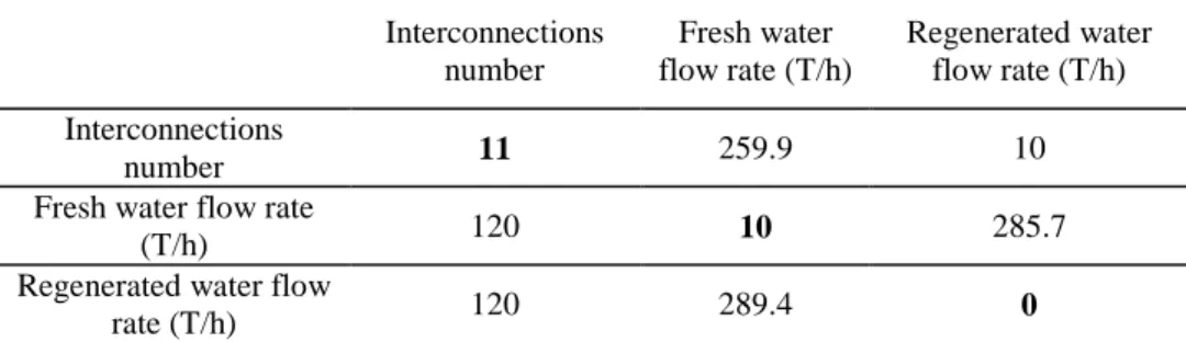
In order to set the problem limits, each objective was first minimized alone (see table 1), the minimum number of interconnections is 11, the minimum fresh water is 10 T.h-1, and the amount of regenerated water is null (all the used water is discharged, case without any practical interest). These values are reported in bold in table 1.

Table 1. Results of the mono-objective optimization

Interconnections number Fresh water flow rate (T/h) Regenerated water flow rate (T/h) Interconnections number 11 259.9 10

Fresh water flow rate

(T/h) 120 10 285.7

Regenerated water flow

rate (T/h) 120 289.4 0

Then, the biobjective optimization is performed for different values of the interconnection number. So, for 120 (respectively 11) interconnections, the Pareto fronts are reported in Fig. 1a (respectively 1b), Fig. 1c giving a zoom of Fig. 1b. Fig. 1d shows the minimum value of fresh water flow versus the number of interconnections (the regenerated water flow is not taken into account). As it was already shown in [3], the Pareto fronts of Fig. 1a, b and c are linear. For 120 interconnections, all the points located on the straight line are feasible solutions; for the minimum number of interconnections (11), the Pareto front is reduced and composed of a finite number of points located on a straight line with the same slope than the one corresponding to 120 interconnections. From Fig. 1b, no solution exists for a regeneration flow greater than 80 T.h-1. The results presented in Fig. 1c, obtained by taking a step length of 1 instead of 20 in the lexicographic procedure, shows no additional solution located between the points. From Fig. 1d, it can be observed that for 11, 12, 13 and 14 connections, the fresh water flow rate is respectively 90, 50, 25 and 10 T.h-1 and remains fixed at 10 T.h-1 when the number of interconnections varies from 15 up to 120.The values obtained for the example problem are identical with the ones reported in the literature [6, 9], so the solution procedure is numerically validated.

5.

Conclusion and future works

From this example, the following items can be pointed out: (i) for the maximum number of connections (120), the Pareto front is a straight line and all the points located on it are feasible solutions, (ii) the Pareto front is reduced with the number of connections, (iii) for low numbers of connections corresponding to highly constrained problems, the Pareto front is constituted by isolated points located on a straight line, and no feasible solution exists between the points. So the number of feasible solutions decreases with

M. Boix et al.

the number of connections. Finally, since it only requires a standard initialization phase and can tackle large scale problems, this approach will be implemented in the next future on the one hand to optimize ecopark networks, and on the other hand to solve multicontaminant problems.

Fig.1 Pareto fronts obtained with the biobjective optimizations

References

[1] B. Dave and O. Nalco., National Academy Press, (2002).

[2] Z.A Manan, S.R. Wan Alwi and Z. Ujang, Desalination, 194 (2006) 52.

[3] R.F. Dunn and M.M. El-Halwagi, J. Chem. Technol. Biotechnol., 78 (2003) 1011.

[4] J. Jacob, C. Viviant, H.F. Houle and J. Paris, Pulp Pap. Can., 103 (2002) 24.

[5] B. Linhoff and R. Smith, Pro. Sys. Eng., 1984.

[6] X. Feng, J. Bai, H. Wang and X. Zheng, Comput. Chem. Eng., 32 (2008) 1892.

[7] M. Savelski and M. Bagajewicz, Chem. Eng. Sci., 58 (2003) 5349.

[8] C.H. Huang, C.T. Chang and C.C. Chang, Ind. Eng. Chem. Res., 38 (1999) 2666. [9] M. Bagajewicz and M. Savelski, Chem. Eng. Res. Des. 79 (2001) 600.

[10] S. Shafiei, S. Domenech, R. Koteles and J. Paris, J. Clean. Prod., 12 (2003) 131. [11] N. Hallale and D.M. Fraser, Trans. Inst. Chem. Eng., 78 (2000) 202.

[12] M.M. El-Halwagi, Academic Press, CA, USA (1997).

[13] M.M. El-Halwagi, F. Gabriel and D. Harell, Proc. Des. Cont., 42 (2003) 4319. [14] Y.P. Wang and R. Smith, Chem. Eng. Sci., 49 (1994) 981.

[15] I. Quesada and I.E. Grossmann, Comp. Chem. Eng., 19 (1995) 1219. [16] B. Galan and I.E. Grossmann, Ind. Eng. Chem. Res., 37 (1998) 4036. [17] G. Mavrotas and D. Diakoulaki, Ap. Math. Comp., 171 (2005) 53.

a b

d c