HAL Id: hal-02623461
https://hal.inrae.fr/hal-02623461
Submitted on 26 May 2020
HAL is a multi-disciplinary open access archive for the deposit and dissemination of sci-entific research documents, whether they are pub-lished or not. The documents may come from teaching and research institutions in France or abroad, or from public or private research centers.
L’archive ouverte pluridisciplinaire HAL, est destinée au dépôt et à la diffusion de documents scientifiques de niveau recherche, publiés ou non, émanant des établissements d’enseignement et de recherche français ou étrangers, des laboratoires publics ou privés.
means of EthAcc
Brigitte Mangin, Renaud Rincent, Charles-Elie Rabier, Laurence Moreau,
Ellen Goudemand-Dugue
To cite this version:
Brigitte Mangin, Renaud Rincent, Charles-Elie Rabier, Laurence Moreau, Ellen Goudemand-Dugue. Training set optimization of genomic prediction by means of EthAcc. PLoS ONE, Public Library of Science, 2019, 14 (2), �10.1371/journal.pone.0205629�. �hal-02623461�
Training set optimization of genomic
prediction by means of EthAcc
Brigitte ManginID1*, Renaud Rincent2, Charles-Elie Rabier3,4, Laurence Moreau5, Ellen Goudemand-Dugue6
1 LIPM, Universite´ de Toulouse, INRA, CNRS, Castanet-Tolosan, France, 2 GDEC, INRA, Clermont-Ferrand, France, 3 ISEM, Univ. Montpellier, CNRS, EPHE, IRD, Montpellier, France, 4 LIRMM, Univ. Montpellier, CNRS, Montpellier, France, 5 GQE-Le Moulon, INRA, Univ Paris-Sud, CNRS, AgroParisTech, Universite´ Paris-Saclay, Gif-sur-Yvette, France, 6 LGB, Florimond Desprez Veuve & Fils, Cappelle-en-Pe´vèle, France
*brigitte.mangin@inra.fr
Abstract
Genomic prediction is a useful tool for plant and animal breeding programs and is starting to be used to predict human diseases as well. A shortcoming that slows down the genomic selection deployment is that the accuracy of the prediction is not known a priori. We propose EthAcc (Estimated THeoretical ACCuracy) as a method for estimating the accuracy given a training set that is genotyped and phenotyped. EthAcc is based on a causal quantitative trait loci model estimated by a genome-wide association study. This estimated causal model is crucial; therefore, we compared different methods to find the one yielding the best EthAcc. The multilocus mixed model was found to perform the best. We compared EthAcc to accu-racy estimators that can be derived via a mixed marker model. We showed that EthAcc is the only approach to correctly estimate the accuracy. Moreover, in case of a structured pop-ulation, in accordance with the achieved accuracy, EthAcc showed that the biggest training set is not always better than a smaller and closer training set. We then performed training set optimization with EthAcc and compared it to CDmean. EthAcc outperformed CDmean on real datasets from sugar beet, maize, and wheat. Nonetheless, its performance was mainly due to the use of an optimal but inaccessible set as a start of the optimization algo-rithm. EthAcc’s precision and algorithm issues prevent it from reaching a good training set with a random start. Despite this drawback, we demonstrated that a substantial gain in accu-racy can be obtained by performing training set optimization.
Introduction
Prediction of unobserved individuals using genomic information has gained increasing impor-tance in plant and animal breeding [1,2]. Moreover, it is an accurate tool for prediction of complex diseases in humans [3,4] and is included in the precision medicine initiative [5].
Basically, a training set of individuals, the so-called training set, that is both phenotyped and genotyped is used to train a model that is applied to predict unobserved individuals, the so-called test set, on the basis of only genotyping data from the latter. Many methods have
a1111111111 a1111111111 a1111111111 a1111111111 a1111111111 OPEN ACCESS
Citation: Mangin B, Rincent R, Rabier C-E, Moreau
L, Goudemand-Dugue E (2019) Training set optimization of genomic prediction by means of EthAcc. PLoS ONE 14(2): e0205629.https://doi. org/10.1371/journal.pone.0205629
Editor: Momiao Xiong, University of Texas School
of Public Health, UNITED STATES
Received: September 25, 2018 Accepted: January 3, 2019 Published: February 19, 2019
Copyright:© 2019 Mangin et al. This is an open access article distributed under the terms of the
Creative Commons Attribution License, which permits unrestricted use, distribution, and reproduction in any medium, provided the original author and source are credited.
Data Availability Statement: Maize data are
available at:http://www.genetics.org/lookup/suppl/
doi:10.1534/genetics.112.141473/-/DC1
Sugarbeet, Sunflower and wheat data are available at:https://lipm-browsers.toulouse.inra.fr/pub/ Mangin2018-PlosOne/.
Funding: BM, LM, EG-D have been supported by
the French National Research Agency (ANR:
https://www.agence-nationale-recherche.fr/) as part of the “Investissements d’Avenir” Program: AKER project ANR-11-BTBR-0007, AMAIZING project ANR-10-BTBR-03, and SUNRISE project
been proposed for the training model step that are included in the mixed model framework [6,7], in penalized regression methods [8], in Bayesian modeling [9], and in semiparametric and nonparametric learners [10,11]. These methods have been comprehensively compared, and depending on the trait under study, one or another method has been shown to be more reliable, but the best performers provide comparable accuracy rates [12,13]. In any case, geno-mic best linear unbiased prediction (GBLUP) [7] was shown to be competitive with more com-plicated models. Its ease of use and its efficient computer implementation explain its
development into a reference model. Moreover, the flexibility of the mixed model framework for modeling of nonadditive genetic factors or for incorporation of functional knowledge [14] explains the large number of extensions of the GBLUP model.
A shortcoming that slows down the genomic selection deployment is that the accuracy of the prediction is not known a priori and depends on a number of factors such as the size of the training set, trait architecture (especially its heritability), density of markers, relatedness between tests and trainings, and others. The prediction accuracy is useful for at least two pur-poses. One of them is to decide whether genomic selection is worth applying to a crop for a trait of interest. This accuracy is defined as the expectation of the prediction accuracy for a training set randomly drawn in a population. The second purpose is to allow for optimization of the training set used to predict the test individuals and must involve a quantity that enables discrimination among several training sets, and therefore it must be defined given a training set.
Most of the accuracy proxies have been developed for the first purpose, that is the expecta-tion of predicexpecta-tion accuracy for a random training set belonging to a populaexpecta-tion. Moreover, they have been developed by means of predictions obtained in a linear mixed model, known as GBLUP or equivalently ridge regression best linear unbiased prediction (RR-BLUP) because there is an analytical prediction of the genetic value in this case. Nonetheless, the first proxy proposed by Daetwyler et al. [15] was developed within a simpler model assuming that the genetic value is explained by a fixed number of independent quantitative trait loci (QTLs). This seminal formula was generalized later by Goddard [16] who linked accuracy to the effec-tive number of segments in the genome by adding the assumption that the QTL effects are independent and identically distributed. From these two papers, different formulas have been derived that linked the prediction accuracy to heritabilityh2, training population sizeT, the
number of markersM, and the number of effective segments in the genome Me[16–18]. Some
authors [19] compared these formulas with a meta-analysis of 13 papers in which prediction accuracy was computed using both simulated or real data. They showed that training popula-tion sizeT and the effective number of segments Mehave a significant impact on the accuracy;
this situation is cause for concern becauseMecan be estimated in several models that yield
very different values [20]. They also demonstrated that among the different formulas, none outperforms the others. Until recently, Goddard’s formula has continued to give rise to new works such as the improvement proposed in [21] for theMeparameter. Nevertheless, all these
accuracy proxies derived from Goddard’s approach are based on a number of statistical and mathematical approximations that were clearly explained in [22]. That paper highlighted the difficulties of finding a proxy that reflects correctly the diversity of situations of training popu-lation structures and linkage disequilibrium between markers and QTLs.
Another proxy came from Rabier et al. [20] who developed a theoretical formula of the accuracy conditional to a given training set. In contrast to Goddard, Rabier et al [20] did not assume the independence of the QTLs or a distribution of the QTL effects but attempted to derive their formula using a fixed number of known causal QTLs. The major drawback of this theoretical formula is that the QTL locations and effects have to be estimated first and plugged into the formula to get an estimate of the prediction accuracy, that we call “EthAcc” here
ANR-11-BTBR-0005. The Florimond Desprez Veuve & Fils company provided support in the form of a salary for D. The specific roles of EG-D are articulated in the ‘author contributions’ section. The funders had no role in study design, data collection and analysis, decision to publish, or preparation of the manuscript.
Competing interests: The Florimond Desprez
Veuve & Fils company provided support in the form of a salary for EG-D. This does not alter our adherence to PLOS ONE policies on sharing data and materials. There are no patents, products in development, or market products to declare.
(Estimated THeoretical ACCuracy). Contrary to the above proxies that are estimates of the expectation of prediction accuracy for a training set randomly drawn from a given population, EthAcc is an estimator of the genomic prediction accuracy of a given training set. It could then be used to optimize the training set to increase the accuracy by choosing the trainings that together performed the best on the test predictions.
Panel optimization for genomic prediction was first proposed by Rincent et al [23]. They supposed that a panel of candidates has been genotyped and that the goal is to choose the best set to phenotype (i.e., the training individuals). The same objective was later addressed by the authors of [24]. Both research groups proposed to perform panel optimization with a fixed size of the training set, which is consistent when assuming a limited budget proportional to candi-dates to be phenotyped (i.e., the training set). Moreover, the two criteria upon which they based the optimization generally increase with the training set size, and therefore a fixed size is necessary to obtain an optimized training set that is smaller than the whole panel of candidates. The question of training panel optimization for the test prediction is more suitable for geno-mic selection per se. In a breeding company, as an example, past breeding panels that have already been phenotyped are nowadays genotyped. They constitute the resources upon which genomic models can be trained. At the same time, new breeding resources are created and genotyped but are still not phenotyped. These resources have to be subjected to genomic selec-tion, and the key task is to choose the best training set from genotyped and phenotyped past resources to optimally predict the current resources.
Materials and methods
The genomic prediction of the genetic value of test individuals was based on GBLUP [7], and we define the accuracy of genomic prediction as Pearson’s correlation between its phenotype and its BLUP-value for a random test individual and a given training set. We refer to this cor-relation as the accuracy in the text below.
This accuracy is a theoretical quantity that is usually estimated using the mean of empirical Pearson’s correlation between phenotypic values and their GBLUP for a random test set. In statistics, this estimate is called an empirical estimate or sample estimate, but we call it the test set (TS) accuracy in the analysis that follows. This TS accuracy can be calculated only if pheno-types are observed in test individuals, which is the case when the TS is randomly drawn within a dataset or obtained by a simulation process. This TS accuracy was compared to three meth-ods that estimate the accuracy without making use of the test set phenotypic observations.
Accuracy estimated given a training set
The idea behind finding an estimate of the accuracy is to confound the causal-QTL model which emulates the genetic value with QTLs to the model used to make the prediction of the genetic value using markers. As we focus on the prediction obtained by GBLUP or equivalently by RR-BLUP, this confusion means that each marker is assumed to be a QTL, and the QTL effects are assumed to be independent and identically distributed according to a Gaussian dis-tribution. We called this confusion “the GBLUP model of the genetic value”. In the GBLUP model, the coefficient of determination (CD) of the genetic value of a test individual is by defi-nition the square correlation between the genetic value and its predictor. This accuracy is known to be linked to the accuracy involving the phenotypic value by the square root of herita-bility [25]; thus, the first accuracy estimate is
^ rCD¼ 1 ntest X i ffiffiffiffiffiffiffiffiffiffiffiffiffiffiffiffiffiffiffiffiffiffiffiffiffiffiffiffiffiffiffiffiffiffiffiffiffiffiffiffiffiffiffiffiffiffiffiffiffi Varðutest;iÞ Varðutest;iÞ þ s2ε CDðutest;iÞ s
whereutest,iis the random genetic value of theith individual in a TS, ntestis the number of test
individuals, and s2
εdenotes the residual variance using the GBLUP model.
The second method for predicting the accuracy is based on the prediction error variance (PEV) involving the GBLUP model. By definition, PEV is the variance of the difference between an individual genetic value and its predictor. In the GBLUP model, it can be proved that Covð^uBLUP
test;i;utest;iÞ ¼ Varð^uBLUPtest;iÞ and so PEVðutest;iÞ ¼ Varðutest;iÞ Covð^uBLUPtest;i ;utest;iÞ, where ^uBLUP
test;i is the BLUP predictor of theith individual. Therefore, the second accuracy esti-mate is ^ rPEV¼ 1 ntest X i ffiffiffiffiffiffiffiffiffiffiffiffiffiffiffiffiffiffiffiffiffiffiffiffiffiffiffiffiffiffiffiffiffiffiffiffiffiffiffiffiffiffiffiffiffiffiffiffiffiffiffiffiffiffiffiffiffiffiffiffiffiffiffiffiffiffiffi Varðutest;iÞ Varðutest;iÞ þ s2ε 1 PEVðutest;iÞ Varðutest;iÞ ! v u u t
Both CD and PEV rely on the GBLUP model, or equivalently the RR-BLUP model [26] that is presented here:
ytrain¼ 1m þXtrainβ þ ε
whereμ is the global mean, 1 represents a vector of 1, Xtrainis the matrix of SNP genotypes for
individuals in the training set, andytraindenotes their observed phenotypes.β is the vector
of SNP effects assumed to be independent and identically distributed (iid) with Gaussian dis-tributionN ð0; s2
bÞ, andε is the vector of residual errors assumed to be iid with Gaussian distributionN ð0; s2
εÞ, independent ofβ. Moreover, utest,iis assumed to be equal tox0test;iβ,
wherex0
test;iis the line vector of SNP genotypes for test individuali; accordingly, we get
Varðutest;iÞ ¼ s
2 bxtest;ix
0 test;i.
The third method is based on the work of [20] who theoretically derived the accuracy when QTL locations and effects are known. They developed their formula within a framework where the RR-BLUP model serves as an instrumental approach to getβ estimated values, whereas a linear causal model with a fixed number of known QTLs is assumed to model the phenotype as follows:
ytrain ¼ 1m þQtrainθ þ e
whereQtrainis the matrix of QTL genotypes for individuals in the training set,θ represents the
vector of QTL effects, ande denotes the vector of residual errors assumed to be iid with Gauss-ian distributionN ð0; s2
eÞ. Genetic valuegtest,iis assumed to be equal toq0test;iθ, where q
0 test;iis
the line vector of QTL genotypes for theith test individual.
Using the instrumental RR-BLUP model and the causal-QTL model, they obtained the fol-lowing theoretical formula of the accuracy for an individual randomly sampled in the test pop-ulation:
r ¼ θ
0
Eðqtest;ixtest;i 0ÞX0 trainH 1 Qtrainθ ðs2 eEðk xtest;iX 0 trainH 1 k2Þ þ θ0Q0 trainH 1
XtrainVarðxtest;iÞX 0 trainH 1 QtrainθÞ 1=2 ðs2 gþ s 2 eÞ 1=2
where k.k is theL2norm, s2
erepresents the error variance in the causal model, s
2 g¼ Varðgtest;iÞ andH ¼ XtrainX 0 trainþ s2 ε s2 bI � �
, withI denoting the identity matrix. Note that the formula is correct if matrices of SNP genotypes are previously column centered to make them orthogonal toμ.
To estimateρ, all quantities depending on a random individual in the test set are replaced
by the empirical or sample estimate (i.e., the mean across test individuals). s2
the least square method in the causal-QTL model by means of genotypes and phenotypes of training set individuals. Nevertheless, the location of QTLs and their effect have to be esti-mated if they are unknown.
For the three accuracy estimates, variance parameters s2
εand s2bare estimated by restricted maximum likelihood (REML) using genotypic and phenotypic data of training set individuals.
Estimation of a causal-QTL model
The authors of [27] used penalized regression methods to detect the QTLs and to estimate their effects though it is well known that penalized regression yields biased estimators of QTL effects. In this paper, we used a two-step procedure, the first step was to locate the QTLs via multi-QTL methods developed for a genome-wide association study (GWAS), then the QTL effects were estimated via a classical linear model by the ordinary least square method as well as the error variance in the causal model s2
e.
One of multi-QTL methods is the forward selection approach of the multilocus mixed model (MLMM) proposed in [28]. A classical marker-by-marker GWAS model [29] with a VanRaden’s kinship matrix [7] for the polygenic effect and no fixed structure effect is employed. The forward selection approach is an iterative technique, where at each step, the SNP with the minimum p-value is added into the model as a fixed effect, and a rescan of the remaining SNPs is performed. The iterative procedure stops when the variance of the poly-genic effect is close to zero, meaning that the discovered SNPs that have been added into the model as fixed effects together explain almost all the polygenic variability. This final model outputs the discovered SNPs as causal QTLs.
The others multi-QTL methods used penalized regressions. They were thoroughly com-pared for GWAS by Waldman et al. [30]. Consequently, we based our choices for penalization parameters of the least absolute shrinkage and selection operator (LASSO) and the elastic net (EN) upon their comparisons. We computed LASSO shrinkage parametersλ by a 10-fold cross-validation schema, and we calculated the optimalλ from the minimum mean square error (minMSE) of the predictor and minMSE plus one standard error (1SE) of minMSE. Recently, Yi et al. [31] proposed a false discovery rate (FDR) control to make the choice of the λ parameter. We chose the analytical FDR control because it has been shown to perform the best on SNP selection [31]. The ENα parameter was set to 0.5 and 0.1. To complete the penal-ized regression methods, we added the adaptive LASSO [32] that gives the most accurate results when QTL effects are estimated by penalized regression estimators [27].
Once causal QTLs were located, their effects were all together estimated by the ordinary least square method via a classical linear model, as well as the error variance of this estimated causal-QTL model. The ordinary least square method was applicable because we limited the number of QTLs searched in function of the number of individuals. Nevertheless, in practice, this constraint on the number of QTLs has never been applied.
Panel optimization
Panel optimization consists of choosing (within a panel of candidates) the set of training indi-viduals that better predicts a test belonging to a population of tests. One research group [23] proposed to use the CDmean criterion to make the choice. Later, [24] suggested to perform the optimization on the basis of PEV. CDmean is the mean acrossntesttest individualsi (i.e.,
sample estimate) of the CD for contrast between individual genetic valueutest,iand the
popula-tion mean (test + training individuals). The criterion on the basis of PEV is the mean across
ntesttest individualsi (i.e., sample estimeate) of PEV of individual genetic value utest,i. CDmean
slightly better than PEV on panel optimization [23] even for a mildly structured population [33,34].
The panel optimization burden was dealt with by the hill-climbing algorithm with exchange moves that was proposed in [23]. We did not implement a stopping criterion to always per-form a given number of exchange moves. The number of exchange moves was set to 5000.
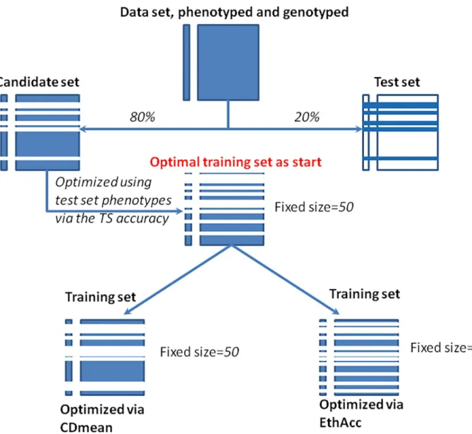
The starting training set of the hill-climbing algorithm for both criteria was the optimal training set found by maximization of the TS accuracy, i.e., we found the training set that gave a maximum for the mean correlation between GBLUP and the observed phenotypes of the test individuals. This maximization of the TS accuracy was possible because the TS was randomly drawn within the whole dataset, and therefore test individuals had phenotypes. Having this set as a start of the algorithm prevents it from getting stuck in a local maximum that is far from the maximum of the TS accuracy. Starting with this optimal training set, we were able to mea-sure how the different criteria will degrade the maximum of the TS accuracy, in other words, how big the decrease in accuracy (caused by each criterion) will be.
Fig 1resumes the optimization process for a random sampling of the test set. For CDmean calculation, the variance components of the RR-BLUP model, s2
εand s2b, were estimated by REML with the entire candidate panel to obtain the most precise estimated val-ues. The causal-QTL model of EthAcc was discovered by the forward selection approach of MLMM applied to the current training set. It was thus re-evaluated at each new training set.
At the end of the optimization burden, the TS accuracy was computed via the RR-BLUP model trained on the respective optimal training set of each criterion.
Simulation implementations
Method comparisons were made by randomly drawing a TS within the whole panel. Unless precise, 20% of the panel served as a TS and the remaining individuals were the candidates or the largest training set when we did not perform training set optimization. To ensure accurate comparisons, the TS accuracy and the accuracy estimates were computed on the same TS. The results were obtained for 30 random TS draws.
Predicted genetic values of TS individuals were obtained by estimating SNP effects with the training set by means of the mixed.solve function of R package rrBLUPhttps://cran.r-project. org/web/packages/rrBLUP/index.html. This function was also applied to compute CD, PEV, and CDmean via our own R code.
The R code for computing EthAcc (from a training set that is genotyped and phenotyped and a test set that is only genotyped) is given inS1 File. We used our own R code, which was rewritten based on Segura’s code [28] and that is now available on CRAN https://cran.r-project.org/web/packages/mlmm.gwas/index.html, to implement the forward selection MLMM approach. The glmnet R packagehttps://cran.r-project.org/web/packages/glmnet/ index.htmlwas used to perform localization of QTLs by penalized regression methods. The parcor R packagehttps://cran.r-project.org/web/packages/parcor/index.htmlwith the parame-ter of cross-validation set to 5 was used to perform adaptive LASSO.
To avoid computation issues, SNP filtration on minor allele frequency (MAF) was carried out. All code can be provided on request.
Plant material
Maize data has been downloaded fromhttp://www.genetics.org/content/suppl/2012/08/03/ genetics.112.141473.DC1. Sugar beet, sunflower and wheat data are available at https://lipm-browsers.toulouse.inra.fr/pub/Mangin2018-PlosOne/
Sugar beet. A panel of 2101 elite lines of diploid sugar beet (Beta vulgaris L.), which
resulted from many different crosses in Florimond Desprez’s breeding program, was analyzed. Testcross progenies of these lines were evaluated in unbalanced multienvironment trials for seven traits: the white sugar yield (WSY, t/ha), sugar content (S, %), white sugar content (WS, %), the root yield (RY, t/ha), potassium content (K, meq/100 g), sodium content (Na, meq/100 g), andα-amino nitrogen content (N, meq/100 g). The sugar beet panel was finger-printed with 836 SNP markers, but the panel was analyzed with 692 SNPs after filtration for MAF and missing data (see details inS1 File). The structure of subpopulations in this panel was then studied. We applied hierarchical clustering to principal components using the Facto-MineR packagehttps://cran.r-project.org/web/packages/FactoMineR/index.html[35] in R software to assign each individual to a subpopulation after principal component analysis (PCA). The HCPC function of the FactoMineR package implements this calculation after hav-ing constructed the hierarchy and suggests an optimal level for division.
Fig 1. Illustration of the sampling and of the optimization process that were implemented to compare CDmean and EthAcc criteria.
Sunflower. Sunflower data covered hybrids obtained by crossing 36 restorer of CMS PET1 male sterility lines serving as males to 36 maintainer lines as females in an incomplete factorial as described elsewhere [36]. Hybrid genotyping data were obtained from the whole-genome sequencing of their parents. A total of 468 194 nonredundant SNPs passed the differ-ent filters [36] and were used to compute their kinships. The phenotype trait, adjusted for field effects [36], was oil content in the 13EX01 environment with nonmissing data on 272 hybrids.
The test set was compiled by randomly sampling seven parents among the 72 parents (roughly 10%), and we placed all their descendants in the test set. This sampling produced a test set consisting of only T1 or T0 hybrids, as described by authors in [37], which have been shown to be difficult to predict because they are more distant from the possible training sets [36].
Maize. The two maize diversity panels employed in this study are some lines of the Flint and Dent panels that passed the genotyping and phenotyping filters described in [23]. Each panel is composed of 261 lines, genotyped for 30 027 and 29 094 markers for the Dent and the Flint lines, respectively, and crossed to a tester belonging to the other panel for hybrid pheno-typing. Two traits were analyzed: the mean of male flowering time (Tass_GDD6) and the plant dry matter yield (DM_Yield) that were observed in 2010 at four or five locations in Europe.
Wheat. A sample of 296 bread wheat accessions was employed for this study. This sample is a part of the INRA bread wheat core collection of 372 accessions (372CC) set up by [38]. Each accession was genotyped for 2013 markers (SSR, DArT, and SNP) covering the whole genome [39,40]. The SSR markers were transformed into biallelic markers by considering the different alleles independently. Each accession was phenotyped for heading date (day of year, DOY) in Clermont-Ferrand (France) in 2005. For this purpose, 10 seeds of each accession were sown in a single row on 27 October 2004. Ear emergence day of the main tiller of five to six individual plants was recorded when half of the ear had emerged from the flag leaf. The numbers were averaged to obtain the heading date for each accession [40].
Results
EthAcc as an accurate estimate of the accuracy
The theoretical accuracy formula proposed by Rabier et al [20] was shown by simulation to be an accurate predictor of the accuracy when causal-QTLs are known. Nevertheless, the QTL estimation step may have destroyed this desirable property. Thus, we studied the ability of EthAcc to predict the accuracy.
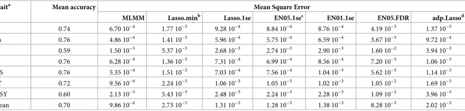
How to estimate the causal QTLs for EthAcc?. The question of the best choice of the QTL detection methods necessary for EthAcc computation was addressed first. Method com-parisons were made by randomly drawing a TS within the whole sugar beet panel. The mean accuracy and mean square error (MSE) as compared to the TS accuracy, were computed based on 100 random TSs for each trait. All traits were well predicted with the mean accuracy rang-ing from 0.59 forα-amino nitrogen content (N) to 0.76 for sugar content (S), white sugar con-tent (WS), and sodium concon-tent (Na). The most important trait for breeding, the white sugar yield (WSY), was predicted with the accuracy 0.60 (Table 1). Results clearly highlighted MLMM forward selection as the best choice for locating causal QTLs to be plugged into EthAcc. Whatever the trait that was considered, the MLMM QTL search outperformed all the other methods tested (lowest MSE). The influence of the criterion used to choose the LASSO shrinkage parameter seems to be the most important factor in the ranking of penalized regres-sion methods. After the best performer (MLMM), the penalized regresregres-sion methods are classi-fied by, first, the criterion of minimum MSE plus one standard error (Lasso.1se, EN05.1se, EN01.1se), then the minimum MSE criterion (Lasso.min), and finally the FDR criterion
(EN05.FDR). The adaptive LASSO was ranked between penalized regresions using the best cri-terion (.1se) and the second one (.min). For the WSY trait (which is one of the most difficult traits to predict) having the accuracy of 0.60 on average, the MLMM method reached the low-est MSE (2.13 10−3), whereas the EN05.FDR method was fivefold worse, with the highest MSE (1.09 10−2).
EthAcc behavior shows that “bigger is not always better”. The structure of the sugar beet panel was analyzed to assess the influence of population structure on the accuracy of pre-diction. The optimal cluster number of the hierarchical clustering in PCA [35] was set to 2. Sugar beet lines were represented in the first two principal components (see Fig A inS1 File). Clusters contained respectively 676 (Panel_A) and 1425 lines (Panel_B).
We addressed the question of whether it is better to train a model within a cluster or by means of the two clusters for prediction of a TS belonging to a unique cluster. We also com-pared EthAcc to the two other estimators of the accuracy: CD and PEV. TSs were randomly drawn specifically in a unique cluster (20% of the cluster size), and the model was trained either with all the remaining individuals of this cluster or with the remaining individuals of the whole panel (i.e., both clusters). Results on the mean accuracy among 100 randomly drawn TSs together with EthAcc, CD, and PEV means for each trait are presented inTable 2. When the TS belonged to Panel_A, it was better to include in the training set only the remaining indi-viduals of Panel_A (i.e., 540 indiindi-viduals) rather than adding all indiindi-viduals of Panel_B (i.e., 1425 individuals). Indeed, whatever the trait analyzed, the mean accuracy was higher when both trainings and tests belonged to the same cluster, even if training sets were smaller (540 vs 1965 individuals). The increase in accuracy reached 14% (α-amino nitrogen content) and was of 5% on average among all the traits, while the training set was more than threefold smaller. Opposite results were obtained in the other cluster (Panel_B). In this case, the mean accuracy was always higher when all the remaining individuals from both clusters were used. The increase in the training set size (1140 vs 1816 individuals) led to an 8% increase in the accuracy on average among all the traits. The largest increase, 19%, was obtained for WSY with the mean accuracy of 0.640 when the training set was composed of individuals belonging to both
Table 1. The accuracy and MSE of EthAcc compared to the TS accuracy according to several methods for estimation of causal QTLs on different traits (mean over 100 random test-training sets).
Traita Mean accuracy Mean Square Error
MLMM Lasso.minb Lasso.1se EN05.1sec EN01.1se EN05.FDR adp.Lassod
K 0.74 6.70 10−4 1.77 10−3 9.28 10−4 8.84 10−4 8.76 10−4 4.19 10−3 1.37 10−3 Na 0.76 4.86 10−4 1.41 10−3 5.96 10−4 5.75 10−4 6.59 10−4 3.67 10−3 9.72 10−4 N 0.59 1.50 10−3 5.37 10−3 2.68 10−3 2.74 10−3 2.90 10−3 1.60 10−2 3.94 10−3 S 0.76 6.28 10−4 1.36 10−3 7.31 10−4 6.99 10−4 8.56 10−4 7.20 10−3 1.06 10−3 WS 0.76 5.35 10−4 1.51 10−3 7.03 10−4 7.56 10−4 1.04 10−3 5.62 10−3 1.14 10−3 RY 0.72 9.56 10−4 2.24 10−3 1.06 10−3 1.05 10−3 1.02 10−3 1.05 10−2 1.69 10−3 WSY 0.60 2.13 10−3 5.43 10−3 2.48 10−3 2.24 10−3 2.28 10−3 1.09 10−2 3.96 10−3 Mean 0.70 9.86 10−4 2.73 10−3 1.31 10−3 1.28 10−3 1.38 10−3 8.28 10−3 2.02 10−3
apotassium content in meq/100 g (K), sodium content in meq/100 g (Na),α-amino nitrogen content in meq/100 g (N), sugar content in % (S), white sugar content in %
(WS), the root yield in t/ha (RY), and the white sugar yield in t/ha (WSY)
b.min, .1se, and .FDR: choice of the LASSO shrinkage parametersλ based on the minimum MSE of the predictor (minMSE), minMSE plus one standard error (1SE) of
minMSE and FDR, respectively
cENx: EN with itsα parameter equal to x, dadp.Lasso: adaptive LASSO,
clusters, whereas the mean accuracy was only of 0.536 when the training set was composed only of individuals belonging to Panel_B.
The comparison of the three estimators of the accuracy highlighted the correct behavior of EthAcc and showed that both CD and PEV are not accurate. The mean accuracy was correctly estimated by EthAcc, whereas CD and PEV were very close and generally overestimated the mean accuracy. Contrary to CD and PEV, EthAcc was the only estimator showing that the big-ger training set was not always better for all the traits; this result was consistent with the mean accuracy. We performed a mean test comparison of the three estimators for their ability to evaluate the TS accuracy via the standard error correction proposed by [41] to take into account the dependencies of the sampled TSs (see the standard error correction and the test p-values in Table A inS1 File). Accuracy values estimated by CD and PEV were found to be significantly different (5% error risk) from the TS accuracy for all the traits and all the
test-Table 2. The accuracy and its values estimated by EthAcc, CD, and PEV using sugar beet structures in two clusters (Panel_A and Panel_B) on several traits (the mean for 100 random test sets).
Traita Test setb Training setb Mean accuracy Estimated by
EthAcc CD PEV K Panel_A Panel_A+B 0.712 0.696 0.818 0.818 K Panel_A Panel_A 0.742 0.734 0.823 0.824 Na Panel_A Panel_A+B 0.660 0.675 0.815 0.815 Na Panel_A Panel_A 0.689 0.676 0.776 0.777 N Panel_A Panel_A+B 0.500 0.552 0.744 0.745 N Panel_A Panel_A 0.571 0.588 0.678 0.680 S Panel_A Panel_A+B 0.665 0.684 0.851 0.851 S Panel_A Panel_A 0.682 0.690 0.801 0.802 WS Panel_A Panel_A+B 0.680 0.691 0.851 0.851 WS Panel_A Panel_A 0.700 0.698 0.809 0.810 RY Panel_A Panel_A+B 0.654 0.655 0.826 0.827 RY Panel_A Panel_A 0.688 0.699 0.790 0.792
WSY Panel_A Panel_A+B 0.583 0.562 0.735 0.735
WSY Panel_A Panel_A 0.597 0.603 0.702 0.703
K Panel_B Panel_A+B 0.752 0.780 0.887 0.888 K Panel_B Panel_B 0.714 0.715 0.788 0.789 Na Panel_B Panel_A+B 0.802 0.814 0.895 0.895 Na Panel_B Panel_B 0.773 0.769 0.814 0.815 N Panel_B Panel_A+B 0.637 0.669 0.869 0.869 N Panel_B Panel_B 0.567 0.560 0.733 0.734 S Panel_B Panel_A+B 0.800 0.813 0.899 0.900 S Panel_B Panel_B 0.759 0.757 0.817 0.818 WS Panel_B Panel_A+B 0.798 0.813 0.902 0.903 WS Panel_B Panel_B 0.759 0.754 0.820 0.822 RY Panel_B Panel_A+B 0.750 0.779 0.887 0.888 RY Panel_B Panel_B 0.703 0.696 0.783 0.785
WSY Panel_B Panel_A+B 0.640 0.644 0.865 0.865
WSY Panel_B Panel_B 0.536 0.527 0.678 0.680
apotassium content in meq/100 g (K), sodium content in meq/100 g (Na),α-amino nitrogen content in meq/100 g (N), sugar content in % (S), white sugar content in %
(WS), the root yield in t/ha (RY), and the white sugar yield in t/ha (WSY)
bcluster(s) to which the individual belongs https://doi.org/10.1371/journal.pone.0205629.t002
training panels (min p-value of 10−21, max p-value of 4 10−2), whereas the accuracy estimated by EthAcc was never deemed significantly different (min p-value of 6 10−2, max p-value of 0.99). The worse case for EthAcc, i.e., where EthAcc and the TS accuracy showed the largest difference, involved the root yield (RY) trait, a test set in Panel_B, and a training set belonging to both clusters. Nonetheless, on average among all the traits and all the test-training configu-rations, the accuracy estimated by EthAcc and that obtained on average seemed very close (mean p-value of 0.64).
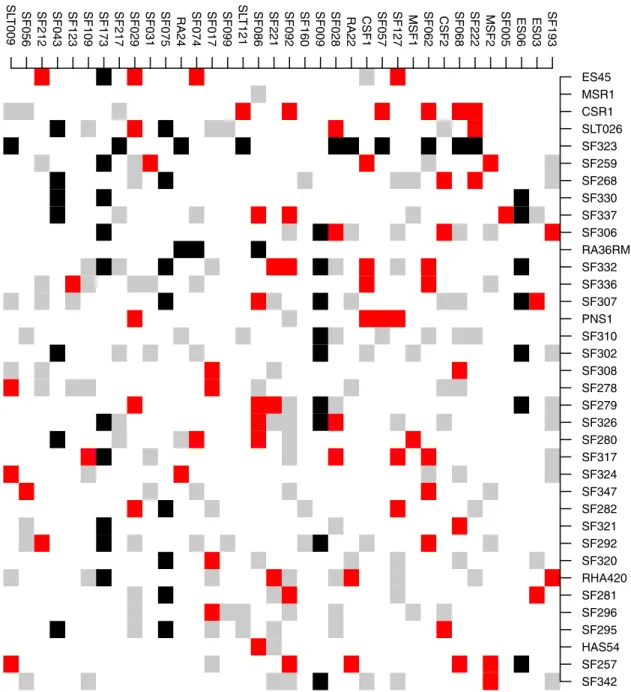
We showed that on average, the biggest training set is not always the best to make a predic-tion in a structured populapredic-tion. This conclusion is also valid for a test set in a nonstructured population, as is the case for the sunflower hybrid population.Fig 2presents a test set of T1 or T0 hybrids having a training set of 77 hybrids that yielded a TS accuracy of 0.745, whereas the TS accuracy with all the 218 hybrids as trainings is 0.722. This is not a great difference, but it indicates that in a particularly homogenous population that has not evolved, a training set adapted to the tests to be predicted can perform better than a bigger panel.
Comparison of EthAcc and CDmean for training set optimization
Fig 3depicts the comparison of the accuracy for optimization based on EthAcc with that based on CDmean. It is worth remembering that what is shown in this figure is the degradation pro-duced by CDmean and EthAcc of the maximum of the TS accuracy because the starting point of the hill-climbing algorithm for the two criteria is the training set giving the maximum of the TS accuracy. In all the cases, EthAcc yielded a smaller decrease in prediction accuracy than CDmean did. This result is expected because EthAcc estimates the accuracy via a model with a fixed number of QTLs whereas CDmean estimates the accuracy by means of a model with as many QTLs as markers, moreover assuming that QTL effects are Gaussian distributed.
Toward an understanding of differences between EthAcc and CDmean
To illustrate the difference in optimized training sets when we optimized the trainings using EthAcc or CDmean, we chose the test set that manifested the biggest difference in the TS accu-racy values. This test set involved the Flint panel for the DM_Yield trait and a fixed training set size of 50 individuals. Its TS accuracy was 0.07 and 0.76 when CDmean or EthAcc, respec-tively, served as the optimization criterion.Fig 4depicts these optimized training sets in a net-work representation. The kinship matrix that was employed to build the (0-1) netnet-work was VanRanden’s kinship matrix subject to a threshold equal to 0.77 (i.e., individuals were linked in the network if their kinship was greater than 0.77).
Results shown inFig 4clearly indicate that the optimization with the EthAcc criterion on the one hand and CDmean criterion on the other hand did not select the same individuals into their training sets to predict the same test set. This difference in selection can explain the extreme difference in the accuracy that was observed with the two training sets. Only 11 indi-viduals out of 50 were identical between EthAcc and CDmean, represented by yellow circles in
Fig 4. CDmean chose mostly individuals in the training set that are directly or indirectly linked in the network to individuals in the test set (i.e., kinship coefficient > 0.77). Only three indi-viduals that were less related to the test set were selected. In contrast, EthAcc selected fewer individuals with high kinship coefficients toward test set individuals. Indeed, 18 out of 50 indi-viduals belonging to the training set were unlinked in the network to the indiindi-viduals of the test set. To delve deeper into what happened, we compared the causal QTLs detected by the for-ward selection approach of MLMM in the two training sets previously optimized by CDmean and EthAcc. Eight and five SNPs were detected with the EthAcc and CDmean training sets, respectively. Among the eight SNPs detected in the EthAcc training set, a single SNP was rare
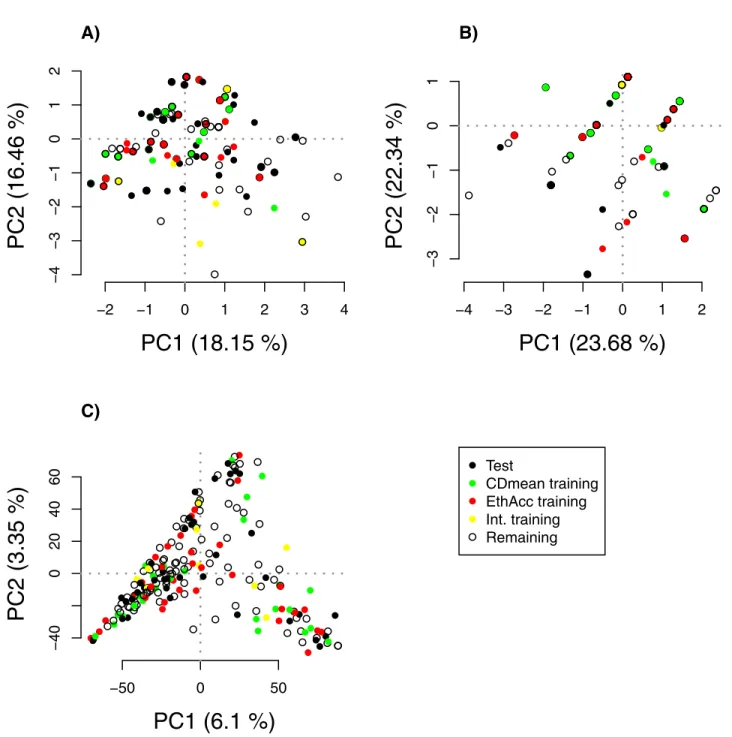
in the training set (MAF lower than 10% in the training set), whereas three out of five of the SNPs detected in the CDmean were rare (see Tables B and C inS1 File). The reduction in training set diversity caused by the CDmean criterion resulted in GWAS signals for rare SNPs and a prediction with the highest weights on those rare SNPs and on their linked SNPs. To confirm this observation, PCA was conducted with the detected SNPs and with all the SNPs for comparison. All individuals (test, training, and the remaining individuals) were projected onto the first two principal components (Fig 5), but test individuals were not used in the
Fig 2. SUNRISE hybrids obtained from 36 maintainer lines (females, rows) crossed to 36 restorer lines (males, columns).
Parental lines are arranged according to the hierarchical clustering based on VanRaden’s kinship matrices. Black squares indicate the 54 T0 or T1 hybrids in the test set, red squares are the 77 training individuals, and grey squares are hybrids that were among candidates but were not chosen to be in the training set.
analysis to construct components. We can see that the detected SNPs of the CDmean training set clearly structured the panel by reducing diversity with relatedness, in contrast to the detected SNPs of the EthAcc training set, which did not emphasize any structure.
Issues with training set optimization via EthAcc
Even though EthAcc performs quite well when the starting set of optimization is the optimal training set, we had to face numerical and algorithmic problems when performing optimiza-tion with a random training set as start.
One of these problems was due to what seems to be overparametrization of the step of learning causal QTLs. The causal QTLs were learned with MLMM for each new training set, and some false positive training sets were always produced by the optimization process (i.e., a training set with a high EthAcc value, close to 1, but low TS accuracy). We found a solution to this problem. Indeed, we observed that all false positive training sets yielded a high variance of the TS predicted genetic values. Because this variance is evaluated in the estimated causal-QTL
Fig 3. A significant increase in the TS accuracy produced by training set optimization with EthAcc compared to CDmean for several training set sizes and different datasets. The optimal (but inaccessible without test phenotypes) training set is the starting set of the optimization process. The black boxplot corresponds to the largest
training set. A) WSY within sugar beet Panel_A. B) DOY for wheat. C) DM_Yield within the Dent panel. D) DM_Yield within the Flint panel. E) Tass_GDD6 within the Dent panel. E) Tass_GDD6 within the Flint panel. Boxplots were constructed from 30 random test sets representing 20% of the whole panel.
model, it seems that for a given test set, we can always find a training set that produces high dispersion of the TS genetic values. A solution was then to reduce the original phenotype to a variance of one and to prevent EthAcc from reaching these training sets by means of a con-straint on this TS genetic value variance (by requiring that it is strictly less than 1). In other words, we forbided EthAcc from estimating a genetic variance greater than the phenotypic variance.
The second problem is an algorithmic problem, as illustrated inFig 6. This is a plot of the EthAcc values of training sets computed during the hill-climbing algorithm with 20 000 moves. The same TS was chosen for the optimization process with five random training sets and the optimal one, as starting sets. The hill-climbing moves are represented by red circles and the other moves (except those that are discarded due to the constraint) are plotted as grey triangles. It is clear that despite five random starts, each with 20 000 moves, the maximum value of EthAcc is not yet reached. Finding the training set that maximizes EthAcc is a
Fig 4. Network representation to highlight the differences in optimized training sets obtained with EthAcc and CDmean as optimization criteria. The data involve a test set of the Flint panel for the DM_Yield trait. This test set
had the accuracy of 0.07 and 0.76 when we used as training sets those optimized by CDmean and EthAcc, respectively. The network representation is based on VanRanden’s kinship matrix containing 25 682 SNPs subject to a threshold equal to 0.77 (i.e., individuals were linked in the network if their kinship coefficient was greater than 0.77). Individuals belonging to the test set, the training set optimized via EthAcc, the training set optimized via CDmean, the intersection of the two training sets, and the remaining set are black, red, green, yellow, and white circles, respectively.
Fig 5. The first principal component plane based on SNP markers: A) SNPs detected by the MLMM forward selection approach in the training set
optimized by EthAcc, B) SNPs detected by the MLMM forward selection approach in the training set optimized by CDmean, C) all SNPs with MAF greater than 0.05. Test set individuals were projected onto the plane but were not included in the computation of PCA axes. The test set is from the Flint panel for the DM_Yield trait. This test set had the accuracy of 0.07 and 0.76 when we used as training sets those optimized via CDmean and EthAcc, respectively. Individuals belonging to the test set, the training set optimized via EthAcc, the training set optimized via CDmean, the intersection of the two training sets, and the remaining set are plotted as black, red, green, yellow, and white circles, respectively.
combinatorial optimization that is really difficult to solve due to the causal-QTL learning step. Other algorithms could have been tested [42]; however, the results would have been almost the same because the optimal training set seems to be very specific.
Moreover, the precision of EthAcc is variable: even though we obtained an average mean square error close to 10−3, some training sets yielded an absolute difference between EthAcc and the TS accuracy greater than 0.5. Such a huge difference, due to the QTL estimation step
Fig 6. Hill-climbing moves for the optimal (but inaccessible without test phenotypes) training set (first column) and five random training sets serving as starts. Red circles denote the training sets that produced an increase of the current EthAcc value, and grey triangles represent the training sets
that did not increase the current EthAcc value. A total of 20 000 moves represented each start.
and the simple linear QTL model of the phenotype, prevents the algorithm from reaching obviously desirable training sets: those with both a high EthAcc value and TS accuracy.
Discussion
We have compared several estimates to infer the accuracy of GBLUP for a given training set (i.e., Pearson’s correlation between the observed phenotype and the predicted genetic value of tests given a training set genotyping). We demonstrated that neither CD- nor PEV-based accu-racy estimators are accurate. The reason is that both implied that the causal-QTL model, which emulates the genetic value, is identical to the linear mixed marker model that enables making the prediction. This model equality implies that each marker is a QTL and that the QTL effects are independent and identically distributed according to a Gaussian distribution. These assumptions on QTL effects (and thus on the genetic value) are asymptotically correct in the pedigree mixed model because it is proved to be the consequence of random draws of individuals in a lineage and an infinite number of equal and additive loci [43]. On the other hand, to estimate the accuracy precisely, the essential missing information is the identical-by-descent status of alleles at the causal loci between the test and the training individuals. This missing information has to be reflected by the marker-based kinship matrix, and a lot of research has been published regarding improvement of this kinship estimation [14,44,45]. In contrast to this way of thinking stuck in the mixed model framework, Rabier et al. [20] pro-posed an estimate of the accuracy by working in an instrumental mixed marker model to pre-dict the genetic value and a causal fixed linear model to emulate the genetic values. Into their theoretical accuracy formula, we plugged the location and the SNP effect estimated by the for-ward MLMM approach [28]. Thus, we showed on real data that we obtained an accurate esti-mate of the accuracy (MSE of 10−3on average among sugar beet traits).
Having an estimate of the accuracy for a given training set requires knowledge of the geno-typing of the training set but allows researchers to easily obtain an estimate of the expectation of the accuracy for a training set randomly drawn in a population. Indeed, this accuracy expec-tation can be calculated by performing random draws of training sets and taking the mean. This accuracy expectation was the goal of the different formulas derived from the works of [15,
16]. Via estimation of the QTL locations and effects, the authors of [27] compared the expecta-tion of the theoretical accuracy to these analytical formulas and found that the former per-formed better than the other formulas. The most important issue with the theoretical accuracy formula is the estimation of the causal-QTL locations and effects. The authors of [27] com-pared different penalized regression methods and revealed that adaptive LASSO [32] per-formed the best. We also compared different methods by plugging them into the theoretical accuracy formula, but in contrast to [27], we did not use the penalized regression estimators of the QTL effects because they are known to be biased. We used a two-step procedure to avoid this bias, whereas MLMM and penalized regression methods were employed to locate the QTLs, and their effects were estimated by classical ordinary least square methods. We based our choice to locate the QTLs on the comparison implemented by [30] for GWAS, and we added the analytical FDR control because it has been shown to perform the best on SNP selec-tion [31], MLMM [28] and adaptive LASSO [32]. We ranked EN (except with the FDR con-trol) before LASSO in terms of mean squared error as compared to the TS accuracy. Adaptive LASSO was ranked after penalized regressions that based their choice for the LASSO skrinkage parameter on the criterion of minimum MSE plus one standard error; however, MLMM was the best performer.
Accordingly, the theoretical accuracy with QTL locations obtained by MLMM was named EthAcc for Estimated THeoretical ACCuracy. We proposed R code to compute EthAcc that
does not involve Henderson’s mixed model equations, as opposed to [23] and [33], but made all the calculations based on the ridge regression matrixH ¼ XtrainX
0 trainþ s2 ε s2 bI � � , whereXtrain
is a matrix of genomic information of training individuals. The reason is the necessity to have an invertible kinship matrix to use Henderson’s equations, which is not the case for VanRa-den’s kinship matrix. When not invertible, the kinship matrix is generally projected on the cone of positive–definite matrices which create computation approximations. Moreover, Hen-derson’s equations are effective when the size of recorded data is huge as compared to the training set size, which is generally the case in animal breeding evaluation as the data are recorded on females while the males are evaluated. By contrast, in plant breeding, there is gen-erally one record per individual on evaluation; therefore, it is simple and more effective to use ridge regression matrixH. Nevertheless, EthAcc can also be computed via Henderson’s equa-tions; this approach makes sense when the kinship matrix is not a marker-based matrix.
EthAcc allows us to perform optimization of training individuals to predict and we com-pared it to training set optimization with CDmean [23]. EthAcc clearly outperformed CDmean on all the real data we tested (sugar beet, maize, and wheat). Nonetheless, this performance was due to the fact that we started the optimization burden with the optimal training set by means of the test set phenotypes to find it. Close to this optimal training set, EthAcc finds a good training set (because it is an accurate estimate of the accuracy), whereas CDmean chose a training set that strongly decreases the maximum of the TS accuracy by increasing the related-ness of individuals. In contrast, with a random training set as start, algorithmic and precision issues prevent EthAcc from reaching good training sets and despite a lot of attempts we did not succeed in making EthAcc perform correct training set optimization. Certainly, we could have performed optimization with a more effective algorithm than the hill-climbing algorithm or we could have increased the number of hill-climbing moves. MLMM is a long CPU software application, especially with a high number of markers but it could be replaced by the best penalized regression which is much faster and therefore allows much more moves. Neverthe-less, the crucial point is the precision of EthAcc. Indeed, a MSE of 10−3on average is not a guarantee of having a close estimate of the accuracy. During the optimization process, some training sets were mostly overestimated then yielding false positive training sets. The precision of the theoretical accuracy—with known causal-QTL locations and effects—was shown to be much higher [20,27]. This finding suggests that the QTL localization should be improved. Adding functional information such as candidate genes, metabolic networks, and transcription factors may help to explore various ways to facilitate the QTL localization by limiting the search to fragments of the genome that are known to be involved in the trait of interest. Nevertheless, the task of funding causal genome fragments is daunting, and if there are too many missing causal regions, a decrease in accuracy can be observed, as in sunflower hybrids when the oil metabolic network is used to predict oil content [36]. EthAcc is derived from a linear additive causal-QTL model. This simple model can be made more real by model-ing the interaction between causal QTLs. A more generalized theoretical formula has to be devised in such a model, but the procedure developed in [20] can be applied without any difficulty.
Despite the drawbacks of EthAcc, we illustrated that a substantial gain in accuracy can be obtained by performing training set optimization (up to 100% in the Flint maize panel with a yield). This accomplishment is quite different from the small differences among all the pub-lished methods for improving prediction (i.e., linear mixed models, penalized regression anal-yses, Bayesian methods, and nonparametric models). Such an increase in accuracy is worth the time spent on work on training set optimization, in particular with a complex and highly
polymorphic trait. Moreover, we showed that increasing the training population size does not always lead to better performance relative to optimization of the training set.
Supporting information
S1 File. Content. EthAcc R code; Sugar beet material in details; Standard error correction to take into account the dependency of test sets generated by the sampling process; (Fig A): First principal component plane of the sugar beet panel using 836 SNP markers and showing the structure of the panel in two clusters; Table A: P-value of the significance test of difference between the TS accuracy and that estimated by EthAcc, CD and PEV using sugar beet struc-tures in two clusters (Panel_A and Panel_B) on several traits (100 random test sets); Table B: MAF of SNPs detected using MLMM in the training set optimized via EthAcc and Table C: MAF of SNPs detected using MLMM in the training set optimized via CDmean.
(PDF)
Acknowledgments
We are grateful to the GenoToul bioinformatics platform Toulouse Midi-Pyrenees for provid-ing computprovid-ing resources. We thank F. Balfourier and the Centre des Ressources Biologiques (CRB, INRA) for providing seeds and datasets for wheat.
Author Contributions
Conceptualization: Brigitte Mangin, Ellen Goudemand-Dugue.
Formal analysis: Brigitte Mangin, Renaud Rincent, Ellen Goudemand-Dugue. Funding acquisition: Brigitte Mangin, Laurence Moreau, Ellen Goudemand-Dugue. Investigation: Brigitte Mangin, Renaud Rincent, Ellen Goudemand-Dugue.
Methodology: Brigitte Mangin.
Resources: Renaud Rincent, Ellen Goudemand-Dugue. Software: Brigitte Mangin, Ellen Goudemand-Dugue. Visualization: Brigitte Mangin.
Writing – original draft: Brigitte Mangin.
Writing – review & editing: Brigitte Mangin, Renaud Rincent, Charles-Elie Rabier, Laurence Moreau, Ellen Goudemand-Dugue.
References
1. Marulanda JJ, Mi X, Melchinger AE, Xu JL, Wu¨rschum T, Longin CFH. Optimum breeding strategies using genomic selection for hybrid breeding in wheat, maize, rye, barley, rice and triticale. Theoretical and applied genetics. 2016; 129(10):1901–1913.https://doi.org/10.1007/s00122-016-2748-5PMID:
27389871
2. Meuwissen T, Hayes B, Goddard M. Genomic selection: A paradigm shift in animal breeding. Animal frontiers. 2016; 6(1):6–14.https://doi.org/10.2527/af.2016-0002
3. De Los Campos G, Gianola D, Allison DB. Predicting genetic predisposition in humans: the promise of whole-genome markers. Nature Reviews Genetics. 2010; 11(12):880–886.https://doi.org/10.1038/
nrg2898PMID:21045869
4. Abraham G, Tye-Din JA, Bhalala OG, Kowalczyk A, Zobel J, Inouye M. Accurate and robust genomic prediction of celiac disease using statistical learning. PLoS Genetics. 2014; 10(2):e1004137.https://doi.
5. Collins FS, Varmus H. A new initiative on precision medicine. New England journal of medicine. 2015; 372(9):793–795.https://doi.org/10.1056/NEJMp1500523PMID:25635347
6. Meuwissen T, Hayes B, Goddard M, et al. Prediction of total genetic value using genome-wide dense marker maps. Genetics. 2001; 157(4):1819–1829. PMID:11290733
7. VanRaden P. Efficient methods to compute genomic predictions. Journal of dairy science. 2008; 91(11):4414–4423.https://doi.org/10.3168/jds.2007-0980PMID:18946147
8. Li Z, Sillanpa¨ a¨ MJ. Overview of LASSO-related penalized regression methods for quantitative trait map-ping and genomic selection. Theoretical and applied genetics. 2012; 125(3):419–435.https://doi.org/
10.1007/s00122-012-1892-9PMID:22622521
9. Ka¨rkka¨inen HP, Sillanpa¨ a¨ MJ. Back to basics for Bayesian model building in genomic selection. Genet-ics. 2012; 191(3):969–987.https://doi.org/10.1534/genetics.112.139014PMID:22554888
10. Gianola D, Fernando RL, Stella A. Genomic-assisted prediction of genetic value with semiparametric procedures. Genetics. 2006; 173(3):1761–1776.https://doi.org/10.1534/genetics.105.049510PMID:
16648593
11. Chen X, Ishwaran H. Random forests for genomic data analysis. Genomics. 2012; 99(6):323–329.
https://doi.org/10.1016/j.ygeno.2012.04.003PMID:22546560
12. Heslot N, Yang HP, Sorrells ME, Jannink JL. Genomic selection in plant breeding: a comparison of models. Crop science 2012; 52(1):146–180.https://doi.org/10.2135/cropsci2011.06.0297
13. Haws DC, Rish I, Teyssedre S, He D, Lozano AC, Kambadur P, et al. Variable-selection emerges on top in empirical comparison of whole-genome complex-trait prediction methods. PloS one. 2015; 10(10):e0138903.https://doi.org/10.1371/journal.pone.0138903PMID:26439851
14. Speed D, Balding DJ. MultiBLUP: improved SNP-based prediction for complex traits. Genome research. 2014; 24(9):1550–1557.https://doi.org/10.1101/gr.169375.113PMID:24963154
15. Daetwyler HD, Villanueva B, Woolliams JA. Accuracy of predicting the genetic risk of disease using a genome-wide approach. PloS one. 2008; 3(10):e3395.https://doi.org/10.1371/journal.pone.0003395
PMID:18852893
16. Goddard M. Genomic selection: prediction of accuracy and maximisation of long term response. Genet-ica. 2009; 136(2):245–257.https://doi.org/10.1007/s10709-008-9308-0PMID:18704696
17. Goddard M, Hayes B, Meuwissen T. Using the genomic relationship matrix to predict the accuracy of genomic selection. Journal of animal breeding and genetics. 2011; 128(6):409–421.https://doi.org/10.
1111/j.1439-0388.2011.00964.xPMID:22059574
18. Meuwissen T, Hayes B, Goddard M. Accelerating improvement of livestock with genomic selection. Annu Rev Anim Biosci. 2013; 1(1):221–237.https://doi.org/10.1146/annurev-animal-031412-103705
PMID:25387018
19. Brard S, Ricard A. Is the use of formulae a reliable way to predict the accuracy of genomic selection? Journal of animal breeding and genetics. 2015; 132(3):207–217.https://doi.org/10.1111/jbg.12123
PMID:25377121
20. Rabier CE, Barre P, Asp T, Charmet G, Mangin B. On the accuracy of genomic selection. PloS one. 2016; 11(6):e0156086.https://doi.org/10.1371/journal.pone.0156086PMID:27322178
21. Lee SH, Clark S, van der Werf JH. Estimation of genomic prediction accuracy from reference popula-tions with varying degrees of relapopula-tionship. PloS one. 2017; 12(12):e0189775.https://doi.org/10.1371/
journal.pone.0189775PMID:29267328
22. Elsen JM. Approximated prediction of genomic selection accuracy when reference and candidate popu-lations are related. Genetics Selection Evolution. 2016; 48(1):18. https://doi.org/10.1186/s12711-016-0183-3
23. Rincent R, Laloe¨ D, Nicolas S, Altmann T, Brunel D, Revilla P, et al. Maximizing the reliability of genomic selection by optimizing the calibration set of reference individuals: comparison of methods in two diverse groups of maize inbreds (Zea mays L.). Genetics. 2012; 192(2):715–728.https://doi.org/10.
1534/genetics.112.141473PMID:22865733
24. Akdemir D, Sanchez JI, Jannink JL. Optimization of genomic selection training populations with a genetic algorithm. Genetics Selection Evolution. 2015; 47(1):1–10. https://doi.org/10.1186/s12711-015-0116-6
25. Legarra A, Robert-Granie´ C, Manfredi E, Elsen JM. Performance of genomic selection in mice. Genet-ics. 2008; 180(1):611–618.https://doi.org/10.1534/genetics.108.088575PMID:18757934
26. Endelman JB. Ridge regression and other kernels for genomic selection with R package rrBLUP. Plant genome. 2011; 4(3):250–255.https://doi.org/10.3835/plantgenome2011.08.0024
27. Rabier CE, Mangin B, Grusea S. On the accuracy in high-dimensional linear models and its application to genomic selection. Scandinavian journal of statistics. 2018; p. 1–25.
28. Segura V, Vilhja´lmsson BJ, Platt A, Korte A, Seren U¨ , Long Q, et al. An efficient multi-locus mixed-model approach for genome-wide association studies in structured populations. Nature genetics. 2012; 44(7):825–830.https://doi.org/10.1038/ng.2314PMID:22706313
29. Yu J, Pressoir G, Briggs WH, Bi IV, Yamasaki M, Doebley JF, et al. A unified mixed-model method for association mapping that accounts for multiple levels of relatedness. Nature genetics. 2006; 38(2): 203–208.https://doi.org/10.1038/ng1702PMID:16380716
30. Waldmann P, Me´sza´ros G, Gredler B, Fu¨rst C, So¨lkner J. Evaluation of the lasso and the elastic net in genome-wide association studies. Frontiers in genetics. 2013; 4:270.https://doi.org/10.3389/fgene.
2013.00270PMID:24363662
31. Yi H, Breheny P, Imam N, Liu Y, Hoeschele I. Penalized multimarker vs. single-marker regression meth-ods for genome-wide association studies of quantitative traits. Genetics. 2015; 199(1):205–222.https://
doi.org/10.1534/genetics.114.167817PMID:25354699
32. Zou H. The adaptive lasso and its oracle properties. Journal of the American statistical association. 2006; 101(476):1418–1429.https://doi.org/10.1198/016214506000000735
33. Isidro J, Jannink JL, Akdemir D, Poland J, Heslot N, Sorrells ME. Training set optimization under popu-lation structure in genomic selection. Theoretical and applied genetics. 2015; 128(1):145–158.https://
doi.org/10.1007/s00122-014-2418-4PMID:25367380
34. Bustos-Korts D, Malosetti M, Chapman S, Biddulph B, van Eeuwijk F. Improvement of predictive ability by uniform coverage of the target genetic space. G3: Genes, Genomes, Genetics. 2016; 6(11): 3733–3747.
35. LêS, Josse J, Husson F, et al. FactoMineR: an R package for multivariate analysis. Journal of statistical software. 2008; 25(1):1–18.
36. Mangin B, Bonnafous F, Blanchet N, Boniface MC, Bret-Mestries E, Carrère S, et al. Genomic predic-tion of sunflower hybrids oil content. Frontiers in plant science. 2017; 8:1633.https://doi.org/10.3389/
fpls.2017.01633PMID:28983306
37. Technow F, Schrag TA, Schipprack W, Bauer E, Simianer H, Melchinger AE. Genome properties and prospects of genomic prediction of hybrid performance in a breeding program of maize. Genetics. 2014; 197(4):1343–1355.https://doi.org/10.1534/genetics.114.165860PMID:24850820
38. Balfourier F, Roussel V, Strelchenko P, Exbrayat-Vinson F, Sourdille P, Boutet G, et al. A worldwide bread wheat core collection arrayed in a 384-well plate. Theoretical and applied genetics. 2007; 114(7):1265–1275.https://doi.org/10.1007/s00122-007-0517-1PMID:17318494
39. Le Gouis J, Bordes J, Ravel C, Heumez E, Faure S, Praud S, et al. Genome-wide association analysis to identify chromosomal regions determining components of earliness in wheat. Theoretical and applied genetics. 2012; 124(3):597–611.https://doi.org/10.1007/s00122-011-1732-3PMID:22065067
40. Bogard M, Ravel C, Paux E, Bordes J, Balfourier F, Chapman SC, et al. Predictions of heading date in bread wheat (Triticum aestivum L.) using QTL-based parameters of an ecophysiological model. Journal of experimental botany. 2014; 65(20):5849–5865.https://doi.org/10.1093/jxb/eru328PMID:25148833
41. Nadeau C, Bengio Y. Inference for the generalization error. In: Advances in neural information process-ing systems; 2000. p. 307–313.
42. Elbeltagi E, Hegazy T, Grierson D. Comparison among five evolutionary-based optimization algorithms. Advanced engineering informatics. 2005; 19(1):43–53.https://doi.org/10.1016/j.aei.2005.01.004
43. Elston RC, Stewart J. A general model for the genetic analysis of pedigree data. Human heredity. 1971; 21(6):523–542.https://doi.org/10.1159/000152448PMID:5149961
44. Endelman JB, Jannink JL. Shrinkage estimation of the realized relationship matrix. G3: Genes, Genomes, Genetics. 2012; 2(11):1405–1413.https://doi.org/10.1534/g3.112.004259
45. Wang B, Sverdlov S, Thompson E. Efficient estimation of realized kinship from single nucleotide Poly-morphism Genotypes. Genetics. 2017; 205(3):1063–1078.https://doi.org/10.1534/genetics.116.