HAL Id: hal-01175950
https://hal.archives-ouvertes.fr/hal-01175950
Submitted on 15 Jul 2015
HAL is a multi-disciplinary open access
archive for the deposit and dissemination of
sci-entific research documents, whether they are
pub-lished or not. The documents may come from
teaching and research institutions in France or
abroad, or from public or private research centers.
L’archive ouverte pluridisciplinaire HAL, est
destinée au dépôt et à la diffusion de documents
scientifiques de niveau recherche, publiés ou non,
émanant des établissements d’enseignement et de
recherche français ou étrangers, des laboratoires
publics ou privés.
A comprehensive statistical framework for elastic shape
analysis of 3D faces
Sebastian Kurtek, Hassen Drira
To cite this version:
Sebastian Kurtek, Hassen Drira. A comprehensive statistical framework for elastic shape analysis of
3D faces. Computers and Graphics, Elsevier, 2015, 51, pp.52-59. �10.1016/j.cag.2015.05.027�.
�hal-01175950�
A Comprehensive Statistical Framework for Elastic Shape Analysis of 3D Faces
Sebastian Kurteka, Hassen Drirab,
aDepartment of Statistics, The Ohio State University, Columbus, OH, USA bInstitut Mines-T´el´ecom/T´el´ecom Lille, CRIStAL (UMR CNRS 9189) Lille, France
Abstract
We develop a comprehensive statistical framework for analyzing shapes of 3D faces. In particular, we adapt a recent elastic shape analysis framework to the case of hemispherical surfaces, and explore its use in a number of processing applications. This framework provides a parameterization-invariant, elastic Riemannian metric, which allows the development of mathematically rigorous tools for statistical analysis. Specifically, this paper describes methods for registration, comparison and deformation, averaging, computation of covariance and summarization of variability using principal component analysis, random sampling from generative shape models, symmetry analysis, and expression and identity classification. An important aspect of this work is that all tasks are preformed under a unified metric, which has a natural interpretation in terms of bending and stretching of one 3D face to align it with another. We use a subset of the BU-3DFE face dataset, which contains varying magnitudes of expression.
Keywords: 3D face, statistical framework, elastic Riemannian metric, generative face model
1. Introduction
1
In recent years, there has been an exponential growth of
ac-2
cessible 3D face datasets due to increasing technological progress
3
in development of acquisition and storage sensors. The 3D face
4
represents important cues for many applications such as
human-5
machine interaction, medical surgery, surveillance, etc., and
6
thus, studying the shape of facial surfaces has become a
fun-7
damental problem in computer vision and graphics [1, 2]. Any
8
appropriate shape analysis framework applied to the face
prob-9
lem should be able to automatically find optimal
correspon-10
dences between facial surfaces (one-to-one nonlinear matching
11
of points across surfaces), produce natural deformations that
12
align one 3D face to another, and provide tools for statistical
13
analysis such as computation of an average or template face,
14
exploration of variability in different expression classes,
ran-15
dom sampling of 3D faces from statistical models, and even
16
reflection symmetry analysis. These tools, if developed
prop-17
erly, allow for principled and efficient modeling of complex 3D
18
face data. The 3D face registration, deformation and
statisti-19
cal modeling problems are closely related, and thus, should be
20
solved simultaneously under a unified Riemannian shape
analy-21
sis framework. The 3D facial surfaces are assumed to be
genus-22
0 and are allowed to undergo complex isometric and elastic
de-23
formations, and may contain missing parts. Below, we
summa-24
rize some of the state-of-the-art methods for 3D face modeling
25
that are relevant to our paper; most of these methods focus on
26
face recognition rather than the general statistical analysis task.
27
Many approaches are based on markers to model the 3D
28
face. Marker-based systems are widely used for face
anima-29
tion [3, 1]. Explicit face markers significantly simplify
track-30
ing, but also limit the amount of spatial detail that can be
cap-31
tured. There have been several approaches in recent years that
32
rely on deforming facial surfaces into one another, under some
33
chosen criterion, and use quantifications of these deformations
34
as metrics for face recognition. Among these, the ones using
35
nonlinear deformations facilitate local stretching, compression,
36
and bending of surfaces to match each other and are referred to
37
as elastic methods. For instance, Kakadiaris et al. [4] utilize
38
an annotated face model to study geometrical variability across
39
faces. The annotated face model is deformed elastically to fit
40
each face, thus matching different anatomical areas such as the
41
nose and eyes. In affective computing, the markers correspond
42
to action units and allow one to model the 3D face for
expres-43
sion understanding [5]. A strong limitation of all marker-based
44
approaches is the need for manual segmentation and/or
anno-45
tation of a 3D face. In other approaches, the 3D face is
rep-46
resented by a markerless morphable model, which can be used
47
for identity recognition [6] and face animation [7, 8]. In [6],
48
a hierarchical geodesic-based resampling approach is applied
49
to extract landmarks for modeling facial surface deformations.
50
The deformations learned from a small group of subjects
(con-51
trol group) are then synthesized onto a 3D neutral model (not in
52
the control group), resulting in a deformed template. The
pro-53
posed approach is able to handle expressions and pose changes
54
simultaneously by fitting a generative deformable model. In [8],
55
facial expressions are represented as a weighted sum of
blend-56
shape meshes and the non-rigid iterative closest point (ICP)
al-57
gorithm is applied together with face tracking to generate 3D
58
face animations. This class of approaches is automatic and can
59
be performed in real time. However, in all of these methods
60
there is no definition of a proper metric, which is needed for
61
statistical analysis. On the other hand, the proposed method
62
provides a proper metric in the shape space of 3D faces
allow-63
ing the definition of statistics such as an average and covariance.
64
Majority of previous approaches to 3D face analysis are
based on extracting local cues leading to discriminant features
66
used for many applications such as identity, expression and
gen-67
der classification [9, 10]. The advantage of these approaches is
68
high classification accuracy along with low computational cost
69
for computer vision applications. However, these approaches
70
are less significant in the computer graphics context. This is
71
due to the fact that statistical analysis of facial surfaces in the
72
feature space is generally not easily mapped back to the
orig-73
inal surface space. Thus, the obtained results, while
compu-74
tationally inexpensive, are very difficult to interpret and use in
75
practice.
76
In several approaches, the 3D face is embedded into a
par-77
ticular space of interest, and the faces are compared in that
78
space. Tsalakanidou et al. [11] apply principal component
anal-79
ysis to build eigenfaces, where each face image in the database
80
can be represented as a vector of weights; the weights of an
im-81
age are obtained by its projection onto the subspace spanned by
82
the eigenface directions. Then, identification of the test image
83
is done by locating the image in the database whose weights
84
have the smallest Euclidean distance from the weights of the
85
test image. The main limitation of this method is that it is not
86
invariant to pose changes. Furthermore, the model is
image-87
based where, in addition to the face of interest, one must
ac-88
count for the image background. Bronstein et al. [12] construct
89
a computationally efficient, invariant representation of surfaces
90
undergoing isometric deformations by embedding them into a
91
low-dimensional space with a convenient geometry. These
ap-92
proaches allow deformation-robust metrics that are useful for
93
several applications including biometrics. However,
computa-94
tion of statistics is not possible under this model.
95
Drira et al. [13] represent the 3D face as a collection of
ra-96
dial curves that are analyzed under a Riemannian framework for
97
elastic shape analysis of curves [14]. This framework provides
98
tools for computation of deformations between facial surfaces,
99
mean calculation of 3D faces via the curve representation, and
100
3D face recognition. Along similar lines, [15, 16] used facial
101
curves to model facial surfaces for several other applications.
102
The main limitation of these works is that they utilize a curve
103
representation of 3D faces. Thus, registrations between the
sur-104
faces are curve-based, and the correspondence between the
ra-105
dial curves must be known a priori (very difficult in practice).
106
As a result, the computed correspondences and any subsequent
107
computations tend to be suboptimal. Furthermore, to the best
108
of our knowledge, these approaches did not thoroughly
inves-109
tigate the use of the Riemannian framework for more complex
110
statistical modeling such as random sampling of facial surfaces
111
from a generative model.
112
There is also a number of methods in the graphics
liter-113
ature, which provide tools for various shape modeling tasks
114
[17, 18, 19]. While these methods are very general and provide
115
good results on complex shapes, they require the surface
regis-116
tration problem to be solved either manually or via some other
117
unrelated method. Thus, these methods do not provide proper
118
metrics for shape comparison and statistical modeling in the
119
presence of different surface parameterizations. The main
ben-120
efit of the proposed approach is that the registration and
com-121
parison/modeling problems are solved simultaneously under a
122
unified Riemannian metric.
123
In this paper, we adapt a recent elastic shape analysis
frame-124
work [20, 21] to the case of hemispherical surfaces, and
ex-125
plore its use in a number of 3D face processing applications.
126
This framework was previously defined for quadrilateral,
spher-127
ical and cylindrical surfaces. All of the considered tasks are
128
performed under an elastic Riemannian metric allowing
princi-129
pled definition of various tools including registration via surface
130
re-parameterization, deformation and symmetry analysis using
131
geodesic paths, intrinsic shape averaging, principal component
132
analysis, and definition of generative shape models. Thus, the
133
main contributions of this work are:
134
(1) We extend the framework of Jermyn et al. [20] for statistical
135
shape analysis of quadrilateral and spherical surfaces to the case
136
of hemispherical surfaces.
137
(2) We consider the task of 3D face morphing using a
param-138
eterized surface representation and a proper,
parameterization-139
invariant elastic Riemannian metric. This provides the
formal-140
ism for defining optimal correspondences and deformations
be-141
tween facial surfaces via geodesic paths.
142
(3) We define a comprehensive statistical framework for
model-143
ing of 3D faces. The definition of a proper Riemannian metric
144
allows us to compute intrinsic facial shape averages as well as
145
covariances to study facial shape variability in different
expres-146
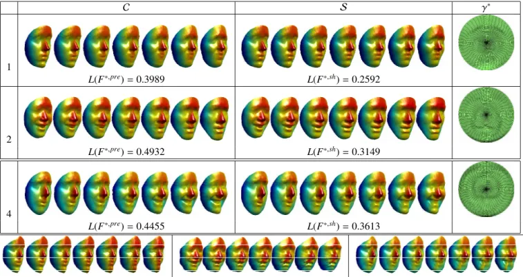
sion classes. Using these estimates one can form a generative
147
3D face model that can be used for random sampling.
148
(4) We provide tools for symmetry analysis of 3D faces, which
149
allows quantification of asymmetry of a given face and
identifi-150
cation of the nearest (approximately) symmetric face.
151
(5) We study expression and identity classification under this
152
framework using the defined metric. We compare our
perfor-153
mance to the state-of-the-art method in [13]. The main idea
154
behind presenting this application is to showcase the benefits of
155
an elastic framework in the recognition task. We leave a more
156
thorough study of classification performance and comparisons
157
to other state-of-the-art methods as future work.
158
The rest of this paper is organized as follows. Section 2
de-159
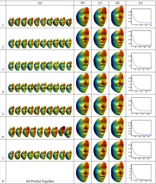
fines the mathematical framework. Section 3 presents the
appli-160
cability of the proposed method to various 3D face processing
161
tasks. We close the paper with a brief summary in Section 4.
162
2. Mathematical Framework
163
In this section, we describe the main ingredients in defining
164
a comprehensive, elastic shape analysis framework for facial
165
surfaces. We note that these methods have been previously
de-166
scribed for the case of quadrilateral, spherical and cylindrical
167
surfaces in [20, 21]. We extend these methods to
hemispheri-168
cal surfaces and apply them to statistical shape analysis of 3D
169
faces. Let F be the space of all smooth embeddings of a closed
170
unit disk in R3, where each such embedding defines a
parame-171
terized surface f : ¯D! R3
. Let Γ be the set of all
boundary-172
preserving diffeomorphisms of ¯D. For a facial surface f 2 F ,
173
f ◦ γrepresents its re-parameterization. In other words, γ is a
174
warping of the coordinate system on f . As previously shown
175
in [20], it is inappropriate to use the L2 metric for analyzing
176
shapes of parameterized surfaces, because Γ does not act on
177
F by isometries. Thus, we utilize the square-root normal field
178
(SRNF) representation of surfaces and the corresponding
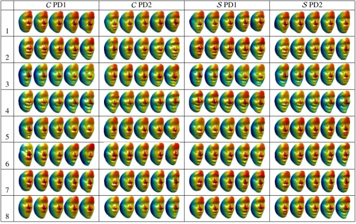
Rie-179
mannian metric proposed in [20]. We summarize these methods
180
next and refer the reader to those papers for more details.
181
Let s = (u, v) 2 ¯D define a polar coordinate system on the
182
closed unit disk. The SRNF representation of facial surfaces is
183
then defined using a mapping Q : F ! L2as Q( f )(s) = n(s)
|n(s)|1/2. 184
Here, n(s) = ∂ f∂u(s) ⇥∂ f∂v(s) denotes a normal vector to the
sur-185
face f at the point f (s). The space of all SRNFs is a subset
186
of L2( ¯D, R3), henceforth referred to simply as L2, and it is
187
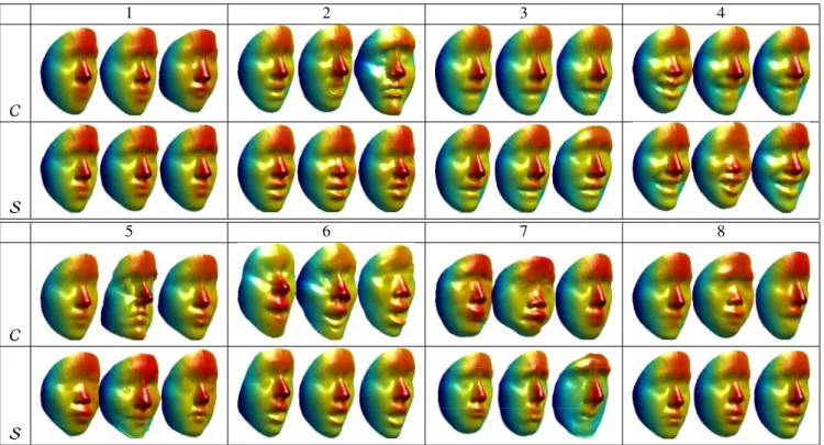
endowed with the natural L2 metric. The differential of Q is
188
a smooth mapping between tangent spaces, Q⇤, f : Tf(F ) !
189
TQ( f )(L2), and is used to define the corresponding Riemannian
190 metric on F as hhw1, w2iif = hQ⇤, f(w1), Q⇤, f(w2)iL2, where 191 w1, w2 2 Tf(F ), nw(s) = ∂ f ∂u(s) ⇥ ∂w ∂v(s) + ∂w ∂u(s) ⇥ ∂ f ∂v(s), | · | 192
denotes the 2-norm in R3, and ds is the Lebesgue measure
193
on ¯D [21]. Using this expression, one can verify that the
re-194
parameterization group Γ acts on F by isometries, i.e.
195
hhw1◦ γ, w2◦ γiif ◦γ = hhw1, w2iif. Another advantage of this
196
metric is that it has a natural interpretation in terms of the amount
197
of stretching and bending needed to deform one surface into
198
another. For this reason, it has been referred to as the partial
199
elastic metric [20]. Furthermore, this metric is automatically
200
invariant to translation. Scaling variability can be removed by
201
rescaling all surfaces to have unit area. We let C denote the
202
space of all unit area surfaces. This defines the pre-shape space
203
in our analysis.
204
Rotation and re-parameterization variability is removed from
205
the representation space using equivalence classes. Let q =
206
Q( f ) denote the SRNF of a facial surface f . A rotation of f
207
by O 2 S O(3), O f , results in a rotation of its SRNF
repre-208
sentation, Oq. A re-parameterization of f by γ 2 Γ, f ◦ γ,
209
results in the following transformation of its SRNF: (q, γ) =
210
(q ◦ γ)p Jγ, where Jγ is the determinant of the Jacobian of γ.
211
Now, one can define two types of equivalence classes, [ f ] =
212
{O( f ◦γ)|O 2 S O(3), γ 2 Γ} in C endowed with the metric hh·, ·ii
213
or [q] = {O(q, γ)|O 2 S O(3), γ 2 Γ} in L2endowed with the L2
214
metric; each equivalence class represents a shape uniquely in
215
its respective representation space. This results in two
strate-216
gies to account for the rotation and re-parameterization
vari-217
abilities in 3D face data. Given two surfaces f1, f2 2 C, the
218
exact solution comes from the following optimization
prob-219
lem: (O⇤, γ⇤) = arginf
(O,γ)2S O(3)⇥ΓdC( f1, O( f2◦ γ)).
Unfortu-220
nately, there is no closed form expression for the geodesic
dis-221
tance dC because of the complex structure of the Riemannian
222
metric hh·, ·ii. There is a numerical approach, termed
path-223
straightening, which can be used to compute this geodesic
dis-224
tance, but it is computationally expensive. Thus, we use an
225
approximate solution to the registration problem in our
analy-226
sis, which can be computed using the SRNF representation as
227
(O⇤, γ⇤) = arginf(O,γ)2S O(3)⇥Γkq1− (Oq2, γ)k. This problem is
228
much easier to solve and provides a very close approximation
229
to the original problem, because the partial elastic metric on C
230
is the pullback of the L2metric from the SRNF space.
231
The optimization problem over S O(3) ⇥ Γ is solved
itera-232
tively using the general procedure presented in [20, 21]. First,
233
one fixes γ and searches for an optimal rotation over S O(3)
234
using Procrustes analysis; this is performed in one step using
235
singular value decomposition. Then, given the computed
rota-236
tion, one searches for an optimal re-parameterization in Γ using
237
a gradient descent algorithm, which requires the specification
238
of an orthonormal basis for Tγid(Γ). The definition of this basis
239
depends on the domain of the surface. In the present case, we
240
seek a basis of smooth vector fields that map the closed unit
241
disk to itself. In order to define this basis, we make a small
242
simplification. Because all of the initial, facial surface
parame-243
terizations were obtained by defining the point s = (0, 0) at the
244
tip of the nose, we treat this point as a landmark, i.e. it is fixed
245
throughout the registration process. Given this simplification,
246
we first construct a basis for [0, 1] as B[0,1] ={sin(2πn1u), 1 −
247
cos(2πn1u), u, 1 − u|n1 =1, . . . , N1, u 2 [0, 1]} and a basis for
248
S1as B
S1={sin(n2v), 1 − cos(n2v), v, 2π − v|n2=1, . . . , N2, v 2 249
[0, 2π]}. We take all products of these two bases while
en-250
suring that the boundary of the unit disk is preserved. Then,
251
to define an orthonormal basis of Tγid(Γ) we use the
Gram-252
Schmidt procedure. This results in a finite, orthonormal basis
253
BD¯ = {b1, . . . , bN} for Tγid(Γ). In the following sections, we
254
let f2⇤ = O⇤( f2 ◦ γ⇤), where O⇤ 2 S O(3) is the optimal
rota-255
tion and γ⇤ 2 Γ is the optimal re-parameterization. Then, the
256
geodesic distance in the shape space S = C/(S O(3)⇥Γ) is
com-257
puted using d([ f1], [ f2]) = inf(O,γ)2S O(3)⇥ΓdC( f1, O( f2◦ γ)) ⇡
258
dC( f1, O⇤( f2◦ γ⇤)). This allows us to compute the geodesic only
259
once, after the two facial surfaces have been optimally
regis-260
tered.
261
As a next step, we are interested in comparing facial surface
262
shapes using geodesic paths and distances. As mentioned
ear-263
lier, there is no closed form expression for the geodesic in C,
264
and thus, we utilize a numerical technique termed
path-265
straightening. In short, this approach first initializes a path
be-266
tween the two given surfaces, and then “straightens” it
accord-267
ing to an appropriate path energy gradient until it becomes a
268
geodesic. We refer the reader to [22, 21] for more details. In
269
the following sections, we use F⇤,preto denote the geodesic path
270
between two facial surfaces f1and f2in the pre-shape space (no
271
optimization over S O(3) ⇥ Γ) and F⇤,sh to denote the geodesic
272
path in the shape space between f1 and f2⇤. The length of the
273
geodesic path is given by L(F⇤) = R1
0 p⌦hF ⇤ t, Ft⇤↵iFdt, where 274 F⇤ t = dF⇤
dt . All derivatives and integrals in our framework are
275
computed numerically. The computational cost of the proposed
276
method is similar to that reported in [22].
277
3. Applications
278
In this section, we describe the utility of the presented
math-279
ematical tools in various 3D face processing tasks including
280
deformation, template estimation, summarization of
variabil-281
ity, random sampling and symmetry analysis. We also present
282
two classification tasks concerned with (1) classifying
expres-283
sions, and (2) classifying person identities. The 3D faces used
284
in this paper are a subset of the BU-3DFE dataset. BU-3DFE
285
is a database of annotated 3D facial expressions, collected by
C S γ⇤ 1 L(F⇤,pre) = 0.3989 L(F⇤,sh) = 0.2592 2 L(F⇤,pre) = 0.4932 L(F⇤,sh) = 0.3149 4 L(F⇤,pre) = 0.4455 L(F⇤,sh) = 0.3613
Figure 1: Top: Comparison of geodesic paths and distances in C and S for different persons and expressions (1 neutral to anger, 2 happiness to disgust, and 3 sadness to happiness) as well as optimal re-parameterizations (allow elastic deformations between 3D faces). Bottom: Geodesics (1)-(3) computed using [13].
Yin et al. [23] at Binghamton University in Binghamton, NY,
287
USA, which was designed for research on 3D human faces and
288
expressions and to develop a general understanding of human
289
behavior. There are a total of 100 subjects in the database, 56
fe-290
males and 44 males. A neutral scan was first captured for each
291
subject. Then, each person was asked to perform six
expres-292
sions reflecting the following emotions: anger, happiness, fear,
293
disgust, sadness and surprise. The expressions varied
accord-294
ing to four levels of intensity (low, middle, high and highest).
295
Thus, there were 25 3D facial expression models per subject
296
in the entire database. We use a subset of this data with
high-297
est expression intensities (most challenging case) to assess the
298
proposed method.
299
Each facial surface is represented by an indexed collection
300
of radial curves that are defined and extracted as follows. The
301
reference curve on a facial surface f is chosen to be the
verti-302
cal curve after the face has been rotated to the upright position.
303
Then, each radial curve βαis obtained by slicing the facial
sur-304
face by a plane Pαthat has the nose tip as its origin and makes
305
an angle α with the plane containing the reference curve. We
306
repeat this step to extract radial curves at equally-separated
an-307
gles, resulting in a set of curves that are indexed by the angle α.
308
Thus, the facial surface is represented in a polar (radius-angle)
309
coordinate system. We use 50 radial curves sampled with 50
310
points in our surface representation (50 ⇥ 50 grid).
311
Face Deformation: We generate facial shape deformations
us-312
ing geodesic paths. While linear interpolations could also be
313
used here, the geodesic provides the optimal deformation under
314
the defined Riemannian metric. Since we only have to
com-315
pute the geodesic once per deformation, after the surfaces have
316
been optimally registered, this does not result in a prohibitive
317
computational cost. We compare the results obtained in C to
318
those in S in Figure 1. We consider three different examples
319
for various persons and expressions. There is a large decrease
320
in the geodesic distance in each case due to the additional
opti-321
mization over S O(3) ⇥ Γ. It is clear from this figure that elastic
322
matching of 3D faces is very important when the main goal is to
323
generate natural deformations between them. This is especially
324
evident in the areas of the lips and eyes. Take, for instance,
325
Example 1. In the pre-shape space, the lips are averaged out
326
along the geodesic path and are pretty much non-existent close
327
to the midpoint. But, due to a better matching of geometric
fea-328
tures along the geodesic path in the shape space, the lips are
329
clearly defined. The same can be observed in the eye region.
330
As will be seen in the next section, these distortions become
331
even more severe when one considers computing averages and
332
variability within a set of 3D faces. In the right panel of the
fig-333
ure we display the optimal re-parameterizations that achieve the
334
correspondence between these surfaces; these are clearly
non-335
linear and depict natural transformations. We also generated
336
geodesics for the same examples using the curve-based method
337
in [13] (bottom panel of Figure 1). These results suggest that
338
considering the radial curves independently can generate severe
339
distortions in the geodesic paths and produce unnatural
defor-340
mations between 3D faces.
341
Face Template: We generate 3D face templates using the
no-342
tion of the Karcher mean. Tools and results for computing
343
shape statistics for cylindrical surfaces under the SRNF
rep-344
(a) (b) (c) (d) (e) 1 10 20 30 40 0.23 0.24 0.25 0.26 2 10 20 30 40 0.26 0.28 0.3 0.32 3 10 20 30 40 0.3 0.32 0.34 4 10 20 30 0.26 0.28 0.3 0.32 0.34 5 10 20 30 0.2 0.21 0.22 6 10 20 30 40 0.24 0.25 0.26 0.27 0.28 7 10 20 30 40 0.23 0.24 0.25 0.26
8 All Pooled Together 10 20 30 40
2.6 2.7 2.8 2.9 3
Figure 2: (a) Sample of surfaces used to compute the face template for each expression: (1) anger, (2) disgust, (3) fear, (4) happiness, (5) neutral, (6) surprise, (7) sadness, and (8) all samples pooled together. (b) Sample average computed in C. (c) Karcher mean computed in S. (d) Karcher mean computed using [13]. (e) Optimization energy in S (sum of squared distances of each shape from the current average) at each iteration.
resentation have been previously described in [24]; we review
345
some of the concepts relevant to current analysis in the
fol-346
lowing sections. Let { f1, . . . , fn} 2 C denote a sample of
fa-347
cial surfaces. Then, the Karcher mean is defined as [ ¯f] =
348 argmin[ f ]2S Pn i=1L(F ⇤,sh i ) 2, where F⇤,sh
i is a geodesic path
be-349
tween a surface Fi⇤,sh(0) = f and a surface in the given sample
350
Fi⇤,sh(1) = fi⇤ that was optimally registered to f . A
gradient-351
based approach for finding the Karcher mean is given in [24].
352
The Karcher mean is actually an equivalence class of surfaces
353
and we select one element as a representative ¯f 2[ ¯f]. As one
354
can see from this formulation, the computation of the Karcher
355
mean requires n geodesic calculations per iteration. This can
356
be very computationally expensive, and thus, we approximate
357
the geodesic using a linear interpolation when computing the
358
facial surface templates. We present all results in Figure 2. We
C PD1 C PD2 S PD1 S PD2 1 2 3 4 5 6 7 8
Figure 3: The first two principal directions of variation (PD1 and PD2) computed in the pre-shape (C) and shape (S) spaces for expressions (1)-(8) in Figure 2.
compare the facial template computed in S to a standard sample
360
average computed in C and the curve-based Karcher mean [13].
361
First, we note from panel (e) that there is a large decrease in
en-362
ergy in each example. The qualitative results also suggest that
363
the 3D face templates computed in S are much better
represen-364
tatives of the given data than those computed in C or using the
365
curve-based method. Again, the biggest differences are
notice-366
able around the mouth and eyes. In fact, when looking at panels
367
(b) and (d), it is fairly difficult to recognize the expression; this
368
distinction is much clearer in panel (c).
369
Summary of Variability and Random Sampling: Once the
370
sample Karcher mean has been computed, the evaluation of the
371
Karcher covariance is performed as follows. First, we optimally
372
register all surfaces in the sample to the Karcher mean ¯f,
re-373
sulting in { f1⇤, . . . , fn⇤}, and find the shooting vectors {ν1, . . . , νn}
374
from the mean to each of the registered surfaces. The
covari-375
ance matrix K is computed using {νi}, and principal directions
376
of variation in the given data can be found using standard
prin-377
cipal component analysis (singular value decomposition). Note
378
that due to computational complexity, we do not use the
Rie-379
mannian metric hh·, ·ii to perform PCA; thus, we sacrifice some
380
mathematical rigor in order to improve computational efficiency.
381
The principal singular vectors of K can then be mapped to a
sur-382
face f using the exponential map, which we approximate using
383
a linear path; this approximation is reasonable in a
neighbor-384
hood of the Karcher mean. The results for all eight samples
385
displayed in Figure 2 are presented in Figure 3. For each
ex-386
ample, we display the two principal directions of variation in
387
C and S. These paths are sampled at −2, −1, 0, 1, 2 standard
388
deviations around the mean. The summary of variability in the
389
shape space more closely resembles deformations present in the
390
original data. This leads to more parsimonious shape models.
391
In contrast to the principal directions seen in C, the ones in S
392
contain faces with clear facial features.
393
Given a principal component basis for the tangent space
394
T[ ¯f](S), one can sample random facial shapes from an
approx-395
imate Gaussian model. A random tangent vector is generated
396 using v = Pk j=1zjpSj juj, where zj iid ⇠ N(0, 1), Sj j is the vari-397
ance of the jth principal component, and ujis the corresponding
398
principal singular vector of K. A sample from the approximate
399
Gaussian is then obtained using the exponential map frand =
400
expf¯(v), which again is approximated using a linear path. The
401
results are presented in Figure 4. As expected, the facial
sur-402
faces sampled in the shape space are visually preferred to those
403
sampled in the pre-shape space; this is due to better matching
404
of similar geometric features across 3D faces such as the lips,
405
eyes and cheeks.
406
Symmetry Analysis: To analyze the level of symmetry of a
fa-407
cial surface f we first obtain its reflection ˜f = H(v) f , where
408
H(v) = (I − 2vvvTTv) for a v 2 R
3
. Let F⇤,sh be the geodesic
409
path between f and ˜f⇤ = O⇤( ˜f ◦ γ⇤). We define the length of
410
the path F⇤,shas a measure of symmetry of f , ρ( f ) = L(F⇤,sh).
411
If ρ( f ) = 0 then f is perfectly symmetric. Furthermore, the
412
halfway point along the geodesic, i.e. F⇤,sh(0.5), is
approx-413
imately symmetric (up to numerical errors in the registration
414
and geodesic computation). If the geodesic path is unique, then
415
1 2 3 4 C S 5 6 7 8 C S
Figure 4: Random samples generated from the approximate Gaussian distribution in the pre-shape (C) and shape (S) spaces for expressions (1)-(8) in Figure 2.
(a) f and ˜f (b) Geodesic Path F⇤,sh (c) F⇤,sh(0.5)
1 ρ( f ) = 0.1626, ρ(F⇤,sh(0.5)) = 0.0177 2 ρ( f ) = 0.1041, ρ(F⇤,sh(0.5)) = 0.0100 3 ρ( f ) = 0.1405, ρ(F⇤,sh(0.5)) = 0.0159
Figure 5: (a) Facial surface f in blue and its reflection ˜f in red. (b) Geodesic path in S between f and ˜fand the measure of symmetry ρ( f ). We also compute the measure of symmetry for the midpoint of the geodesic ρ(F⇤,sh(0.5)), which is expected to be 0 for perfectly symmetric faces. (c) Midpoint of the geodesic.
amongst all symmetric shapes, F⇤,sh(0.5) is the closest to f in
416
S. Three different examples are presented in Figure 5. The
417
average measure of symmetry for the geodesic midpoints
(av-418
eraged over all of the presented examples) is 0.0145, which is
419
very close to 0 (perfect symmetry). In the presented
exam-420
ples, the faces are already fairly symmetric. Nonetheless, the
421
symmetrized faces (right panel) have a natural appearance with
422
clearly defined facial features.
423
Identity and Expression Classification: In the final
applica-424
tion, we explore the use of the proposed framework in two
425
different classification tasks. We compare our results to the
426
method presented in [13], which reported state-of-the-art
recog-427
nition performance in the presence of expressions. We do not
428
compare our performance to any other state-of-the-art methods
because many of them are specifically designed for
classifica-430
tion experiments (feature based). Our framework is more
gen-431
eral as it also allows deformation and statistical modeling of
432
faces. The proposed framework can be tuned to maximize
clas-433
sification performance by extracting relevant elastic features
434
from the computed statistical models, but we believe that this
435
is beyond the scope of the current paper.
436
Figure 6: Identity recognition in C (blue), S (red), and using [13] (green).
The first task we consider is concerned with classifying
ex-437
pressions. We selected 66 total surfaces divided into six
expres-438
sion groups (11 persons per group): anger, disgust, fear,
happi-439
ness, surprise and sadness. We computed the pairwise distance
440
matrices in C, S, and using [13]. We calculated the
classifi-441
cation performance in a leave-one-out manner by leaving out
442
all six expressions of the test person from the training set. The
443
classification accuracy in C was 62.12% while that in S was
444
74.24%. The classification accuracy of [13] was 68.18%. This
445
result highlights the benefits of elastic shape analysis of
hemi-446
spherical surfaces applied to this recognition task. It also
sug-447
gests that considering the radial curves independently, as done
448
in [13], deteriorates the recognition performance. The second
449
task we considered was identity classification irrespective of the
450
facial expression. Here, we added 11 neutral expression facial
451
surfaces (one per person) to the previously used 66 and
com-452
puted 11⇥66 distance matrices in C, S, and using the method in
453
[13]. We performed classification by first checking the identity
454
of the nearest neighbor. This resulted in a 100% classification
455
rate for all methods. Figure 6 shows the classification results
456
when accumulating over more and more nearest neighbors (up
457
to six since there are six total expressions for each person). It
458
is clear from this figure that identity classification in the shape
459
space is far superior to that in the pre-shape space. The
addi-460
tional search over Γ allows for the expressed faces to be much
461
better matched to the neutral faces, and in a way provides
“in-462
variance” to facial expressions in this classification task. The
463
performance of the proposed method is comparable to [13].
464
4. Summary and Future Work
465
We defined a Riemannian framework for statistical shape
466
analysis of hemispherical surfaces and applied it to various 3D
467
face modeling tasks including morphing, averaging, exploring
468
variability, defining generative models for random sampling,
469
and symmetry analysis. We considered two classification
ex-470
periments, one on expressions and one on person identities, to
471
showcase the benefits of elastic shape analysis in this
applica-472
tion. This leads us to several directions for future work. First,
473
we will investigate the use elastic facial shape features, which
474
can further improve the reported classification accuracy.
Sec-475
ond, we will utilize the proposed 3D face shape models as priors
476
in processing corrupted or incomplete raw data obtained from
477
3D scanners. Third, we want to study expression transfer via
478
parallel transport. These tools have not yet been developed for
479
hemispherical surfaces, and to the best of our knowledge, there
480
exist very few automatic methods for this task. Finally, we want
481
to move toward the difficult problem of modeling 3D dynamic
482
faces.
483
References
484
[1] Deng Z, Chiang P, Fox P, Neumann U. Animating blendshape faces by
485
cross-mapping motion capture data. In: Interactive 3D Graphics. 2006, p.
486
43–8.
487
[2] Huang H, Chai J, Tong X, Wu H. Leveraging motion capture and 3D
488
scanning for high-fidelity facial performance acquisition. ACM Trans
489
Graphics 2011;30(4):74:1–74:10.
490
[3] Lin I, Ouhyoung M. Mirror MoCap: Automatic and efficient capture of
491
dense 3D facial motion parameters from video. The Visual Computer
492
2005;21(6):355–72.
493
[4] Kakadiaris IA, Passalis G, Toderici G, Murtuza MN, Lu Y,
Karampatzi-494
akis N, et al. Three-dimensional face recognition in the presence of facial
495
expressions: An annotated deformable model approach. IEEE Trans
Pat-496
tern Analysis and Machine Intelligence 2007;29(4):640–9.
497
[5] Sandbach G, Zafeiriou S, Pantic M. Local normal binary patterns for
498
3D facial action unit detection. In: International Conference on Image
499
Processing. 2012, p. 1813–6.
500
[6] Lu X, Jain AK. Deformation modeling for robust 3D face matching. In:
501
Computer Vision and Pattern Recognition. 2006, p. 1377–83.
502
[7] Bouaziz S, Wang Y, Pauly M. Online modeling for realtime facial
ani-503
mation. ACM Trans Graphics 2013;32(4):40.
504
[8] Weise T, Bouaziz S, Li H, Pauly M. Realtime performance-based facial
505
animation. ACM Trans Graphics 2011;30(4):77.
506
[9] Gupta S, Aggarwal JK, Markey MK, Bovik AC. 3D face recognition
507
founded on the structural diversity of human faces. In: Computer Vision
508
and Pattern Recognition. 2007,.
509
[10] Wang Y, Liu J, Tang X. Robust 3D face recognition by local shape
dif-510
ference boosting. IEEE Trans Pattern Analysis and Machine Intelligence
511
2010;32(10):1858–70.
512
[11] Tsalakanidou F, Tzovaras D, Strintzis MG. Use of depth and colour
513
eigenfaces for face recognition. Pattern Recognition Letters
2003;24(9-514
10):1427–35.
515
[12] Bronstein AM, Bronstein MM, Kimmel R. Three-dimensional face
recog-516
nition. International Journal of Computer Vision 2005;64(1):5–30.
517
[13] Drira H, Ben Amor B, Srivastava A, Daoudi D, Slama R. 3D face
recog-518
nition under expressions, occlusions, and pose variations. IEEE Trans
519
Pattern Analysis and Machine Intelligence 2013;35(9):2270–83.
520
[14] Srivastava A, Klassen E, Joshi SH, Jermyn IH. Shape analysis of elastic
521
curves in Euclidean spaces. IEEE Trans Pattern Analysis and Machine
522
Intelligence 2011;33(7):1415–28.
523
[15] Ben Amor B, Drira H, Berretti S, Daoudi M, Srivastava A. 4-D facial
524
expression recognition by learning geometric deformations. IEEE Trans
525
Cybernetics 2014;44(12):2443–57.
526
[16] Samir C, Srivastava A, Daoudi M, Kurtek S. On analyzing symmetry
527
of objects using elastic deformations. In: International Conference on
528
Computer Vision Theory and Applications. 2009, p. 194–200.
529
[17] Sorkine O, Alexa M. As-rigid-as-possible surface modeling. In:
Sympo-530
sium on Geometry Processing. 2007, p. 109–16.
531
[18] Kilian M, Mitra NJ, Pottmann H. Geometric modeling in shape space.
532
ACM Trans Graphics 2007;26(3):64.
533
[19] Zhang Z, Li G, Lu H, Ouyang Y, Yin M, Xian C. Fast
as-isometric-as-534
possible shape interpolation. Computers & Graphics 2015;46(0):244 –56.
535
[20] Jermyn IH, Kurtek S, Klassen E, Srivastava A. Elastic shape matching
536
of parameterized surfaces using square root normal fields. In: European
537
Conference on Computer Vision. 2012, p. 804–17.
538
[21] Samir C, Kurtek S, Srivastava A, Canis M. Elastic shape analysis of
539
cylindrical surfaces for 3D/2D registration in endometrial tissue
charac-540
terization. IEEE Trans Medical Imaging 2014;33(5):1035–43.
541
[22] Kurtek S, Klassen E, Gore J, Ding Z, Srivastava A. Elastic geodesic paths
542
in shape space of parameterized surfaces. IEEE Trans Pattern Analysis
543
and Machine Intelligence 2012;34(9):1717–30.
544
[23] Yin L, Wei X, Sun Y, Wang J, Rosato MJ. A 3D facial expression database
545
for facial behavior research. In: Automatic Face and Gesture Recognition.
546
2006, p. 211–6.
547
[24] Kurtek S, Samir C, Ouchchane L. Statistical shape model for simulation
548
of realistic endometrial tissue. In: International Conference on Pattern
549
Recognition Applications and Methods. 2014,.
![Figure 6: Identity recognition in C (blue), S (red), and using [13] (green).](https://thumb-eu.123doks.com/thumbv2/123doknet/11633455.306229/9.892.190.300.260.355/figure-identity-recognition-c-blue-red-using-green.webp)
