A collaborative demand forecasting process with event-based fuzzy judgements

HAL Id: hal-00862940

https://hal.archives-ouvertes.fr/hal-00862940

Submitted on 17 Sep 2013

HAL is a multi-disciplinary open access

archive for the deposit and dissemination of sci-entific research documents, whether they are pub-lished or not. The documents may come from teaching and research institutions in France or abroad, or from public or private research centers.

L’archive ouverte pluridisciplinaire HAL, est destinée au dépôt et à la diffusion de documents scientifiques de niveau recherche, publiés ou non, émanant des établissements d’enseignement et de recherche français ou étrangers, des laboratoires publics ou privés.

A collaborative demand forecasting process with

event-based fuzzy judgements

Naoufel Cheikhrouhou, François Marmier, Omar Ayadi, Philippe Wieser

To cite this version:

Naoufel Cheikhrouhou, François Marmier, Omar Ayadi, Philippe Wieser. A collaborative demand forecasting process with event-based fuzzy judgements. Computers & Industrial Engineering, Elsevier, 2011, 61 (2), pp.409 - 421. �10.1016/j.cie.2011.07.002�. �hal-00862940�

A collaborative demand forecasting process with event-based

fuzzy judgments

Naoufel Cheikhrouhoua, François Marmierb, Omar Ayadia, Philippe Wieserc,

a Ecole Polytechnique Fédérale de Lausanne (EPFL), Laboratory for Production Management and Processes, Station 9, 1015 Lausanne, Switzerland

b Université de Toulouse, MINES ALBI – CGI, 81013 Albi, France

c Ecole Polytechnique Fédérale de Lausanne (EPFL), CDM, MTEI, Odyssea, Station 5, 1015 Lausanne, Switzerland

Abstract

Mathematical forecasting approaches can lead to reliable demand forecast in some environments by extrapolating regular patterns in time-series. However, unpredictable events that do not appear in historical data can reduce the usefulness of mathematical forecasts for demand planning purposes. Since forecasters have partial knowledge of the context and of future events, grouping and structuring the fragmented implicit knowledge, in order to be easily and fully integrated in final demand forecasts is the objective of this work. This paper presents a judgemental collaborative approach for demand forecasting in which the mathematical forecasts, considered as the basis, are adjusted by the structured and combined knowledge from different forecasters. The approach is based on the identification and classification of four types of particular events. Factors corresponding to these events are evaluated through a fuzzy inference system to ensure the coherence of the results. To validate the approach, two case studies were developed with forecasters from a plastic bag manufacturer and a distributor belonging to the food retailing industry. The results show that by structuring and combining the judgements of different forecasters to identify and assess future events, companies can experience a high improvement in demand forecast accuracy.

Keywords: Collaborative forecasting; Demand planning; Judgement; Time series; Fuzzy logic

1 Introduction

Time-series based forecasting is defined as the extrapolation of patterns from historical data to obtain an approximation of the future demand over a time horizon. Many forecasting methodologies have been developed based on different mathematical and statistical methods (Makridakis et al. 1998). Although mathematical approaches can lead to reliable demand forecasts in some contexts, extrapolating regular patterns only to predict specific and time-limited events can generate bad forecasts. Assuming that forecasters and salesmen have partial knowledge of the context, they can identify potential future events. This implicit knowledge cannot be used by statistical methods as it may correspond to specific events, such as a personnel strike, limited promotions or the opening of new facilities. It is recognized that a judgment based on contextual knowledge is a mandatory component of forecasting (Lawrence et al. 2006).

Additionally, there is still a need for work that will help companies improve their forecast quality using contextual and judgemental information from the different actors both at the enterprise as well as at the supply chain levels (Cheikhrouhou and Marmier 2010, Sanders and Ritzman 1995). Information can be fed into to the models using different approaches: The Bayesian approach requires explicit formulation of a model and conditioning on known quantities in order to draw inferences about unknown ones (Harvey 1991). Furthermore, the intervention analysis approach (also referred to as impact study) is based on the study of the effect of known events on time series. Intervention (or dummy) variables can be used in regression models to measure the effect of these events (Box et al. 1994, Chapter 13).

In the context of high uncertainty, it is beneficial to efficiently integrate judgmental and mathematical methods in order to take advantage, on the one hand, of the capacity of the company‟s actors to anticipate changes and integrate their domain knowledge, and on the other hand of the strength of mathematical forecasting models. For instance, in defining product priorities in a forecasting process, Meunier Martins et al. (2005) take into account contextual information on lead times, component commonalities and product criticalities. Franses (2008) considers the integration of contextual information in the downstream part of the forecasting process, where different combinations of judgemental and mathematical forecasts are possible. Furthermore, it has been proved that, in most cases, collaborative forecasting gives better results than a process with a single input (Aviv 2007). Indeed, collaborative forecasting refers to different situations, where people and systems interact and cooperate to form a process aiming at producing good forecasts. The literature on collaborative forecasting falls into two categories. The first category addresses issues related to inter-firm forecasting among partners participating in a supply structure such as supply chain, collaborative network, extended enterprise, etc. (Barratt and Oliveira 2001, McCarthy and Golicic 2002, Poler et al. 2008, Raghunathan 1999). The second category explores the intra-firm collaborative forecasting process that takes into consideration the achievement of forecasts with the help of different units or departments within the same firm (Ireland and Bruce 2001, Windischer et al. 2009). Only few works address group-oriented intra-firm processes, mainly due to the difficulties in ensuring the coherence between different decision makers.

In the intra-firm collaborative forecasting process addressed in this work, different forecasters use their judgements in order to modify initial mathematical forecasts and deliver a final common adjusted plan. The aim of this work is to develop a collaborative forecasting approach to improve the accuracy by structuring and efficiently exploiting the knowledge of the different forecasters in fuzzy information. The process presented consists of is a judgmental adjustment approach, combining a mathematical model with event-based judgmental factors. In this approach, the mathematical model provides initial forecasts. Based on identified judgemental factors, the forecasters structure their knowledge, related to internal and external information on the industrial and commercial contexts, and adjust the mathematical forecasts using a fuzzy rule-based system. The approach is then compared in its accuracy to pure mathematical methods, naïve forecasts and event-based adjusted processes with a single forecaster, using common error measures. Furthermore, the approach is validated by two industrial case studies, a plastic bag manufacturer in Spain and a fresh food distributor in France.

In section 2, an overview of the literature on demand forecasting techniques, integrating both mathematical and judgemental processes is provided. Section 3 outlines the details of the proposed collaborative judgmental adjustment-based approach and its main features through the development of the fuzzy system. The error measures used to assess the quality of the approach are proposed in section 4. Details of the two industrial case studies using the developed approach are provided in section 5 along with a comparative study of the performances. Finally, section 6 details the conclusions of this work and the future research directions.

2 Forecasting methods integrating judgemental and mathematical processes

There exist four main types of demand forecasting approaches integrating human judgment into structured processes: (a) model building, (b) forecast combination, (c) judgemental decomposition and (d) judgemental adjustment (Webby and O‟Connor 1996). The model building approach uses judgment in the selection and development of the quantitative forecast (Bunn and Wright 1991). Forecasting methods based on the combination of judgemental information and mathematical models require high technical knowledge and constitute a pragmatic approach for integrating the personal analysis of contextual information that may influence the forecasts (Fildes and Goodwin 2007). Sanders and Ritzmann (1995) show that although this method gives good results for time-series with a low variation coefficient, both (mathematical and contextual) forecasts have similar accuracies.

The judgemental decomposition consists of identifying and analysing the effects of past contextual information in time-series before developing mathematical models. Once the mathematical forecasts are achieved, factors related to possible future events are taken into account and the forecasts are then adjusted based on human judgement (Edmundson 1990). Judgemental decomposition is more complex than combination or adjustment methods, but it may bring a good structure when integrating judgement. From the demand planner point of view, judgemental decomposition could reduce the cognitive workload but may also be risky and ineffective in some circumstances. Indeed, the multiplicative reconstruction of decomposed components increases the risk of errors and thus, good results are not guaranteed.

In the judgemental adjustment process, the mathematical forecasts are reviewed by experts and then adjusted on the basis of their knowledge and experiences. Judgemental adjustment is a common practice in companies and constitutes the major alternative to the combination process. However, this practice is criticised because of its informal nature (Bunn and Wright 1991). In fact, using a procedure or a decision support system to structure the information is helpful for decision making, where the effectiveness of unstructured processes such as graphical adjustment may be dependent on the quality of the reference forecasts (Willemain 1991, 1989). Furthermore, it is proven that structured forecasting processes lead to improvements in accuracy (Harvey 2007, Vanston 2003, Lawrence et al. 1985). In particular, for judgmental adjustments, it is shown that the structured approach is efficient (Marmier and Cheikhrouhou 2010). Sanders and Ritzmann (2004) report the advantages of this approach such as time saving, allowing the judgment to rapidly incorporate the latest updated information. Flores et al. (1992) compare different approaches of judgemental adjustment. The forecaster ranks the impacts due to different factors to obtain an average adjustment of an ARIMA forecast. Similarly, Lee et al. (1990) define different event-based factors to determine the future demand in different situations. However, these factors have only been formally used in artificial neural networks in order to identify different specific events and eliminate their influences from time-series (Lee and Yum 1998, Nikolopoulos and Assimakopoulos 2003). The high potential they offer in structuring the judgement and providing efficient collaborative forecasting systems has been neglected (Nikolopoulos et al. 2007). The issue of structuring the implicit information and judgement is addressed by Marmier and Cheikhrouhou (2010), who propose an event-based method for judgemental adjustment. The developed approach uses knowledge, from a single forecaster, structured around the classification of probable future events into four classes of factors. From the different works on capturing and incorporating the knowledge, Collopy and Armstrong (1992) develop a rule-based procedure to determine how the model and its parameters should be chosen. However, not only the system is complex but it also does not address the issues related to diversion of perception between forecasters in collaborative forecasting. In this topic, Fildes et al. (2009) report in a case study on forecasts achieved using a judgemental adjustment approach and the influence of positive or negative perceptions on the accuracy. They show that positive adjustments in demand planning are much less likely to improve the accuracy than negative

adjustments. Indeed, forecasters‟ optimism could add bias to the information that leads to bad forecasts. This phenomenon can be reduced if collaborative techniques are used. In fact, Wright and Rowe (2011) report that group-based judgemental forecasting methodologies could lead to a global consensus. Kerr and Tindale (2011) argue that only aggregation methods facilitating information exchange between group members are likely to be beneficial over a statistical averaging of prior individual opinions. Such information exchange in structured group interactions provides the enabling conditions for group members to identify errors in the justifications of judgments. Additionally, Önkal et al. (2011) show that group discussions and decision making may be efficient methods of displaying and solving differential contingencies, leading to group forecasts that outperform initial forecasts. Moreover, they highlight that a group-based judgemental adjustment tends to improve the accuracy of both the statistical average of the forecasts and the pure model-based forecast. On this side, providing additional information and different approaches, such as fuzzy modelling, improves the accuracy (Kabak and Ulengin 2010, Petrovic et al. 2006). In addition, in situations where forecasters might be biased, it is important to obtain forecasts from experts with different biases (Armstrong et al. 2008).

In this paper, we propose a new collaborative approach integrating human judgments to mathematical models in a structured way. The work is based on future event identification and classification to assist forecasters in focusing selectively on specific events and in structuring their judgments when adjusting forecasts. Therefore, each forecaster can easily communicate his implicit knowledge concerning future evolution of the markets (total volume, number of competitors…), customers (their numbers, needs, potential demand…) or contractors (development status, special offers…) by representative factors. Since the occurrence of these factors as events is uncertain, a fuzzy logic model is adopted to formalise and characterise the factors and their weights. A weight is defined as the impact of the corresponding event on the future demand. The collaborative process relies upon fuzzy rules using inputs from the different in-firm forecasters and providing global adjustments.

3 Collaborative demand forecasting with event-based fuzzy judgments

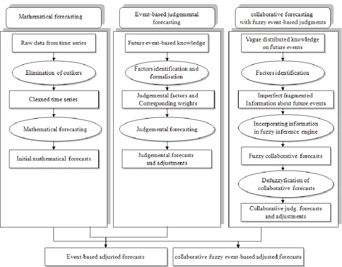
Since the different forecasters involved in a process may have different perceptions of similar events, we propose to take into consideration these differences to improve the forecast accuracy. The collaborative process consists of integrating the judgements of several forecasters and structuring the information using complementarities of the different perceptions. Practically, the forecasters take part in a (real or virtual) meeting and use their experiences and knowledge in a structured manner to build up the forecasts. The proposed process is composed of four phases: First, mathematical forecasts are produced based on cleaned data (data where outliers are identified and eliminated). Second, factors are identified and classified using the forecasters‟ knowledge related to future events. Third, the different information collected is integrated into a fuzzy inference engine to obtain a global fuzzy judgement. The global fuzzy adjustments are then defuzzified. Finally, the mathematical forecasts are adjusted using defuzzified adjustments. Figure 1 shows this approach where the collaborative fuzzy event-based adjusted forecasts are obtained by the combination of initial mathematical forecasts (left side of the figure) and collaborative forecasts with fuzzy event-based judgments (right side of the figure). The results of the proposed approach are compared to the classical mathematical approaches as well as to the event-based adjusted approach (combination of mathematical forecasts and event-based judgmental forecasts), which takes advantage of the knowledge of a single forecaster (Marmier and Cheikhrouhou 2010).

[insert figure 1 about here]

- The forecasters have (different or similar) perceptions of future events that may impact the demand over one or several time periods.

- Every forecaster is considered as reasonable and responsible (rationality assumption) and therefore their propositions are well-intentioned.

- The uncertainty considered is only related to the event occurrence and its amplitude.

3.1 Development of initial mathematical forecasts

The initial forecasts are developed on the basis of a standard statistical and mathematical process. Indeed, a filtering process relying upon a decomposition technique (Makridakis et al. 1998) consists of: 1- identifying real outliers, 2- replacing outliers by representative values, and 3- fitting the time series with a mathematical model.

Grubbs (1969) defines an outlier as an observation that deviates significantly from all other observations of a data sample. In fact, outliers could exist in time series as an unusual or erroneous data observation or entry. An outlier should be analysed in detail by the forecasters in order to decide to replace it in the time-series, if it is a classical outlier, or to keep it if the related event occurred can be explained. Testing the existence of an outlier and removing it consists of verifying whether the corresponding value in the time series belongs to a tolerance interval. Every observation of the time-series outside this interval is rejected and replaced by another representative value, such as the average of the neighbouring values. The Grubbs‟ test (Grubbs 1950) based on the Student tables compares outlying data points with the average and standard deviation of a set of data and then allows to detect outliers. The past observations of the time-series are filtered over the horizon K (noted , k= K, K-1,…,0), and the corresponding mathematical forecasts are defined in Equation 1.

(1)

where is the forecast based on cleaned data for the period t.

To derive mathematical forecasts, traditional statistical/mathematical models such as random walk (Collopy and Armstrong 1972), exponential smoothing (Gardner 2006), ARIMA (Box and Jenkins 1976) or structural time series (Harvey and Shephard 1993) can be used. The best model to select for a considered situation depends on the nature of the products and the business, the nature of data, the aggregation level, the forecast horizon, the shelf life of the model and the expected accuracy. Therefore, common patterns are taken into account for the development of the mathematical model. Indeed, the trend, the seasonality, the periodicity, the serial correlation, the skewness, and the kurtosis have been widely used as criteria in many time series feature-based research (Armstrong 2001). Selecting the best model is highly non-trivial and has received considerable attention with different approaches being studied (Zou and Yang 2004). We briefly discuss the approaches that are closely related to our work, assuming that the work of De Gooijer et al. (1985) can be considered for a review on this topic. Moreover, different „checklists‟ have been developed for the selection of the best forecasting method in a given situation (Chambers et al. 1971, Reid 1972, Georgoff and Murdick 1986). This idea has been enhanced by several authors to design expert systems, such as the Rule-based Forecasting that automatically selects and proposes the adapted forecasting method (Wang et al. 2009). Furthermore, even if the corresponding literature is rich, basic rules leading to the choice of the most adequate approach can be mentioned; The Single Exponential Smoothing model is adequate for data series without trend and where the forecasts are developed on a short-term horizon. Holt's model is used for short term forecasting based on time series that present trends without any seasonal factors. On the other side, the Holt-Winter's model can be used to provide forecasts presenting trend and seasonality. In the case of time series presenting trend, the ARIMA model could be used. The

latter is a general class of models that includes random walk, random trend, and exponential smoothing models as special cases. Where simple models could work well, combination of candidate models can reduce the instability of the forecast and improve the accuracy (Yang 2004).

Moreover, each observation presents particularities that modify the adequacy between the series and the model, requiring checking and validating the chosen model by an accuracy measurement. The accuracy is measured by dividing the data set into two sets. The first one is used to test several models by best fitting the data and the second set is kept to assess the quality of the fit. In order to measure the error, the forecast residuals, expressed by the Sum of Squared Errors (SSE), measuring the importance of huge errors is used. Additionally, different error measures can be used, e.g. the Mean Error (ME), the Mean Squared Error (MSE), the Mean of the Percentage (MPE), the Mean Absolute Error (MAE), the Absolute Percentage Errors (MAPE) and the Theil's U-statistics.

3.2 From a distributed knowledge to collaborative judgmental forecasts

Lee and Yum (1998) define a judgmental factor as a “factor that cannot be fully incorporated into the time series models, and thus cannot be effectively identified by the extrapolation of past patterns in the data set”. Depending on the studied case, a factor attribute or causal variable can be: duration, intensity, type, etc. The occurrence of the judgmental factor is considered as a judgmental event, characterized by its impact that may affect the demand over one time period or more. Different categories of factors are defined with respect to the cause of the event, such as the market, which consists of external factors influencing the demand and its characteristics, the clients, through their specific needs, the contractors, who may occasionally propose special offers and promotions, the specific weather conditions, etc.

In this work, four types of judgmental factors are considered: transient factors, quantum jump factors, transferred impact factors and trend change factors. They allow to take into account most of the common situations of demand pattern change. Each factor, consequence of a causal variable, is the basis for a corresponding adjustment. Since an adjustment has an impact on the initial forecast over time, each adjustment, resulting from one or several judgmental factors, is noted F(i,t) (the adjustment value), where i is the total impact and t is time. The impact i can reach its maximum value . The variable does not prejudge whether the event will occur or not. It only expresses the probable maximal value. Assuming that N forecasters are participating in a forecasting meeting, they firstly reach a consensus in assigning a value to the maximum impact . Secondly, each forecaster expresses his opinion by giving a weight wj (j=1…N) on a scale from 0 to 100%, representing the effect of the occurrence of the considered event in the future with respect to . This evaluation can vary from a forecaster to another. If a forecaster estimates that the effect will not impact the forecasts, the individual weighting can be described as 0% of , contrary to a high impact that can be assessed as close to 100%. It is also the case when a forecaster is uncertain about the occurrence of a possible event, where a neutral opinion is then possible. In that case, only the information provided by the remaining forecasters is taken into account as input to the fuzzy inference system.

3.3 Fuzzy collaborative adjustment system

Since each forecaster has a different perception on future probable events, depending on his partial knowledge, activity sector, geographical location, etc., providing precise and complete information on the future demand is a difficult task. Evaluations are then made using fuzzy linguistic variables. Indeed, an input is represented by a membership function associated to the

fuzzy set {very low, low, medium, high, very high}. The membership function (MF) describes the degree of adherence of the corresponding input value for each element of the fuzzy set. Figure 2 shows the MFs taken as input basis for the assessment, where triangular MFs are chosen for the designed fuzzy system. Indeed, triangular MFs are appropriate for representing human judgments since they attribute different membership values for two given degrees of criterion satisfaction.

[insert figure 2 about here]

A Fuzzy Inference System (FIS) is then designed and developed. This system uses IF-THEN rules formulated on the basis of:

- the statements provided by the forecasters in the considered enterprises studied in this work, and - a consensus achievement, where the final weight of each identified probable future event results from the group decision-making process.

The “OR” and “AND” connectors are considered when formulating the IF-THEN rules since different inputs have to be taken into account in a same rule. The FIS using the Mamdani method (Mamdani and Assilian 1999) aggregates the outputs of the fuzzy rules and generates a defuzzified value w for the global weight using the centroid method. This final weight is then considered in the adjustment process for the factor under study using Equation 2.

(2)

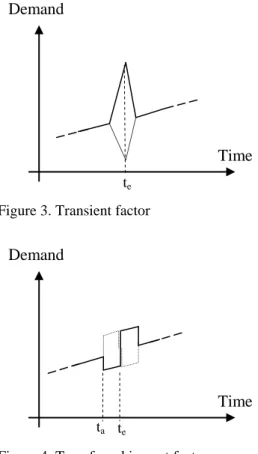
3.4 Classification schema of the judgemental factors and event occurrences 3.4.1 Transient factors

The transient factors influence time series only during the period in which a particular event occurs (cf. time te in figure 3).

[insert figure 3 about here]

Assuming that time can be decomposed into periods tp, the total impact i covers the effective number of impacted periods (t1,...,tn). Adjustments encompassing n consecutive time periods are calculated using Equation 3:

(3)

where f represents the periodical adjustments and ip corresponds to the intensity at the impacted period tp. Transient factors can change the value of the main initial trend

^

0

Y , either in a decreasing or an increasing way. After establishing the sign of the adjustment (positive or negative), the forecasters reach a consensus to determine . According to his knowledge, each forecaster j deduces a weight wj which is provided to the FIS to calculate the final weight.

3.4.2 Transferred impact factors

In case of a transferred impact factor, the global impact i is transferred from a set of periods Sp1 to another one Sp2, without changing the global forecast over the horizon. Figure 4 shows an example of this factor. This phenomenon is observed for instance when price changes are announced beforehand at time ta (for example, when suppliers want to reduce their inventories and thus introduce special offers). In this case, the temporary change in demand due to the expected price change is transferred and compensated in the following time period at time te.

[insert figure 4 about here]

Adjustments encompassing n consecutive periods are calculated by equation 4.

(4)

where ip is the (positive or negative) impact of the factor during the time period p. The forecasters determine together to be transferred and, using the scale of impact, each forecaster proposes a weight wj for the probable considered event.

3.4.3 Quantum jump factors

As presented in figure 5, the quantum jump factor occurs when the effect of a non-repetitive event is permanent.

[insert figure 5 about here]

The adjustment calculation is detailed in equation 5.

(5)

Where Qj is a binary variable which means that the Y-intercept, which defines the elevation of the demand trend, is impacted by the intensity i at the effective date te, (date of the jth event that generates the demand jump).

If t < te then Qj =0 Otherwise Qj =1.

The weighting process here is similar to the other factors. After determining the adjustment sign, the forecasters have to determine and then, each forecaster expresses his opinion about the percentage that weights .

3.4.4 Trend change factors

Figure 6 shows a trend change factor that could for instance represent a price change. Most of the time, a price change is known a priori, and it is possible to forecast the trend change. If the forecaster provides contextual information, a regression of on can estimate the impact of price changes, where P(t) is the price at time t. Otherwise, forecasters establish the sign of the possible trend change and its limit . Then, each forecaster gives his own perception by weighting the impact. The trend adjustment is detailed in equation 6.

[insert figure 6 about here]

(6)

where Tc is a binary variable expressing if the slope of a linear regression of the demand trend is impacted with the intensity i at the effective date te, (the date of the event generating the demand jump):

otherwise, Tc =1.

3.5 Adjustment process

The obtained adjustment allows changing the initial mathematical forecasts and deriving the final collaborative adjusted forecasts, as represented in equation 7.

^ a

Y

where ^_Y( )t is the adjustment calculated with the collaborative approach. It corresponds to the

total impact of the different events occurring at time t on demand. When multiple judgmental factors simultaneously impact the demand, it is necessary to take into account forecast adjustments according to the effects of each individual judgmental event. Then, the global adjustment at time t, defined in equation 8, corresponds to the sum of the different adjustments related to the K factors impacting the demand at time t.

(8)

4 Evaluation of adjusted forecast quality

Armstrong (2001) stated that, in the case of integrating human knowledge in forecasting processes, some error measures are not particularly useful to forecasters with business expertise and their use is probably more harmful when using time-series. Based on these statements, two forecast error measures are selected in this work: the Mean Absolute Error (MAE) and the Mean Absolute Percentage Error (MAPE). Indeed, the use of MAE enables highlighting both positive and negative errors. With MAE, the total magnitude of error is provided but not the real bias or the error direction. MAPE measures the deviation as a percentage of the actual data with respect to the forecasts. Thus, positive and negative errors do not cancel out. Consider Yt as the actual value at period t, for t = 1…T, and Ft as the forecast for this period, the MAE is given by equation (9) and the MAPE is given by equation (10).

1 t t M A E e T 







Moreover, we compare our work to additional benchmark models by providing the two naïve models. The first one, called Naïve Forecast 1 (NF1) consists of taking the last actual value and using it as forecast for all the next periods. The second model, Naïve Forecast 2 (NF2) takes the last actual value as forecast for all the next periods, but integrates the seasonal pattern of the time series. The Theil's U-statistics have a number of interesting properties that could be used to assess the quality of a forecasting technique. They do not provide information on the forecasting bias which is captured by the mean error. Both of its instances, labelled U1 in Equation 11 and U2 in Equation 12, are used in this work. The U1 statistic is bounded between 0 and 1. The more accurate the forecasts, the lower the value of the U1 statistic. Considering U2, values less than 1 indicate high forecasting accuracy for the considered model compared to the naïve forecasting (Makridakis et al. 1998, chapter 2).

(11)

(12)

5 Industrial case studies

Two real industrial case studies are used to assess the practical usefulness of the proposed forecasting approach: a plastic bag manufacturer and a distributor from the food industry. In both cases, three forecasters proceed to structure and integrate their implicit knowledge into mathematical models.

5.1 Presentation of the first case study: Forecasting plastic bag demand

The proposed approach is applied to the case of the Company X, a plastic bag manufacturer based in the south of Spain. The polyethylene bag market is analyzed and the demand is forecasted. The time series used are composed of the aggregated monthly demand collected over three years (2004-2006), as it can be observed in figure 7. The aim of this study is to plan the demand for the year 2007. Company X has three main customers in this area, all of which are supermarkets. Three forecasters from the company X analyze the historical data and the factors influencing plastic bag demand and then forecast the specific events based on their respective knowledge.

[insert figure 7 about here]

The first step consists of cleaning the data by outlier elimination. In our case, the Grubb‟s test shows an outlier observed at t = 29 months. This observation, outside the tolerance interval, is considered as an outlier and is replaced by the average of its two neighbouring values. The cleaned time series is presented in figure 7.

5.2 Initial mathematical forecasts

The literature offers good references for the selection of the best mathematical model that fits the best the time series. The reader is referred to Makridakis et al. (1998) for a complete description of those models. In the case of the plastic bags manufacturer, the time series presents a strong trend as shown in figure 7. Moreover, due to the increase in demand for plastic bags during the months preceding summer and Christmas holidays, a weak seasonality is observed in the historical data. Based on these observations, a short list of pertinent mathematical models is developed by the industrial forecasters participating to the study, containing ARIMA (Autoregressive Integrated Moving Average) and Holt-Winters. Indeed, the forecasters intentionally limit the list to two candidates: Holt-Winters as adequate models for data presenting

seasonality and ARIMA as the most used and representative technique in time series forecasting, according to them. To select the most adapted one, their respective fitness to the time series is calculated using the Web-reg software, an ARIMA Add-in for Excel (Web-reg 2010), and the “stats” package of R (R-project 2010) for the Holt-Winters model. An important aspect in developing mathematical models, in particular those based on Autoregressive and Moving Average techniques, is related to the identification of their orders. Indeed, fitting the model consists of identifying the parameters of the best model representing the data. In order to identify if the time series is a good candidate for an ARIMA model, different methods are used (Ong et al. 2005, Hannan and Rissanen 1982, Akaike 1974, Akaike 1981, Kadane and Lazar 2004). Among these methods, the Box–Jenkins method is a univariate time series consisting of different steps: identification, estimation and testing, and application to forecasting (Box and Jenkins 1976, Makridakis et al. 1998, chapter 7). The Box-Jenkins method can handle either stationary or non-stationary time series, both with and without seasonal elements (Lim and McAleer 2002). However, even if Box–Jenkins method is widely used, its practical implementation proves to be complex. As a consequence, simple procedures can be adopted, such as minimizing the Akaike Information Criterion (AIC) (Akaike 1974, Akaike 1981), the Schwarz criterion (Schwarz 1978) or other related criteria (Hannan and Quinn 1979). To solve the minimization problem for the identification of the best model fitting the data, different techniques are available. One of the most efficient techniques is the Levenberg–Marquardt algorithm (Bertsekas 1995). Indeed, the latter is a standard technique used to determine the values of the parameters that minimize the sum of the squared residual values for a set of observations. The Levenberg-Marquardt algorithm is the core engine of the Web-reg software (2010) for the identification of ARIMA model parameters. This software is selected and used by the forecasters in the first case study to identify the parameters of the ARIMA model that best fits the available data.

The obtained forecasts (over a period of 12 months) for the Holt-Winters model present a higher Sum of Squared Errors (SSE equal to 409165) than the ARIMA(5,0,4) model (SSE equal to 201852). The forecast error for the Holt-Winters model, as a seasonal model is higher too (MAE is equal to 134 and MAPE is equal to 0.102), than for the ARIMA(5,0,4) model (MAE equal to 112.2 and MAPE equal to 0.0819). Figure 8 presents the forecasts obtained with the ARIMA(5, 0, 4) method for 2007, which is retained by the industrial experts as the initial mathematical model.

[insert figure 8 about here]

5.3 Subjective adjustments

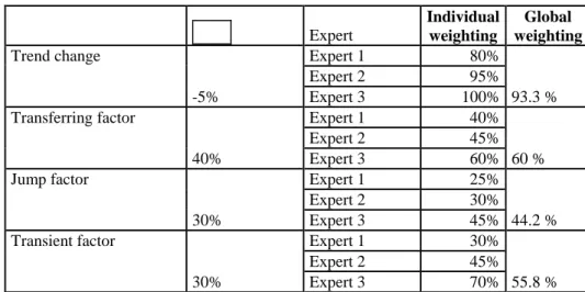
The three forecasters of the company X identify future events and classify the different corresponding factors as transient, transferring, jump or change trend factors. Then, during a meeting, a consensus is reached by these forecasters on the maximum impact for each factor. Based on this value, a weight is attributed to each causal variable by each forecaster. By using this process, the different opinions are integrated and the adjustment is made. In this case study, the forecasters propose that the following factors would influence the future demand.

Plastic price: The forecasters predict that the demand trend will change since the raw materials

price will increase starting in January 2007 due to new framework contracts with the suppliers. The plastic price is then the causal variable related to the trend change factor.

The trend is computed using the method of the least squares with a regression line. Each forecaster weights the corresponding trend line change. Then the assessments are introduced to the fuzzy inference system which provides the collaborative judgemental forecast and adjustments.

Assume that P(t) is the price at time t and Y(t) is the demand at time t. A regression of

on estimates the impact of price changes as shown in equation 13.

(13) To adjust the trend, the initial trend is firstly removed from the forecast, the price impact is secondly identified, the new trend is then calculated and finally, the new trend is added to the forecast.

[insert table 1 about here]

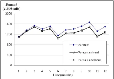
As presented in table 1, the maximum impact is a trend decrease of 5%. Each forecaster participating in the meeting gives his opinion concerning the impact as a percentage of this value. Three inputs are considered 80 %, 95 % and 100 % and introduced into the FIS which gives a trend adjustment of -4.6 % (93.3 % of –5 %). The forecast without trend and the adjusted forecast are given in figure 9.

[insert figure 9 about here]

Special offer: The forecasters predict that their company will have too much inventory in the

beginning of 2007. For this reason, a special offer is planned, proposing lower prices to their clients if they order higher quantities than usual. The consequence of this factor is that a major part of the demand of February and March 2007 will be transferred to January. The special offer is classified as a transferring factor. Indeed, this factor depends on the proposed price in the special offers and on the holding costs.

The special offer is made to the three main customers. The forecasters determine that the demand increase (related to the special offer) will represent at the maximum level 40 % of the monthly consumption. Each forecaster expresses his perception by weighting it individually by 40 %, 45 % and 60 % as shown in Table 1. The global weight given by the FIS is 60 %. The results of the rating in table 1 show that the forecasters predict a demand increase for January.

Plastic bag improvements: Technical changes in plastic bags by Company X are under

consideration in order to fulfil the ISO 14000 requirements (environmental regulations). The forecasters predict that using ecological non-polluting plastic bags is an interesting Marketing criterion to present to the supermarkets. The demand would then increase, classifying the factor as a jump factor, since the concept would attract new clients. Here, the causal variable is the demand volume of the new clients interested in ecological plastic bags.

Company X detected a potential client (Client 5) for the biodegradable plastic bags. The company decided then to make an experimental change in their raw materials based on a new generation of biodegradable substances, during the two summer months. The forecasters expect that this change will not impact the current basis of clients, but rather attract Client 5. Then, the forecasters state that the client‟s interest would increase the global demand to a maximum level of 30 % (cf. Table 1). After having expressed their weights (respectively 30 %, 45 % and 70 %), the FIS gives a final adjustment of 44.2 % of .

Client situations: Client 3, a client of the company X, posting regular orders with fixed

quantities of plastic bags per month, announced that its facilities would close for a month after the summer holidays for maintenance purposes. A logical consequence of this event would be a decrease in the demand. However, according to the forecasters, this client will order more items

to fill his stocks. This case shows the importance of the relationship between the client and the supplier and the role of human factors in demand planning. The factor is classified as a transient factor. As presented in Table 1, reaches 30 %. Based on the forecasters‟ opinions, the FIS gives an adjustment of 55.8 % of .

Table 2 presents the total impact of the different forecasted factors on the demand per month using the information from table 1. It is then possible to compare the adjustments proposed by a single forecaster (the right side values obtained from (Marmier and Cheikhrouhou 2010)) and those obtained using three different opinions for each event considered (the left side values).

[insert table 2 about here]

5.4 Collaborative adjusted forecasts

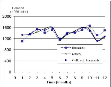
Figure 10 compares the real sales data in 2007 to the mathematical forecast as well as to the collaborative judgmental adjusted forecast.

[insert figure 10 about here]

Table 3 gives for each month the forecast error in product units and in percentage. It is clear that the adjusted forecasts present better results compared to the initial mathematical model since they are closer to the real sales for 10 out of 12 months.

[insert table 3 about here]

Table 4 presents the forecast performances of the proposed collaborative approach, measured using MAE, MAPE and both Theil's U-statistics U1 and U2. The collaborative adjusted forecast gives the best results since the MAE is decreased by 70% and the MAPE by 71%. In addition, the MAPE is about 0.02, which means that, in average, only a global error of 2% is made on the whole year. Moreover, this performance is illustrated by the U1 statistic that shows the lowest reported values, closer to 0. The U2 statistic, less than 1, shows that the collaborative adjustment approach outperforms the other approaches, notably the naïve forecast NF2, even if the latter integrates the same seasonal pattern of the time series.

[insert table 4 about here]

The historical data used to approximate the future demand do not contain the impact of non-periodic events, such as those that could be related to the four factor types. Therefore, it cannot logically lead to optimal forecasts. The adjustments help in minimizing the forecast errors. However, if the adjustments were done globally, without structuring or without a real analysis of their impacts, their durations and their durations over time, the deviation and the error could increase. Our approach is sufficiently simple to be used in practice. It is also complete enough to allow representative adjustments with respect to the industrial reality.

5.5 Second case study: Fresh Food Distribution

In this second application, we are interested in a set of 4 different products provided by a fresh food distributor with historical sales on different horizons (from 20 to 36 months) depicted on figures 11 to 14. The aim is to develop demand forecasts on a 6 month horizon for all considered products. For the different time series, the forecasters identified that the mathematical models are insufficient to achieve accurate forecasts. Different factors due to customers‟ demand behaviour

are considered without detailing the causal variables (several exceptionally high orders have been already announced by their customers). First, mathematical forecasts are generated on a horizon of 6 months, through the identification of the best models fitting the historical data (double exponential smoothing for the series shown in figures 11, 12 and 14 and Holt-Winters for the series of figure 13). The forecasts are then adjusted by a team of three forecasters from the company using the proposed approach. Table 5 presents the factors and the corresponding weights. For each time series, the different factors are presented in the second column of the table. The third column shows the value of of each event jointly determined by the forecasters. The crisp adjustment value obtained after defuzzification is presented in the last column of table 5. “Neutral” corresponds to the fact that a forecaster cannot give a weight to when he estimates having insufficient information relative to the event. In this case only two inputs are considered.

[insert table 5 about here]

The differences between mathematical forecasts and real sales show the limit of the past data extrapolation to obtain accurate forecasts (cf. Fig. 11 to 14); By using the structured forecaster judgements for the different identified factors and taking the advantage of several forecaster perceptions for the events considered, substantial improvements of the forecast accuracy were achieved.

[insert figure 11 about here]

[insert figure 12 about here]

[insert figure 13 about here]

[insert figure 14 about here]

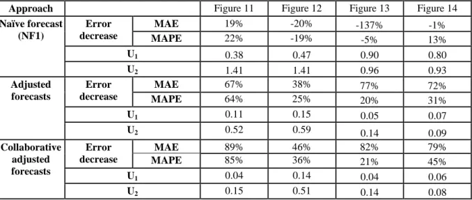
Table 6 shows the improvement of the error measures MAE and MAPE, expressed in percentage with respect to the performances of the mathematical models. In this second case study, the Naïve Forecast used (NF1), does not integrate any seasonal pattern since the time series does not present any seasonality. The resulting collaborative adjusted forecasts present better results considering both the MAE and MAPE. Indeed, an increase in forecast quality of at least 21% for each product is obtained, that reaches 80 %, compared to the mathematical model. Moreover, using the expertise of several forecasters leads to better results than using the knowledge of only one forecaster. Logically, this is explained by the fact that a single forecaster cannot always have the best opinion for each decision. Furthermore, this expert does not have a complete view of the market situation. The prism of vision is then larger by combining the perceptions of a group of experts. This good performance is confirmed by the U1 statistic results that are the lowest for the collaborative adjusted forecast and by the U2 values that are much less than 1. As a conclusion, this case study further proves the efficiency of the global approach to deliver forecasts with high accuracy as shown in the first case study. It is clear that the historical data used to approximate the future demand do not encompass the impact of non periodic events. Therefore, the collaborative adjusted approach logically leads to improved results.

6 Discussion and conclusions

The collaborative factor-based fuzzy approach presented in this paper helps groups of forecasters in structuring their judgments and providing global forecasts using an adjustment technique. Therefore, the forecasters are able to structure and communicate efficiently their relative and partial knowledge concerning the evolution of markets, customers and contractors using representative factors. The global approach consists mainly of three steps: a) data filtering and development of mathematical forecasting, b) factors formalisation and identification and c) collaborative adjustment process. This approach is applied to plan the demand of a manufacturing company and a fresh food distributor.

It is shown that the proposed forecasting method allows forecasters to identify different factors in order to integrate specific events and assess their impacts on demand. For both case studies presented, the proposed approach has a substantial impact on the accuracy of the resulting forecasts. In fact, the Mean Absolute Error and the Mean Absolute Percentage Error are both decreased in comparison with other techniques, thanks to the efficiency of the collaborative decision making system. Those results are confirmed by the Theil's U-statistics, thus translating the accuracy of the forecast obtained through the collaboration of forecasters. Compared to previous work, where additional information is extracted from time series and integrated to different decision support systems, our approach is original, as it bases the forecasting process on collaborative and structured judgements from knowledgeable forecasters. However, awareness in using such approaches has to be addressed. As the developed work is based on initial mathematical forecasts, the model that best fits the data is not always the one that provides the best forecasts. Accordingly, attention has to be paid to the selection of the initial forecasting model, in order to reduce the risk of providing knowledge to inappropriate statistical models. In developing case studies, the new process was appreciated by the forecasters since they can provide vague information without being committed with any single information they can provide. From a social point of view, the impact of introducing such a method cannot be neglected; the new approach decreases the pressure on forecasters in terms of providing accurate information, while it allows the company to capture the intrinsic knowledge of its experts for better forecast plans.

In the future, the development of a measure/indicator that reflects the different levels of uncertainty of the obtained collaborative forecast is under interest. In addition, studying the different individual forecaster perceptions and their contributions to the collaborative forecasting process, relying on their psychological profiles, is an interesting future research direction.

7 Acknowledgements

The authors would like to thank the Swiss innovation promotion agency (CTI) that funded the research project and the industrial partners for their collaboration. They also would like to address special thanks to M. Michael Ingram and Mrs Aoife Hegarty for their contribution to the improvement of the paper quality.

References

Akaike, H., 1974. A new look at the statistical model identification. IEEE Transactions on Automatic Control. 19 (6), 716–723.

Akaike, H., 1981. Likelihood of a model and information criteria. Journal of Econometrics, 16(1), 3-14.

Armstrong, J.S., Green, K.C., Soon, W., 2008. Polar Bear Population Forecasts: A Public-policy Forecasting Audit. Interfaces, 38, 382-405.

Armstrong, J. S. 2001. Judgmental bootstrapping: inferring expert rules for forecasting. In: J. S. Armstrong (Ed.), Principles of forecasting: A handbook for researchers and practitioners (pp. 171-192). Norwood, MA: Kluwer.

Aviv, Y., 2007. On the benefits of collaborative forecasting partnerships between retailers and manufacturers. Management Science. 53(5), 777-794.

Barratt, M., Oliveira, A. 2001. Exploring the experiences of collaborative planning initiatives. International Journal of Physical Distribution & Logistics Management. 31(4), 266–289.

Bertsekas, D.P., 1995. Nonlinear Programming. Athena Scientific: Belmont, MA.

Box, G. E. P., Jenkins, G. M., Reinsel, G. C., 1994. Time Series Analysis, Forecasting and Control, 3rd ed. Prentice Hall, Englewood Clifs, NJ.

Box, G.E.P, Jenkins, G.M., 1976. Time Series Analysis: Forecasting and Control, (2nd ed.), Holden-Day, San Francisco.

Bunn, D., Wright, G., 1991. Interaction of judgmental and statistical forecasting methods, issues and analysis. Management Science. 37(5), 501-18.

Chambers, J. C., Mullick, S. K., Smith, D. D., 1971. How to Choose the Right Forecasting Technique. Harvard Business Review 49, 45-71.

Cheikhrouhou, N., Marmier, F., 2010. Human and organisational factors in planning and control: Editorial. Production Planning and Control. 21(4), 345-346.

Collopy, F., Armstrong, J.S., 1992. Rule-Based Forecasting: Development and Validation of an Expert Systems Approach to Combining Time Series Extrapolations. Management Science. 38 (10), 1394-1414.

De Gooijer, J. G., Abraham, B., Gould, A., Robinson, L., 1985. Methods for determining the order of an autoregressive-moving average process: A survey. International Statistical Review A, 53, 301–329.

Edmundson, R. H., 1990. Decomposition; a strategy for judgemental forecasting. Journal of Forecasting. 9(4), 305-314.

Fildes, R., Goodwin, P., Lawrence, M., Nikolopoulos, K., 2009. Effective forecasting and judgmental adjustments: An empirical evaluation and strategies for improvement in supply-chain planning. International Journal of Forecasting. 25(1), 3-23.

Fildes, R., Goodwin, P., 2007. Good and bad judgement in forecasting: Lessons from four companies. Foresight. 8, 5-10.

Flores, B.E., Olson, D.L., Wolfe, C., 1992. Judgmental adjustment of forecasts: A comparison of methods. International Journal of Forecasting. 7(4), 421-433.

Franses, H.P., 2008. Merging models and experts. International Journal of Forecasting. 24(1), 31-33.

Gardner, Jr., E. S., 2006. Exponential smoothing: The state of the art-part II. International Journal of Forecasting. 22(4), 637-666.

Georgoff, D. M., Murdick, R. G., 1986. Manager‟s Guide to Forecasting. Harvard Business Review. 64, 110-120.

Grubbs, F.E., 1969. Procedures for detecting outlying observations in samples. Technometrics. 11, 1–21.

Grubbs, F.E., 1950. Sample criteria for testing outlying observations. The Annals of Mathematical Statistics. 21(1), 27–58.Hannan, E.J., Rissanen, J., 1982. Recursive estimation of mixed autogressive-moving average rder. Biometrika. 69 (1), 81–94.

Hannan, E. J., & Quinn, B. G., 1979. The determination of the order of an autoregression. Journal of the Royal Statistical Society, Series B. 41, 190– 195.

Harvey, A.C., 1991. Forecasting, Structural Time Series Models and the Kalman Filter, Cambridge Books, Cambridge University Press, ISBN 9780521405737.

Harvey, N., 2007. Use of heuristics: Insights from forecasting research. Thinking and Reasoning. 13(1), 5-24.

Harvey, A.C., Shephard, N., 1993. Structural time series models. In Maddala, G. S., Rao, C. R., and Vinod, H. D. (eds.), Handbook of Statistics, Volume 11. Amsterdam: Elsevier Science Publishers B V.

Ireland, R., Bruce, R., 2000. CPFR : only the beginning of collaboration. Supply chain management review. September-October, 80-88.

Kabak, O., Ülengin, F., 2010. A demand forecasting methodology for fuzzy environments. Journal of Universal Computer Science. 16(1), 121-139.

Kadane, J. B., Lazar, N. A., 2004. Methods and criteria for model selection. Journal of the American Statistical Association, 99(465), 279-290.

Kerr, N.L., Tindale, R.S., 2011. Group-based forecasting?: A social psychological analysis. International Journal of Forecasting. 27(1), 14-40.

Lawrence, M., Goodwin, P., O‟Connor, P., Önkal, D., 2006. Judgmental forecasting: A review of progress over the last 25 years. International Journal of Forecasting, 22, 493-518.

Lawrence, M., Edmundson, R.H., O‟Connor, M.J., 1985. An examination of the accuracy of judgmental extrapolation of time series. International Journal of Forecasting. 1(1), 25-35.

Lim, C., McAleer, M., 2002. Time series forecasts of international travel demand for Australia. Tourism Management, 23(4), 389-396.

Lee, J.K., Yum, C.S., 1998. Judgmental adjustment in time series forecasting using neural networks. Decision Support Systems. 22, 135-154.

Lee, J.K., Oh, S.B., Shin, J.C., 1990. UNIK-FCST: Knowledge-Assisted Adjustment of Statistical Forecasts. Expert Systems With Applications. 1, 39-49.

Makridakis, S., Wheelwright, S., Hyndman, R.J., 1998. Forecasting, methods and applications. John Wiley & Sons, Inc. (3rd ed.).

Mamdani, E. H., Assilian, S., 1999. Experiment in linguistic synthesis with a fuzzy logic controller. International Journal of Man-Machine Studies. 51, 135-147.

Marmier, F., Cheikhrouhou, N., 2010. Structuring and integrating human knowledge in demand forecasting: a judgmental adjustment approach, Production Planning and Control. 21(4), 399-412. Mc Carthy, T., Golicic, S., 2002. Implementing collaborative forecasting to improve supply chain performance. International journal of Physical Distribution and Logistics Management. 32(6), 431-454.

Meunier Martins, S., Cheikhrouhou, N., Glardon, R., 2005. Strategic analysis of products related to the integration of human judgment into demand forecasting. Integrating Human Aspects in Production Management. ZÜLCH, Gert; JAGDEV, Harinder S.; STOCK, Patricia (Eds.): New York: Springer, 157-171.

Nikolopoulos, K., Goodwin, P., Patelis, A., Assimakopoulos, V., 2007. Forecasting with cue information: A comparison of multiple regression with alternative forecasting approaches. European Journal of Operational Research. 180(1), 354-368.

Nikolopoulos, K., Assimakopoulos, V., 2003. Theta intelligent forecasting information system, Industrial Management and Data Systems. 103(8-9), 711-726.

Ong, C.-S., Huang J.-J., Tzeng, G.-H., 2005. Model identification of ARIMA family using genetic algorithms. Applied Mathematics and Computation. 164 (3), 885-912.

Önkal, D., Lawrence, M., Zeynep Sayim, K., 2011. Influence of differentiated roles on group forecasting accuracy. International Journal of Forecasting. 27(1), 50-68.

Petrovic, D., Xie, Y., Burnham, K., 2006. Fuzzy Decision Support System for Demand Forecasting with a Learning Mechanism. Fuzzy Sets and Systems. 157, 1713– 1725.

Poler, R., Hemandez J.E., Mula, J., Lario, F.C., 2008. Collaborative forecasting in networked manufacturing enterprises. Journal of Manufacturing Technology Management. 19(4), 514-528. R-project, 2010. Free software environment for statistical computing and graphics. http://www.r-project.org/, last access on September, 20th 2010.

Raghunathan, S., 1999. Interorganizational collaborative forecasting and replenishment systems and supply chain implications. Decision Sciences. 30(4), 1053-1071.

Reid, D. J., 1972. A Comparison of Forecasting Techniques on Economic Time Series. In: Forecasting in Action. OR Society.

Sanders, N.R., Ritzman, L.P., 2004. Integrating judgmental and quantitative forecasts: Methodologies for pooling marketing and operations information. International Journal of Operations & Production Management. 24 (5), 514-529.

Sanders, N.R., Ritzman, L.P., 1995. Bringing judgment into combination forecasts. Journal of Operations Management. 13(4), 311-321.

Schwarz, G. E., 1978. Estimating the dimension of a model. Annals of Statistics. 6 (2), 461–464. Tavanidou, E., Nikolopoulos, K., Metaxiotis, K., Assimakopoulos, V., 2003. eTIFIS: An innovative e-forecasting web application. International Journal of Software Engineering and Knowledge Engineering. 13(2), 215-236.

Vanston, J.H., 2003. Better forecasts, better plans, better results. Research Technology Management. 46(1), 47-58.

Wang, X., Smith-Miles, K., Hyndman, R., 2009, Rule induction for forecasting method selection: Meta-learning the characteristics of univariate time series. Neurocomputing. 72(10-12), 2581-2594.

Web-reg, 2010. ARIMA Add-in for Excel. http://www.web-reg.de/arma_addin.html, last access on September, 20th 2010.

Webby, R., O'Connor, M., Edmunson, B., 2005. Forecasting support systems for the incorporation of event information: An empirical investigation. International Journal of Forecasting. 21(3), 411-423.

Webby, R., O'Connor, M., 1996. Judgemental and statistical time series forecasting: a review of the literature. International Journal of Forecasting. 12(1), 91-118.

Willemain, T. R., 1991. The effect of graphical adjustment on forecast accuracy. International Journal of Forecasting. 7(2), 151-154.

Willemain, T.R., 1989. Graphical adjustment of statistical forecasts. International Journal of Forecasting. 5(2), 179-185.

Windischer, A., Grote, G., Mathier, F., Meunier Martins, S., Glardon, R., 2009. Characteristics and organizational constraints of collaborative planning. Cognition, Technology and Work. 11(2), 87-101.

Wright, G., Rowe, G., 2011. Group-based judgmental forecasting. An integration of extant knowledge and the development of priorities for a new research agenda. International Journal of Forecasting. 27 (1), 1-13.

Yang, Y., 2004. Combining forecasting procedures: Some theoretical results. Econometric Theory. 20(1), 176-222

Zou, H., Yang, Y., 2004. Combining time series models for forecasting. International Journal of Forecasting. 20(1), 69-84.

FIGURES

Figure 1. Conceptual scheme of the general method developed, the initial forecasts and the event-based adjusted approach

Figure 3. Transient factor

Figure 4. Transferred impact factor

Figure 5. Quantum jump factor

Figure 6. Trend change factor

Demand Time Demand ta te Demand Time te Time te Demand Time te

Figure 7. Historical demand of Company X (2004-2006)

Figure 8. Company X demand (2004-2007)

Figure 10. Mathematical forecasts, collaborative adjusted forecasts and reality 0 2000 4000 6000 8000 10000 12000 14000 16000 18000 20000 1 3 5 7 9 11 13 15 17 19 21 23 25 27 29 31 33 35 37 Data s erie Math. Forec. Real data Adjus t. forec. Coll. Adj. forec.

Figure 11. Jump factor identification

0 5000 10000 15000 20000 25000 30000 1 2 3 4 5 6 7 8 9 10 11 12 13 14 15 16 17 18 19 20 21 22 23 24 25 26 Data s erie Math. Forec. Real data Adjus t. forec. Coll. Adj. forec.

Figure 12. Transient factor identification on several time periods

0 5000 10000 15000 20000 25000 30000 35000 40000 1 2 3 4 5 6 7 8 9 10 11 12 13 14 15 16 17 18 19 20 21 22 23 24 25 26 27 28 29 Data s erie Math. Forec. Real data Adjus t. forec. Coll. Adj. forec.

Figure 13. Transient factor identification

0 10000 20000 30000 40000 50000 60000 70000 1 3 5 7 9 11 13 15 17 19 21 23 25 27 29 31 33 35 37 39 41 Data s erie Math. Forec. Real data Adjus t. forec. Coll. Adj. forec.

TABLES

Table 1. The different event impacts, their features and their weights

Month Trend change adjustment

Transferring factor adjustment Jump factor adjustment Transient factor adjustment TOTAL ADJUSTMENT January -19 / -23 264 / 400 244 / 377 February -37 / -46 -132 / -200 179 / 200 10 / -46 March -56 / -69 -132 / -200 179 / 200 -8 / -69 April -75 / -92 179 / 200 104 / 108 May -93 / -115 179 / 200 86 / 85 June -112 / -138 179 / 200 67 / 62 July -131 / -161 179 / 200 48 / 39 August -149 / -184 179 / 200 30 / 16 September -168 / -207 254 / -250 86 / -457 October -187 / -230 -187 / -230 November -205 / -253 -205 / -253 December -224 / -276 -224 / -276 Table 2. Final monthly adjustments (Collaborative judg. adjustments / judg. adjustments)

Forecast error Percentage error

Month Math. forecast Coll. Adj. forecast Reality Math. forecast Adjusted forecast Math. forecast Adjusted forecast 1 1106 1350 1322 216 28 0.16 0.021 2 1359 1369 1349 -10 20 -0.01 0.014 3 1539 1531 1436 -103 95 -0.07 0.066 4 1411 1515 1555 144 40 0.09 0.026 5 1513 1599 1608 95 9 0.06 0.006 6 1152 1219 1208 56 11 0.05 0.009 7 1372 1420 1341 -31 79 -0.02 0.059 8 1411 1441 1473 62 32 0.04 0.022 9 1512 1598 1604 92 6 0.06 0.004 10 1669 1482 1528 -141 46 -0.09 0.030 11 1325 1120 1131 -194 11 -0.17 0.010 12 1498 1274 1296 -202 22 -0.16 0.017 Table 3. Comparison of the forecasts and the errors for the year 2007

Expert Individual weighting Global weighting Trend change -5% Expert 1 80% 93.3 % Expert 2 95% Expert 3 100% Transferring factor 40% Expert 1 40% 60 % Expert 2 45% Expert 3 60% Jump factor 30% Expert 1 25% 44.2 % Expert 2 30% Expert 3 45% Transient factor 30% Expert 1 30% 55.8 % Expert 2 45% Expert 3 70%

Error measure _{MAE MAPE U1 U2} Mathematical forecast 112.20 0.0819 0.05 0.65

Naïve forecast (NF2) 64.81 0.0465 0.03 0.47

Adjusted forecast 97.54 0.0666 0.06 0.89

Collaborative adjusted forecast 33.91 0.0236 0.02 0.25 Table 4. Comparison of the error measures

Table 5. Experts opinions on event impacts

Approach Figure 11 Figure 12 Figure 13 Figure 14

Naïve forecast (NF1) Error decrease MAE 19% -20% -137% -1% MAPE 22% -19% -5% 13% U1 0.38 0.47 0.90 0.80 U2 1.41 1.41 0.96 0.93 Adjusted forecasts Error decrease MAE 67% 38% 77% 72% MAPE 64% 25% 20% 31% U1 0.11 0.15 0.05 0.07 U2 0.52 0.59 _{0.14 0.09} Collaborative adjusted forecasts Error decrease MAE 89% 46% 82% 79% MAPE 85% 36% 21% 45% U1 0.04 0.14 0.04 0.06 U2 0.15 0.51 0.14 0.08

Table 6. Improvement of the forecast accuracy for the case study Example Factors (parts) Expert

Individual weighting

Global weighting

Figure 11 Transient factor

-10000 Expert 1 25% 30 % Expert 2 30% Expert 3 Neutral Jump factor 60000 Expert 1 Neutral 92.5 % Expert 2 70% Expert 3 90% Figure 12 Transient factor

30000 Expert 1 45% 80.2 % Expert 2 60% Expert 3 90% Transient factor 30000 Expert 1 30% 40 % Expert 2 35% Expert 3 40% Figure 13 Transient factor

60000

Expert 1 5%

19.8 % Expert 2 10%

Expert 3 20% Figure 14 Transient factor

10000 Expert 1 40% 60 % Expert 2 85% Expert 3 Neutral Jump factor 10000 Expert 1 Neutral 60 % Expert 2 50% Expert 3 85%