Representation learning for dialogue systems

(1)

Université de Montréal

REPRESENTATION LEARNING FOR

DIALOGUE SYSTEMS

Par

Iulian Vlad Serban

Institut Québécois d’Intelligence Artificielle (Mila)

Département d’Informatique et de Recherche Opérationnelle (DIRO),

Faculté des Arts et des Sciences

Thèse présentée à la Faculté des arts et des sciences en vue de l’obtention du grade de

Philosophiœ Doctor (Ph.D.) en informatique.

mai 2019

R

(2)

(3)

Université de Montréal

Faculté des études supérieures et postdoctorales

Ce mémoire intitulé

REPRESENTATION LEARNING FOR

DIALOGUE SYSTEMS

Présenté par

Iulian Vlad Serban

a été évalué par un jury composé des personnes suivantes :

Alain Tapp (président-rapporteur) Aaron Courville (directeur de recherche) Yoshua Bengio (co-directeur de recherche) Pascal Vincent (membre du jury) Phil Blunsom

Department of Computer Science Oxford University

(4)

(5)

I

Sommaire

Cette thèse présente une série de mesures prises pour étudier l’apprentissage de représentations (par exemple, l’apprentissage profond) afin de mettre en place des systèmes de dialogue et des agents de conversation virtuels. La thèse est divisée en deux parties générales.

La première partie de la thèse examine l’apprentissage des représentations pour les modèles de dialogue génératifs. Conditionnés sur une séquence de tours à partir d’un dialogue textuel, ces modèles ont la tâche de générer la prochaine réponse appropriée dans le dialogue. Cette partie de la thèse porte sur les modèles séquence-à-séquence, qui est une classe de réseaux de neurones pro-fonds génératifs. Premièrement, nous proposons un modèle d’encodeur-décodeur récurrent hiérar-chique (“Hierarchical Recurrent Encoder-Decoder”), qui est une extension du modèle séquence-à-séquence traditionnel incorporant la structure des tours de dialogue. Deuxièmement, nous pro-posons un modèle de réseau de neurones récurrents multi-résolution (“Multiresolution Recurrent Neural Network”), qui est un modèle empilé séquence-à-séquence avec une représentation stochas-tique intermédiaire (une “représentation grossière”) capturant le contenu sémanstochas-tique abstrait com-muniqué entre les locuteurs. Troisièmement, nous proposons le modèle d’encodeur-décodeur récurrent avec variables latentes (“Latent Variable Recurrent Encoder-Decoder”), qui suivent une distribution normale. Les variables latentes sont destinées à la modélisation de l’ambiguïté et l’incertitude qui apparaissent naturellement dans la communication humaine. Les trois mod-èles sont évalués et comparés sur deux tâches de génération de réponse de dialogue: une tâche de génération de réponses sur la plateforme Twitter et une tâche de génération de réponses de l’assistance technique (“Ubuntu technical response generation task”).

La deuxième partie de la thèse étudie l’apprentissage de représentations pour un système de dialogue utilisant l’apprentissage par renforcement dans un contexte réel. Cette partie porte plus particulièrement sur le système “Milabot” construit par l’Institut québécois d’intelligence artifi-cielle (Mila) pour le concours “Amazon Alexa Prize 2017”. Le Milabot est un système capable de bavarder avec des humains sur des sujets populaires à la fois par la parole et par le texte. Le système consiste d’un ensemble de modèles de récupération et de génération en langage naturel, comprenant des modèles basés sur des références, des modèles de sac de mots et des variantes des modèles décrits ci-dessus. Cette partie de la thèse se concentre sur la tâche de sélection de réponse. À partir d’une séquence de tours de dialogues et d’un ensemble des réponses possi-bles, le système doit sélectionner une réponse appropriée à fournir à l’utilisateur. Une approche d’apprentissage par renforcement basée sur un modèle appelée “Bottleneck Simulator” est pro-posée pour sélectionner le candidat approprié pour la réponse. Le “Bottleneck Simulator” apprend un modèle approximatif de l’environnement en se basant sur les trajectoires de dialogue observées et le “crowdsourcing”, tout en utilisant un état abstrait représentant la sémantique du discours.

(6)

Le modèle d’environnement est ensuite utilisé pour apprendre une stratégie d’apprentissage du renforcement par le biais de simulations. La stratégie apprise a été évaluée et comparée à des ap-proches concurrentes via des tests A / B avec des utilisateurs réel, où elle démontre d’excellente performance.

Mots clés: apprentissage profond, apprentissage par renforcement, systèmes de dialogue, agents de conversation virtuels, les modèles de dialogue génératifs

(7)

II

Summary

This thesis presents a series of steps taken towards investigating representation learning (e.g. deep learning) for building dialogue systems and conversational agents. The thesis is split into two general parts.

The first part of the thesis investigates representation learning for generative dialogue models. Conditioned on a sequence of turns from a text-based dialogue, these models are tasked with gen-erating the next, appropriate response in the dialogue. This part of the thesis focuses on sequence-to-sequence models, a class of generative deep neural networks. First, we propose the Hierarchical Recurrent Encoder-Decoder model, which is an extension of the vanilla sequence-to sequence model incorporating the turn-taking structure of dialogues. Second, we propose the Multiresolu-tion Recurrent Neural Network model, which is a stacked sequence-to-sequence model with an intermediate, stochastic representation (a "coarse representation") capturing the abstract semantic content communicated between the dialogue speakers. Third, we propose the Latent Variable Re-current Encoder-Decoder model, which is a variant of the Hierarchical ReRe-current Encoder-Decoder model with latent, stochastic normally-distributed variables. The latent, stochastic variables are intended for modelling the ambiguity and uncertainty occurring naturally in human language com-munication. The three models are evaluated and compared on two dialogue response generation tasks: a Twitter response generation task and the Ubuntu technical response generation task.

The second part of the thesis investigates representation learning for a real-world reinforce-ment learning dialogue system. Specifically, this part focuses on the Milabot system built by the Quebec Artificial Intelligence Institute (Mila) for the Amazon Alexa Prize 2017 competition. Mi-labot is a system capable of conversing with humans on popular small talk topics through both speech and text. The system consists of an ensemble of natural language retrieval and genera-tion models, including template-based models, bag-of-words models, and variants of the models discussed in the first part of the thesis. This part of the thesis focuses on the response selection task. Given a sequence of turns from a dialogue and a set of candidate responses, the system must select an appropriate response to give the user. A model-based reinforcement learning approach, called the Bottleneck Simulator, is proposed for selecting the appropriate candidate response. The Bottleneck Simulator learns an approximate model of the environment based on observed dialogue trajectories and human crowdsourcing, while utilizing an abstract (bottleneck) state representing high-level discourse semantics. The learned environment model is then employed to learn a rein-forcement learning policy through rollout simulations. The learned policy has been evaluated and compared to competing approaches through A/B testing with real-world users, where it was found to yield excellent performance.

(8)

Keywords: deep learning, reinforcement learning, dialogue systems, conversational agents, gener-ative dialogue models

(9)

III

List of Tables

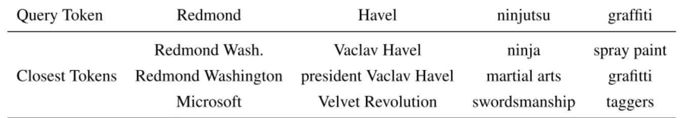
1 Examples of the closest tokens given by Skip-Gram model trained on 30 billion training words. This table was adapted from Mikolov et al. (2013b, p. 8). . . 17

2 Examples of query sentences and their nearest sentences of the Skip-Thought Vec-tors model trained on the Book Corpus dataset (Zhu et al., 2015). This table was extracted from Kiros et al. (2015, p. 3).. . . 20

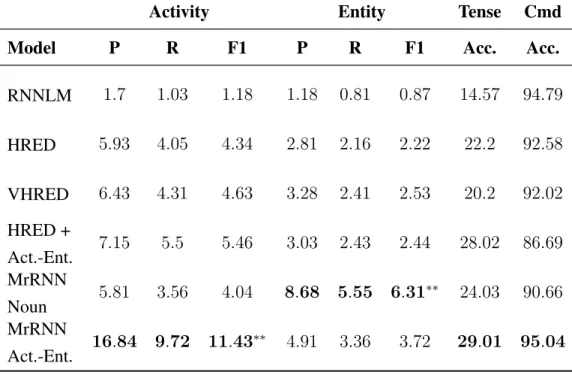
3 Ubuntu evaluation using precision (P), recall (R), F1 and accuracy metrics w.r.t. activity, entity, tense and command (Cmd) on ground truth utterances. The su-perscript ∗ indicates scores significantly different from baseline models at 95% confidence level. . . 57

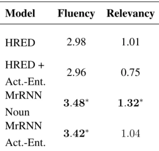
4 Ubuntu evaluation using human fluency and relevancy scores given on a Likert-type scale 0-4. The superscript∗ indicates scores significantly different from base-line models at 90% confidence level. The RNNLM and VHRED models are ex-cluded, since they were not part of the human evaluation. . . 58

5 Ubuntu model examples. The arrows indicate a change of turn. The examples were chosen from a set of short, but diverse dialogues, in order to illustrate cases where different MrRNN models succeed in generating a reasonable response. . . 59

6 Wins, losses and ties (in %) of VHRED against baselines based on the human study (mean preferences ± 90% confidence intervals). The superscripts∗ and∗∗indicate statistically significant differences at 90% and 95% confidence level respectively. . 62

7 Twitter model examples. The arrows indicates a change of turn. The examples were chosen from a set of short, but diverse dialogues, in order to illustrate cases where the VHRED model succeeds in generating a reasonable response. . . 63

8 Twitter evaluation using embedding metrics (mean scores ± 95% confidence inter-vals) . . . 64

9 Twitter response information content on 1-turn generation as measured by average utterance length |U |, word entropy Hw = −Pw∈U p(w) log p(w) and utterance

entropy HU with respect to the maximum-likelihood unigram distribution of the

training corpus p. . . . 64

10 Twitter human evaluation w.r.t. fluency and relevancy scores by rating category. . . 64

11 Example dialogues and corresponding candidate responses generated by response models. The response selected by the system is marked in bold.. . . 82

(14)

12 Policy evaluation w.r.t. average crowdsourced scores (± 95% confidence intervals), and average return and reward per time step computed from 500 rollouts in the Bottleneck Simulatorenvironment model (± 95% confidence intervals). TriangleN indicates policy is initialized from Supervised policy feed-forward neural network

and hence yield same performance w.r.t. crowdsourced human scores. . . 107

13 A/B testing results (± 95% confidence intervals). The superscript∗ indicates sta-tistical significance at a 95% confidence level. . . 114

14 Amazon Alexa Prize semi-finals average team statistics provided by Amazon. . . . 114

15 First A/B testing experiment topical specificity and coherence by policy. The columns are average number of noun phrases per system utterance (System NPs), average number of overlapping words between the user’s utterance and the sys-tem’s response (This Turn), and average number of overlapping words between the user’s utterance and the system’s response in the next turn (Next Turn). Stop words are excluded. 95% confidence intervals are also shown. . . 116

16 Accuracy of models predicting if a conversation will terminate using different fea-tures.. . . 118

17 Unigram and bigram models bits per word on noun representations. . . 146

18 Twitter Coarse Sequence Examples. . . 149

19 Ubuntu Coarse Sequence Examples . . . 150

(15)

IV

List of Figures

1 Example of a probabilistic directed graphical model. . . 8

2 Probabilistic graphical model for bigram (2-gram) model. . . 9

3 Probabilistic graphical model for a recurrent neural network language (RNNLM) model. . . 11

4 Probabilistic graphical model for hidden Markov model and Kalman filter model. . 13

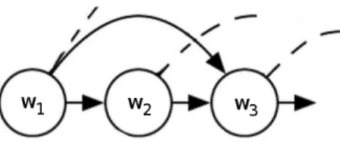
5 Example of Skip-Gram model as a probabilistic directed graphical model. Condi-tioned on word w2 the model aims to predict the surrounding words: w1, w3, w4

and so on. The dashed lines indicate arrows to words outside the diagram. . . 17

6 Illustration of the Skip-Thought Vectors model. Illustration taken from Kiros et al. (2015, p. 2) . . . 18

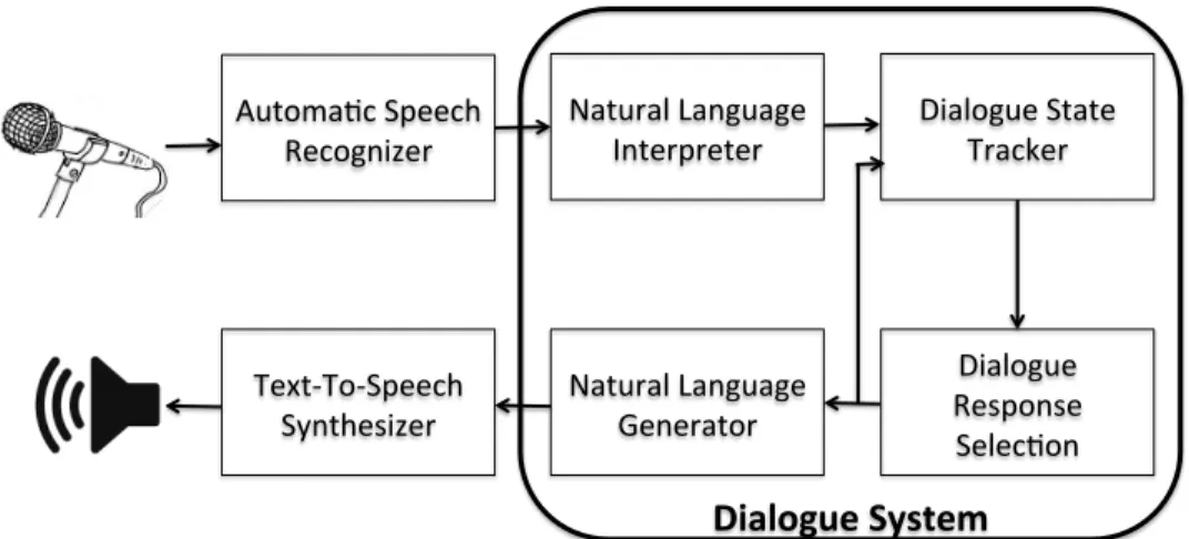
7 An overview of components in a dialogue system, reproduced from Serban et al. (2018). . . 30

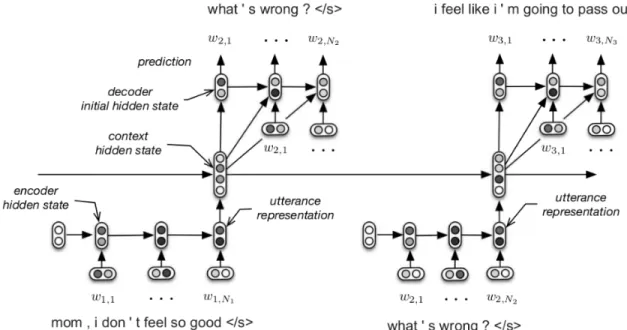
8 The computational graph of the HRED architecture for a dialogue composed of three turns. Each utterance is encoded into a dense vector and then mapped into the dialogue context, which is used to decode (generate) the tokens in the next utterance. The encoder RNN encodes the tokens appearing within the utterance. The context RNN encodes the discourse-level context of the utterances appearing so far in the dialogue, allowing information and gradients to flow over longer time spans. The decoder predicts one token at a time using a RNN. This figure was adapted from Sordoni et al. (2015a). . . 38

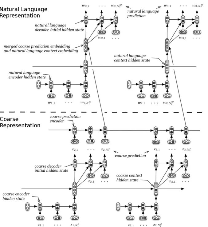
9 Computational graph for the Multiresolution Recurrent Neural Network (MrRNN). The lower part models the stochastic process over coarse tokens, and the upper part models the stochastic process over natural language tokens. The rounded boxes represent (deterministic) real-valued vectors, and the variables z and w represent the coarse tokens and natural language tokens respectively. . . 45

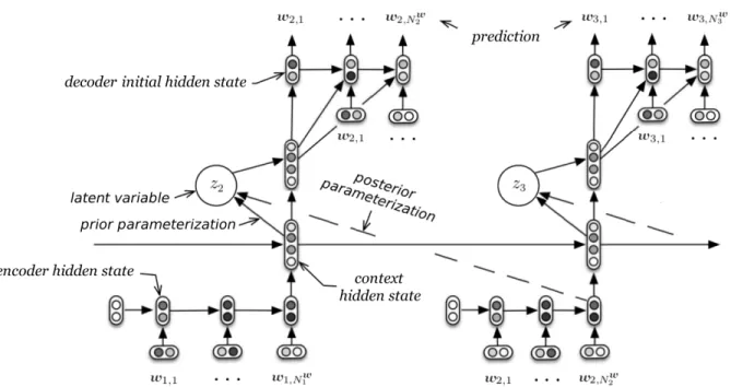
10 Computational graph for VHRED model. Rounded boxes represent (deterministic) real-valued vectors. Variables z represent latent stochastic variables. . . . 48

(16)

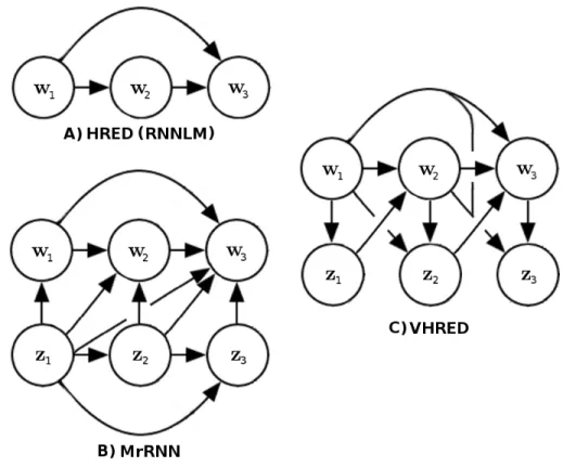
11 Probabilistic graphical models for dialogue response generation. Variables w rep-resent natural language utterances. Variables z reprep-resent discrete or continuous stochastic latent variables. (A): HRED (and RNNLM) uses a shallow generation process. This is problematic because it has no mechanism for incorporating uncer-tainty and ambiguity at a higher level, and because it forces the model to gener-ate compositional and long-term structure incrementally on a word-by-word basis. (B): MrRNN expands the generation process by adding a sequence of observed, discrete stochastic variables for each utterance, which helps generate responses with higher level semantic structure. (C): VHRED expands the generation process by adding one learned latent variable for each utterance, which helps incorporate uncertainty and ambiguity in the representations and generate meaningful, diverse responses. . . 51

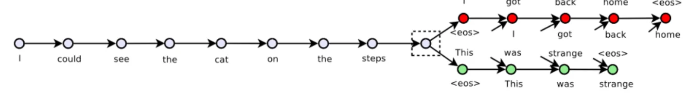
12 Screenshot of one dialogue context with two candidate responses, which human evaluators were asked to choose between. . . 60

13 Probabilistic directed graphical model for Latent Variable Recurrent Encoder-Decoder RNN with stochastic latent dynamics. . . 68

14 Probabilistic directed graphical model for Latent Variable Recurrent Encoder-Decoder RNN with deep stochastic latent dynamics. . . 70

15 Dialogue manager control flow. . . 79

16 Computational graph for the scoring models, used for the response selection poli-cies based on both state-action-value function and stochastic policy parametriza-tions. Each model consists of an input layer with 1458 features, a hidden layer with 500 hidden units, a hidden layer with 20 hidden units, a softmax layer with 5 output probabilities, and a scalar-valued output layer. The dashed arrow indicates a skip connection (the last hidden layer output is passed to the last output layer through an affine linear function). . . 85

17 Amazon Mechanical Turk (AMT) class frequencies on the AMT test dataset w.r.t. candidate responses selected by different policies. . . 91

18 Probabilistic directed graphical model for the Bottleneck Simulator. For each time step t, zt is a discrete random variable which represents the abstract state of the

dialogue, strepresents the dialogue history (i.e. the state of the agent), atrepresents

the action taken by the system (i.e. the selected response), ytrepresents the sampled

(17)

19 Contingency table comparing selected response models between Supervised AMT and Bottleneck Simulator. The cells in the matrix show the number of times the Supervised AMT policy selected the row response model and the Bottleneck Simulator policy selected the column response model. The cell frequencies were computed by simulating 500 episodes under the Bottleneck Simulator environment model. Further, it should be noted that all models retrieving responses from Reddit

have been agglomerated into the class Reddit models. . . 110

20 Response model selection probabilities across response models for Supervised AMT, REINFORCE and Bottleneck Simulator on the AMT label test dataset. 95% confidence intervals are shown based on the Wilson score interval for binomial distributions. . . 111

21 Screenshot of the introduction (debriefing) of the experiment. . . 157

22 Screenshot of the introductory dialogue example. . . 158

23 Fluency and relevancy reference table presented to human evaluators. . . 159

24 Consent screen for Amazon Mechanical Turk human intelligence tasks (HITs). . . 173

25 Instructions screen for Amazon Mechanical Turk human intelligence tasks (HITs). 174 26 Annotation screen for Amazon Mechanical Turk human intelligence tasks (HITs). The dialogue text is a fictitious example. . . 175

(18)

V

Notation

• {·} denotes a set of items. • (·) denotes a sequence of items.

• {xi}Ii=1(or simply {xi}i) denotes a set of items x1, x2, . . . , xI−1, xI.

• |V |, where V is a set, is the cardinality of the set (for example, if V is a finite set, then |V | is the number of elements in the set).

• A × B = {(a, b) | a ∈ A, b ∈ B}, where A and B are sets of items, denotes the Cartesian product of A and B.

• R denotes the set of real-valued numbers.

• Rn_{denotes the set of real-valued numbers in n dimensions.}

• N denotes the set of non-negative integer numbers. • N+_{denotes the set of positive integer numbers.}

• N−_{denotes the set of negative integer numbers.}

• a ∈ R denotes a real-valued variable named a.

• [a, b], where a, b ∈ R and b > a, denotes the closed set of real-valued numbers between a and b, including a and b.

• (a, b), where a, b ∈ R and b > a, denotes the open set of real-valued numbers between a and

b, excluding a and b.

• a ∈ Rn_{denotes a real-valued vector of n dimensions.}

• A ∈ Rn×m_{denotes a real-valued matrix of n × m dimensions.}

• AT _{and A}T _{both denote the transpose of the matrix A.}

• i = 1, . . . , n means that i will take integer values 1, 2, 3, 4, 5 and so on until and including integer n.

• An n-gram is a sequence of n consecutive words (or tokens). • w ∈ U , where U is a sequence of tokens, denotes a token inside U .

(19)

• exp(x) and ex _{denotes the exponential function of the value x.}

• log(x) and ln(x) denotes the natural logarithm function of the value x. • tanh(x) denotes the hyperbolic tangent taken of value x.

• f0_{(x) denotes the derivative of the function f w.r.t. variable x.}

• δ

δxf (x) denotes the derivative of the function f w.r.t. variable x.

• ∇θfθ(x) denotes the derivative of the function f w.r.t. parameters θ. If θ is a vector, then it

denotes the Jacobian matrix.

• x · y, where x and y are vectors or matrices, denotes the element-wise product between x and y.

• x often denotes an input variable (e.g. a real-valued variable or an input sequence of string tokens).

• y often denotes an output variable (e.g. an output label, such as a user intention label). • θ and ˆθ usually denote model parameters.

• ψ and ˆψ usually denote model parameters.

• Pθ(·) usually denotes the probabilistic model parametrized by parameters θ.

• x ∼ Pθ(x) denotes a sample of the random variable x following the probabilistic model

parametrized by parameters θ.

• Nx(µ, Σ) denotes the probability of variable x under a multivariate normal distribution with mean µ and covariance matrix Σ.

• x ∼ Uniform(a, b) denotes that x is an integer random variable sampled at uniformly random from the set {a, a + 1, · · · , b − 1, b}, with a, b ∈ N and b > a.

• x ∼ Uniform(A), where A is a finite discrete set, denotes that x is a random variable sampled at uniformly random from the set A.

• Ex∼P (x)[f (x)] = PxP (x)f (x) =

R

P (x)f (x)dx is the expectation of the function f (x)

w.r.t. the random variable x following the distribution given by the probability or density function P .

(20)

• KL[Q||P ] = −R

Q(x) log(Q(x)/P (x))dx is the Kullback-Leibler (KL) divergence between

the two probability distributions P (x) and Q(x).

• 1(·)denotes a Dirac-delta function, which equals one if the statement (·) is true, and

other-wise equals zero.

• ∀ denotes the for all operator.

(21)

VI

Acknowledgements

I had no idea of what I had commited myself to when I decided to study for a Ph.D. degree. I made this decision while I was still studying my master’s degree at University College London (UCL). Back then, my future supervisor Yoshua Bengio had come to UCL to give a talk about some of the advances of deep learning. Although I did not understand much of the talk, I found the abstract ideas he presented facinating and I thought it was a pity that they were not covered in more depth in any of my courses at the time. After his talk, another student and I had a chance to chat with him about his research and about machine learning in general. As the discussion turned to the topic of future research and the many real-world applications of our field, I saw a spark in his eyes and I realized that this was someone I wanted to work with. Afterwards, I went home and discovered that I had, in fact, already read and cited several of his older papers in my bachelor’s thesis. It was at this point that I decided to apply for studying a Ph.D. degree in his research lab.

I was accepted into the Ph.D. program, and the following fall I arrived in Montreal. This was at once both a very exciting and a frightening time. I had never been to Canada before, I did not know anyone there and I certainly wasn’t prepared for the language barrier or the harsh weather to come. Fortunately, the professors and students in the lab were very welcoming and helpful. It turned out that, like myself, many of them had come from abroad. This was when I got to know Aaron Courville, my second supervisor. I quickly realized that he was one of the people I could communicate with most easily. Every time one of us explained a complex idea, it seemed as if the other one instantly understood it and started extending it. I also found out that we shared many of the same ideas about probabilistic graphical models and their uses in deep learning models. I was fortunate enough that Aaron had time available and could take me on as one of his students. Through discussions with Yoshua and Aaron, I decided to focus my research on the application of deep learning and reinforcement learning for building dialogue systems. Shortly after, I was introduced to Joelle Pineau, my future unofficial advisor and long-term collaborator. Joelle had previously worked on applying reinforcement learning for building dialogue systems, and she was keen to start a new research group focused on it. A few months later, we started a research group with other students investigating deep learning and reinforcement learning techniques for building dialogue systems. This research group was of great help, because its weekly meetings provided a common structure and framework for us to work together. That is how the journey of my Ph.D. began nearly 5 years ago, with the help and supervision of Yoshua, Aaron and Joelle. I’d like to thank each of them for their enduring help and support throughout the years. Without them, my Ph.D. degree would never have been possible.

When I started, I thought that a Ph.D. mainly involved reading papers, running experiments and then writing papers: a set of well-defined, repeatable steps aimed towards advancing scientific

(22)

knowledge bit by bit. Although this is certainly part of it, I later discovered that a Ph.D. is also a long journey of exploration, discovery and reflection. It is a meticulous process of asking questions and seeking answers, where both the questions and answers are always kept under scrutiny. This process involves learning the assumptions and general world view of the researchers in the field and questioning them, as well as learning the general methodology of the field (including how to set up experiments, use software libraries, write scientific papers, and so on). However, the pro-cess also demands patience, persistence, diligence and last, but not least, a will to go on solitary campaigns to promote new ideas, ask new questions and give new answers. For accompanying me along this long and difficult journey, I would like to thank all of my collaborators who I have worked with throughout the years, including students and university staff members at University of Montreal and McGill University. In particular, I would like to thank Alessandro Sordoni, Caglar Gulcehre and Laurent Charlin, who have been supportive and who have helped teach and mentor me throughout the years. I would also like to give particular thanks to students in the dialogue research group: Nicolas Angelard-Gontier, Peter Henderson, Ryan Lowe, Michael Noseworthy, Prasanna Parthasarathi, Nissan Pow and Koustuv Sinha. Without their feedback and brainstorming meetings, many of the ideas proposed in this thesis would never habe been possible. I would also like to thank our team members from the Amazon Alexa Prize 2017 competition: Chinnadhurai Sankar, Mathieu Germain, Saizheng Zhang, Zhouhan Lin, Sandeep Subramanian, Taesup Kim, Michael Pieper, Sarath Chandar, Nan Rosemary Ke, Sai Rajeswar, Alexandre de Brebisson, Jose M. R. Sotelo, Dendi Suhubdy, Vincent Michalski and Alexandre Nguyen. Although we did not win the competition, I am very proud to have worked together with them. Even though our work together is not covered in this thesis, I also had fruitful collaborations with Sungjin Ahn, Sarath Chandar, Alberto Garcia-Duran, Caglar Gulcehre and Alexander G. Ororbia II over the past few years. I am thankful to each of them for their collaboration and time. I would also like to thank all other team members of the Quebec Artificial Intelligence Institute (Mila), including in particular Hugo Larochelle, Frederic Bastien, Pascal Lamblin and Arnaud Bergeron for their help and tech-nical assistance. I would also like to thank my collaborators from IBM Research: Tim Klinger, Kartik Talamadupula, Gerald Tesauro and Bowen Zhou. I hope our paths will cross again in the future. Last, not but not least, I would like to thank the thesis jury members for reading my thesis and providing their comments: Alain Tapp, Pascal Vincent, Aaron Courville, Yoshua Bengio and Phil Blunsom.

(23)

Finally, and most of all, I would like to thank my love, my wife and partner in life, Ansona Onyi Ching and our son Octavian Ching Serban. Ansona has stood by my side throughout the years, since before I started studying my Ph.D. degree, and she has always helped me shoulder the inevitable ups and downs of the journey. Much of my inspiration and courage to move forward with bold decisions and ideas has come from her. Octavian has in turn given the two of us a life of happiness and purpose, which I am not sure could be matched by any amount of scientific achievement. None of this would have been possible without their love and support.

(24)

1 Introduction

1.1 Motivation

Over the past decades, computers have become a ubiquitous and essential part of modern society. As a part of this transformation, the way we interact with computers has changed tremendously. The computers in the middle of the 20th century could only be programmed manually by swapping in different punch cards. Later, computers were equipped with an extensive internal memory and could be programmed by interacting with a terminal using a keyboard. In the 80s, a new wave of computers, known as personal computers, started to appear with graphical user interfaces, which allowed users to more naturally interact with them using both mouse and keyboard devices. Since then, other types of computers have emerged, including mobile smartphones, tablet computers and GPS navigation devices, which can be interacted with using touch gestures (e.g. touch user interfaces), as well as virtual reality platforms and the XBox 360 (Kinect), which can be interacted with using head and body gestures. Since at least the 90s, automated telephone systems (called spoken dialogue systems) have also been developed, which could understand natural language speech, for example by AT&T Research Labs. However, these systems were often exclusively built for one particular task with extremely limited capabilities, compared to the general interfaces discussed earlier. The reader is likely familiar with all of these technologies, but highlighting the chronological development of these technologies and their transformations serve an important purpose. With each new transformation computer interfaces have become more intelligent and more natural to interact with.

Very recently, software companies (e.g. Apple, Microsoft, Google, Amazon and Nuance) have started to develop general natural language dialogue systems, called intelligent personal assistants. These personal assistants aim to bridge one of the ultimate communication gaps between humans and computers, by allowing humans to interact with computers directly using spoken natural lan-guage for carrying out a multitude of tasks. Unfortunately, understanding and generating natural language is a very difficult problem. Therefore, it is not surprising that these technologies are still in their very infancy. This thesis is motivated by these technological developments and the related outstanding challenges. In addition to intelligent personal assistants, dialogue systems have also been deployed as supportive virtual friends (Markoff and Mozur, 2015;Dillet, 2016), healthcare assistants (Furness,2016;Brodwin,2018) and tutoring assistants (Nye et al.,2014).

The purpose of this thesis is to make a contribution to the research fields of natural language processing and representation learning, with the specific aim of building general-purpose natural language dialogue systems. In particular, the thesis will focus on probabilistic generative models for building natural language dialogue systems using large text corpora.

(25)

1.2 Central Assumptions

As is the case with much of scientific research, the work in this thesis is built upon several key assumptions. These key assumptions constitute the foundations underlying and motivating the work presented in this thesis. Some of these assumptions are well-established in the field, while others might be more contestable. This section provides an overview and discussion of these assumptions.

The first key assumption of this thesis is that communication between humans and machines should be collaborative in nature and be beneficial to all parties. In any conversation, both the human interlocutors (human speakers) and the machine interlocutors (machine speakers) are agents in their own respect, each one with their own goals. The reason that any two interlocutors might have a conversation in the first place must be because they both believe that there is something to be gained through the conversation. In other words, each interlocutor believes that there exists an alignment between their own goals and the goals of the other party, and that by conducting a conversation they may both benefit from it. However, it is important to stress that their goals are not necessarily perfectly aligned. Let’s consider the example of a dialogue system selling flight tickets. In addition to its primary goal of finding a suitable ticket for a human customer, the system may have a secondary goal to maximize profits by selling the most expensive ticket commensurate with the human customer’s spending budget. This secondary goal would be in direct conflict with the human customer, if the human customer has a secondary goal of purchasing an inexpensive ticket.

The second key assumption is that, in general, the human and machine interlocutors only have access to partial information about the state of the world, about the other interlocutor’s information and goals and even about their own goals. For example, the dialogue system selling flight tickets cannot know the goals of a human customer beforehand, such as their departure city, destination city or even their spending budget. On the other hand, the human customer does not know which flight tickets are available and at what prices. The human customer may not even know their destination city or their exact spending budget. This is something the human customer might decide on based on the options presented by the dialogue system (e.g. based on the available destination cities and the price differences between economy and business class shown by the dialogue system).

Although these two key assumptions may appear evident to the avid reader, they go against some of the assumptions implied by some of the literature on goal-driven dialogue systems. In particular, research on voice control systems (or voice command systems) has sometimes made the implicit assumption that a goal-driven dialogue system should serve as a direct substitute for key-board input, which will convert the human interlocutor’s speech to an appropriate query and submit

(26)

it to an application or a service API. For example, consider the case of a voice-controlled GPS-based navigation system. This system might only expect the human user to mention a destination (e.g. an address or a location name) and would then, based on the received destination, map out a route for the human user and display it in a graphical user interface. Strictly speaking, this is not a collaborative dialogue where both parties stand to benefit. Rather it is a one-way communication channel, where the system’s main purpose is to convert the words spoken by the human user into an appropriate format (e.g. an address string represented in a formal language) for making a query to a subsequent application or service. This is an example of semantic parsing (Wilks and Fass,

1992;Kamath and Das,2019)

This simple system further makes the assumption that the human user has access to all relevant information, including their own goal (e.g. the exact destination address and the format the system requires).

The previous two assumptions discussed were related to the form of communication between the human and machine interlocutors. The next set of assumptions is related to the building of dialogue systems. A key assumption here is that versatile dialogue systems, which both satisfy the previous assumptions and are capable of solving real-world problems through effective and natural interactions with humans, can only be built by incorporating data-driven approaches. Such dialogue systems must incorporate modules based on data-driven approaches, such as machine learning, in order to solve either all or a subset of the underlying engineering problems (for ex-ample, natural language understanding, natural language generation and general decision making). This assumption has been adopted widely by the dialogue system research community, as will be discussed below. However, it should be noted how this assumption stands in contrast to predomi-nantly rule-based dialogue systems (such as the ELIZA system and the ALICE system discussed later). Nevertheless, this assumption seems reasonable given the complexity of many of the under-lying engineering problems. Consider, for example, the natural language understanding problem of classifying the intention of spoken utterances. Given the magnitude of possible intentions, the diversity of ways in which each intention can be formulated, and finally the contextual, ambiguous and error-prone nature of natural language, it would seem extremely difficult to build a determin-istic, rule-based system to map any utterance to its underlying intention.

This thesis focuses on building dialogue systems using deep learning (a branch of machine learning), which is particularly suitable for large-scale data-driven machine learning. As will be discussed later on, the field of deep learning has made tremendous advances and helped set new state-of-the-art performance records across a variety of natural language processing tasks over the past few years. Many of the advances of deep learning have helped with natural language represen-tations (e.g. methods for representing words, phrases and sentences) and natural language genera-tion (e.g. generating phrases and sentences condigenera-tioned on specific informagenera-tion), which constitute

(27)

sub-problems faced by most dialogue systems. This makes deep learning particularly relevant for research on building general-purpose natural language dialogue systems.

The final key assumption of this thesis is based on the premise that humans learn about the world and about how to communicate through natural language by observing and interacting with others. For example, a toddler might hear a word spoken by a parent and then learn to associate that word with a particular object in the world. As a more elaborate example, consider a student studying deep learning, who is in the process of implementing a machine learning model. She might search on the Internet for similar implementations and find a relevant discussion thread on a forum website (such as Reddit or Stack Overflow). Suppose that on this discussion thread, another person exposes a solution to a similar problem and receives feedback from others about missing aspects in the implementation. By reading through the discussion thread, our protagonist might learn about the subtasks involved in her own implementation. Using this information, she might decompose the task into subtasks, with which she is already familiar, and finalize her own implementation. Alternatively, she may seek additional help by asking a related question in the discussion thread. Although our premise is that humans learn a significant amount of knowledge about the world and about how to communicate by observing and interacting, the reader should note that the premise is not that all knowledge is learned or acquired through these mechanisms. A significant amount of learning is bound to also occur through other mechanisms (for example, observing others do a task and then imitating it without any two-way communication). The premise is only that a significant amount of information is being learned by observing and interacting with others, and that this is a valuable source of information in its own right.

By accepting this premise – that humans learn a significant amount about the world and about how to communicate by observing others and by interacting with others – we arrive at the final key assumption of this thesis. The assumption is that a machine can also learn a significant amount of information about the world and about how to communicate in natural language by observing and interacting with others. This last assumption is perhaps the most contestable of all the assumptions discussed so far. However, it may be mitigated if it is further assumed that the system has access to other information, such as knowledge bases and encyclopedias.

Unfortunately, it is difficult to deploy real-world machine learning systems and, often even more difficult, to entice human users to interact with such systems and to collect relevant interaction data. Therefore, in the first part of this thesis, we will restrict the last assumption even further. Specifically, we will assume that a significant amount of information about the world and about how to communicate can be learned by simply observing the interactions of others (e.g. interactions between human interlocutors). In other words, by giving a machine access to a corpus or a stream of data containing interactions between human interlocutors, the machine can learn a substantial amount of information about the real world and about how to communicate in natural language.

(28)

This most restrictive version of the last assumption poses a problem for the so-called grounding process of natural language (Harnad,1990;Quine, 2013). Without going into further details, one part of this process is where a learner learns to associate linguistic expressions with their mean-ings, such as words and their intended referents. This is very difficult to accomplish without any additional information. Consider the thought experiment presented byHarnad(1990): “Suppose you had to learn Chinese as a second language and the only source of information you had was a Chinese/Chinese dictionary. The trip through the dictionary would amount to a merry-go-round, passing endlessly from one meaningless symbol or symbol-string to another, never coming to a halt on what anything meant.”. This thought experiment is very similar to the most restrictive version of our last assumption, where the system has to learn the meaning of words, phrases, dialogue turns and entire interactions by only observing the conversations between third-party interlocutors. However, in our case, the system has access to more information than inHarnad(1990)’s thought experiment. The system observes the interactions between interlocutors and can identify and dis-tinguish the different interlocutors. As a minimum, the observed phrases can be grounded by the interlocutor who spoke them. In addition, the system knows that the dialogues are collaborative in nature, and that the majority of dialogues are beneficial to each party and involve some form of information exchange. Given this additional knowledge about each conversation, the system may be able to ground more of the linguistic content. For example, phrases emitted by one interlocutor, but not by another interlocutor, might be grounded as a “goal statement” or as an “information ex-change” since such phrases must be present in the dialogue and would often only be spoken by one interlocutor.1 _{Naturally, the process of grounding natural language becomes easier if the system}

has access to other information (e.g. knowledge bases, encyclopedias) or if the system can interact with human users. This is the case for the second part of the thesis.

1.3 Thesis Structure

The thesis is structured as follows.

Chapter 2 covers background theory related to machine learning and dialogue systems. The chapter is split into three parts. The first part focuses on probabilistic generative models, which form the foundation and act as a unifying framework for much of the work presented in this thesis. Neural network models are also presented here. The second part introduces reinforcement learning, a set of techniques used extensively later in the thesis. The third part discusses dialogue systems in detail, including system components, methods for optimizing system components and methods for system evaluation.

Chapter 3 proposes three sequence-to-sequence models, a class of generative deep neural

(29)

works, for building generative dialogue models. Given a sequence of turns from a text-based dialogue, these models aim to generate an appropriate next response in the dialogue. The three models proposed are the Hierarchical Recurrent Encoder-Decoder (HRED), Multiresolution Re-current Neural Network (MrRNN) and Latent Variable ReRe-current Encoder-Decoder (VHRED). For each model, the contribution of the author of this thesis, the motivation, the prior related work and the model architecture and corresponding learning algorithm are discussed. Following this, experi-ments are presented on two dialogue response generation tasks: a Twitter response generation task and a Ubuntu technical response generation task. The chapter concludes with a general discussion and directions for future research.

Chapter 4 investigates a framework for building dialogue systems, based on combining rep-resentation learning and reinforcement learning, in order to develop a non-goal-driven dialogue system capable of learning from real-world interactions with humans. The work presented here focuses on the Milabot system built by the Quebec Artificial Intelligence Institute (Mila) for the Amazon Alexa Prize 2017 competition. The chapter first discusses the contribution of the author of this thesis. The chapter then discusses the motivation of the new framework and compares it to the earlier task of building generative dialogue models. Following this, a review of prior related work is presented. Then, the chapter presents an overview of the Milabot system and its underly-ing ensemble system, which consists of models generatunderly-ing natural language system responses. The problem of selecting an appropriate system response is presented next and framed as a sequential decision making problem, motivated by reinforcement learning methods. Following this, several reinforcement learning algorithms and supervised learning algorithms are proposed in order to learn policies capable of selecting an appropriate system response. In particular, a model-based reinforcement learning algorithm, named the Bottleneck Simulator, is proposed. Then, the chap-ter presents experiments evaluating the proposed policies, conducted based on real-world users, crowdsourced human annotations and simulations. Finally, the chapter concludes with a broader discussion and directions for future research.

Chapter 5 concludes the thesis. The chapter provides a brief summary of the work carried out in the thesis, reviews the main conclusions and provides a bird’s-eye view of the work from the perspective of probabilistic generative models.

(30)

2 Technical Background

2.1 Probabilistic Generative Models

This thesis focuses on the field known as machine learning, a sub-field of computer science, statis-tics and mathemastatis-tics (Bishop, 2006; Goodfellow et al., 2016). This chapter will introduce the technical background required to understand the reminder of the thesis and also provide pointers for further reading.

Arthur Lee Samuel defined the machine learning field as follows: "[A field] of study that gives computers the ability to learn without being explicitly programmed" (Simon, 2013). In this sen-tence, Samuel highlights precisely the advantage of machine learning for solving natural language generation and understanding problems. It is humanly impossible to explicitly write down rules for understanding and generating every relevant sentence for every conceivable natural language pro-cessing task. Therefore, it is necessary to build a computer with the ability to learn without being explicitly programmed. This is often done by letting a computer program learn from examples.

In the following, we will assume that the reader is familiar with basic calculus and probability theory, including concepts such as integrals, linear algebra, random variables, probability distribu-tions, expectadistribu-tions, probabilistic independence and so on. In case the reader is not familiar with this material, please refer toFriedman et al.(2001) andBishop(2006) for a detailed introduction to all of these. As another reference, the reader may also refer toGoodfellow et al.(2016).

The first concept we introduce is the probabilistic directed graphical model. A probabilistic directed graphical model is a set of random variables x = {xm}Mm=1 and an associated directed

graph G = {{xm}Mm=1, {ei}Ii=1}, with vertices (nodes) xm, for m = 1, . . . , M , and edges ei, for

i = 1, . . . , I. The nodes are random variables. Each edge e ∈ G has a tail, which corresponds to

its origin node and a head, which corresponds to the node it is pointing to (different from the origin node). We define Pa(xm) as the set of parents of the random variable xm, where xj ∈ Pa(xm)

if there exists an edge with tail xj and head xm. The graph G must then satisfy the following

factorization of the distribution over x:

P (x) =

M

Y

m=1

p(xm|Pa(xm)). (1)

This factorization is crucial for understanding the relationships between the random variables. Given a probabilistic directed graphical model, we are able to follow the generative process of the model as well as deduce independence statements about the underlying random variables (Bishop,

2006). To illustrate this, take the directed graphical model shown in Figure1as an example. This model has random variables x1, x2, x3, which according to the edges can be factorized as follows:

(31)

Based on this factorization, we may deduce that x1 ⊥⊥ x2, i.e. that x1 is unconditionally

indepen-dent of x2. We arrive at this result by integrating out x3:

P (x1.x2) = Z P (x1, x2, x3)dx3 = Z P (x1)P (x2)P (x3|x1, x2)dx3 = P (x1)P (x2) Z P (x3|x1, x2)dx3 = P (x1)P (x2)

Importantly we always assume that the probabilistic directed graphical model be non-acyclic.

Figure 1: Example of a probabilistic directed graphical model.

In other words, there cannot exist any directed paths (sequence of connected edges) starting and ending at the same node.

2.1.1 n-Gram Models

An important class of probabilistic models are the n-gram models for discrete sequences, where

n ∈ N and where N denotes the set of positive integers. Let w = (w1, . . . , wM) be a sequence

of M discrete symbols, where wm ∈ V for discrete set V . For example, the variables may be the

words of a natural language dialogue or the words of a web document, represented by their indices. The n-gram model, with parameters θ, assumes the distribution over variables factorizes:

Pθ(w) = Pθ(w1, . . . , wM) = Pθ(w1)Pθ(w2|w1) · · · Pθ(wn−1|w1, . . . , wn−2) M Y m=n Pθ(wm|wm−n+1, . . . , wm−1)

The key approximation is that the probabilities over each variable can be computed using only the previous n − 1 tokens:

P (wm|w1, . . . , wm−1) ≈ Pθ(wm|wm−n+1, . . . , wm−1)

(32)

where θv,wm−n+1,...,wm−1 ∈ [0, 1] is the probability of observing token v given the n − 1 previous

tokens wm−n+1, . . . , wm−1, which must sum to one: Pv∈V θv,wm−n+1,...,wm−1 = 1. For the 2-gram

model, also known as the bigram model, the factorization corresponds to the directed graphical model shown in Figure 2. This model is a probabilistic generative model, since it can assign a probability to any sequence of variables w1, . . . , wM and since it can generate any such sequence

by sampling one variable at a time (first sampling w1, then sampling w2 conditioned on w1 and so

on). This model is used widely in natural language processing applications (Goodman,2001).

Figure 2: Probabilistic graphical model for bigram (2-gram) model. Let {wi}I

i=1 be a set of I example sequences, called the training dataset. We assume that the

example sequences are independent and identically distributed. The model parameters θ may be estimated (learned) by maximizing the log-likelihood on the training set:

θ = arg max

θ0

X

i

log Pθ0(wi).

This is done by setting θv,wm−n+1,...,wm−1 to be proportional to the number of times token v was

observed after tokens wm−n+1, . . . , wm−1 in the training set. In practice, the parameters are often

normally regularised or learned with Bayesian approaches (Goodman,2001).

The approximation discussed earlier is problematic. As n grows, the model begins to suffer from what is known as the curse of dimensionality (Richard, 1961; Bishop, 2006). Since the variables are discrete, the number of possible combinations of n variables is |V |n, which grows exponentially with n. This means that to estimate parameters θ, the model requires a number of data examples exponential in n. Therefore, in practice, n is usually a small number such as 3 or 4.

2.1.2 Recurrent Neural Networks

The second class of models we consider are known as recurrent neural networks (RNNs). We will focus on the well-established recurrent neural network language model (RNNLM) (Mikolov et al., 2010; Bengio et al., 2003). Other variants have been applied to diverse sequential tasks, including speech synthesis (Chung et al.,2015), handwriting generation (Graves,2013) and music composition (Boulanger-Lewandowski et al., 2012; Eck and Schmidhuber, 2002). As before, let

w1, . . . , wM be a sequence of discrete variables, such that wm ∈ V for a set V . We shall call V

(33)

model, with parameters θ, which decomposes the probability over tokens: Pθ(w1, . . . , wM) = M Y m=1 Pθ(wm|w1, . . . , wm−1). (2)

Unlike the n-gram models, the RNNLM does not make a hard assumption restricting the distri-bution over a token to only depend on the n − 1 previous tokens. Instead, it parametrizes the conditional output distribution over tokens as:

Pθ(wm+1 = v|w1, . . . , wm) = exp(g(hm, v)) P v0_∈V exp(g(h_m, v0)) , (3) g(hm, v) = OvThm, (4) hm = f (hm−1, Iwm), (5)

where hm ∈ Rdh, for m = 1, . . . , M , are real-valued vectors called hidden states with

dimensional-ity dh ∈ N. The function f is a non-linear smooth function called the hidden state update function.

For each time step (each token) it combines the previous hidden state hm−1 with the current token

input wm to output the current hidden state hm. The hidden state hm acts as summary of all the

tokens observed so far, which effectively makes it a sufficient statistic from a statistical point of view. The matrix I ∈ Rde×|V | _{is the input word embedding matrix, where column j contains the}

embedding for word (token) index j and de ∈ N is called the word embedding dimensionality.

Similarly, the matrix O ∈ Rde×|V | _{is called the output word embedding matrix. By eq. (}₃_{) and}

eq. (4), the probability distribution over token wm+1 is parametrized as a softmax function over

the dot products between the hidden state and the output word embeddings for each word in the vocabulary. Therefore, the more similar an output word embedding vector Ovis to the hidden state

vector hm (e.g. the smaller the angle between the two vectors) the higher the probability assigned

to token v.

Unlike the n-gram models discussed earlier, the RNNLM does not parametrize a separate prob-ability value for every possible combination of tokens. Instead it embeds words into real-valued vectors using the word embedding matrices, thereby allowing the rest of the model to use the same set of parameters for all words observed. This was the key innovation behind the so-called neural network language model proposed by Bengio et al.(2003), and it is used by the RNNLM and its extensions, which gained state-of-the-art performance on several machine learning tasks (Mikolov et al., 2010;Jozefowicz et al., 2016; Devlin et al., 2018). In addition to this, by using a RNN to compute the hidden state which parametrizes the output distribution, the RNNLM can potentially capture an unlimited amount of context (unlike both n-gram models and the earlier neural network language models). This is also the main motivation for the generative models we will discuss later. The graphical model is illustrated in Figure3.2

(34)

Figure 3: Probabilistic graphical model for a recurrent neural network language (RNNLM) model. The model parameters are learned by maximum likelihood. However, unlike the n-gram mod-els discussed earlier, there exists no closed-form solution. Therefore, the parameters are usually learned using stochastic gradient descent on the training set. Let {wi_}I

i=1be the training dataset.

An example sequence wi _{is sampled at random, and the parameters are updated:}

θ ← θ + α∇θlog Pθ(w1i, . . . , w i Mi),

where α > 0 is the learning rate and Mi is the length of sequence i. In practice, any first-order

optimization method can be used. For example, the method Adam developed byKingma and Ba

(2015) tends to work well and it is therefore used in all experiments presented in the first part of this thesis. For large models, in practice, the gradient w.r.t. each parameter can be computed efficiently using graphics processing units (GPUs) and parallel computing in combination with the backpropagation algorithm, a type of dynamic programming (Goodfellow et al.,2016).

There exists different parametrizations of the function f . One of the simplest and most popular parametrizations is the hyperbolic tangent one-layer neural network:

f (hm−1, Iwm) = tanh(H

i_I

wm + Hhm−1), (6)

where H ∈ Rdh×dh _{and H}i ∈ Rdh×de _{are its parameters. Usually a constant, called the bias or}

intercept, is also added before applying the hyperbolic tangent transformation, but to keep the notation simple we will omit this. Another popular variant is the Gated Recurrent Unit (GRU) proposed byCho et al.(2014):

rm= σ(Iwrm+ Hrhm−1), (reset gate) (7)

um= σ(Iwum+ Huhm−1), (update gate) (8)

¯

hm= tanh(HiIwm+ H(rm· hm−1)), (candidate update) (9)

hm= (1 − um) · hm−1+ um· ¯hm, (update), (10)

where · is the element-wise product and σ is the element-wise logistic function:

σ(x) = 1

1 + exp(−x), (11)

(35)

and where I, Ir, Iu _{∈ R}dh×|V |_{, H, H}

r, Hu ∈ Rdh×dh and Hi ∈ Rdh×de are the parameters. The

motivation for this parametrization is that the reset gate and update gate equations control whether or not the model reuses the previous hidden state when computing the current hidden state. If the previous state is useless (i.e. its value will not help determine future tokens in the sequence), rm

should be close to zero and the candidate update will be based mainly on the current input wm.

If the previous state is useful (i.e. hm−1 may help predict future tokens in the sequence) then rm

should not be zero. If the previous state hm−1 is useful, but the current input is useless, then the

update gate should set um to zero ensuring that minimal information is stored from the current

input. In fact, when um is close to zero the update is linear and this helps propagate the gradients

in the training procedure. This parametrization appears to be superior to the hyperbolic tangent one-layer neural network across several machine learning problems (Greff et al., 2017). A third, also very popular, parametrization is the Long-Term Short-Term Unit (LSTM) (Hochreiter and Schmidhuber,1997): im = σ(Iwrm+ H ih_h m−1+ Hiccm−1), (12) fm = σ(Iwfm+ H f h_h m−1+ Hf ccm−1), (13) cm = fmcm−1+ imtanh(Iwcm+ H ch_h m−1), (14) om = σ(Iwom+ H oh_h m−1+ Hoccm), (15) hm = omtanh(cm), (16)

where hm, cm ∈ Rdh, for m = 1, . . . , M , are real-valued vectors, Ir, If, Ic, Io ∈ Rdh×|V | and

Hih_{, H}ic_{, H}f h_{, H}f c_{, H}ch_{, H}oh_{, H}oc_{∈ R}dh×dh _{are the parameters. The variables c}

m and hmcan be

folded into a single vector by concatenation and rewritten as a hidden state update function. The motivation behind the LSTM parametrization is similar to that of the GRU parametrization. In practice, the LSTM unit appears to yield slightly more stable training compared to the GRU unit, although in terms of performance they appear to perform equally well (Greff et al., 2017). For more details, the reader may also refer toLipton et al.(2015).

2.1.3 Latent Variable Models

Many probabilistic graphical models also contain latent (hidden) stochastic variables, i.e. stochas-tic variables which are not observed in the actual data. Two important classes of such models are the hidden Markov models (HMMs) and Kalman filters (also known as linear state space models). These models posit that there exists a sequence of latent stochastic variables, with precisely one latent stochastic variable for each observed token, which explains all the dependencies (e.g. corre-lations) between the observed tokens. Importantly, the latent stochastic variables obey the Markov property: each latent stochastic variable depends only on the previous latent stochastic variable.

(36)

This is similar to the bigram model discussed earlier. It is instructive to understanding the HMM and Kalman filter, as well as the role that latent variables may play in probabilistic graphical mod-els. Therefore, we continue by giving a formal definition for these two modmod-els.

As before, let w1, . . . , wM be a sequence of discrete variables, such that wm ∈ Vw for m =

1, . . . , M for a vocabulary Vw. Let s1, . . . , sM be a sequence of discrete latent variables, such that

sm ∈ Vs for m = 1, . . . , M for a discrete set Vs. The HMM, with parameters θ, factorizes the

probability over variables as:

Pθ(w1, . . . , wM, s1, . . . , sM) = Pθ(s1) M Y m=2 Pθ(sm|sm−1) M Y m=1 Pθ(wm|sm), (17) = θ_s0₁ M Y m=2 θs_s_m_,s_m−1 M Y m=1 θ_ww_m_,s_m, (18)

where θ0 _{∈ R}|Vs|, θs _{∈ R}|Vs|×|Vs|and θw _{∈ R}|Vw|×|Vs| are non-negative parameters, which define probability distributions. The corresponding graphical model is shown in Figure4. It is straight-forward to derive that the observed tokens are independent conditioned on the latent variables:

wm ⊥⊥ wm0|s_m, . . . , s0

mfor m 0 _{6= m.}

Figure 4: Probabilistic graphical model for hidden Markov model and Kalman filter model. Next, we describe a variant of the Kalman filter, where the observed sequence is discrete. Let w1, . . . , wM be a sequence of discrete variables, such that wm ∈ Vw for m = 1, . . . , M

for a vocabulary Vw. Let s1, . . . , sM be a sequence of continuous (real-world) latent variables,

distributed according to a normal distribution, such that sm ∈ Rdfor m = 1, . . . , M and d ∈ N.

The Kalman filter assumes that the latent stochastic variables define a trajectory in a continuous space, which describes the observations. The Kalman filter, with parameters θ, factorizes the probability over variables as:

Pθ(w1, . . . , wM, s1, . . . , sM) = Pθ(s1) M Y m=2 Pθ(sm|sm−1) M Y m=1 Pθ(wm|sm), (19) = Ns1(θ 0 µ, θ s Σ) M Y m=2 Nsm(θ s µsm−1, θsΣ) M Y m=1 exp(θw wm T_s m) P w0exp(θ_ww0Ts_m) (20)

(37)

where Nx(µ, Σ) is the probability of variable x under the multivariate normal distribution with mean µ ∈ Rdand covariance matrix Σ ∈ Rd×d. The parameters defining the generation process over latent stochastic variables are θ0_µ _{∈ R}d and θ_µs, θs_Σ _{∈ R}d×d. The parameter defining the generation process over observed variables is θw _{∈ R}d×|Vw|, used in a similar way to the RNN parameter in eq. (3). The graphical model is the same as the HMM model, shown in Figure4.

For the HMM, for small vocabularies Vs _{and V}w _{the model parameters may be learned}

us-ing the stochastic gradient descent procedure described earlier by simply summus-ing out the latent variables. For the Kalman filter, as well as the HMM with large vocabularies, the exact gradient updates are generally intractable and instead other procedures must be used. Two such training procedures are the expectation-maximization algorithm (EM), and the variational learning proce-dure (Friedman et al., 2001; Bishop, 2006). We will describe the variational learning procedure, since it will be used later in the thesis. The variational learning procedure assumes that a poste-rior distribution Qψ(s1, . . . , sM|w1, . . . , wM) is estimated, with parameters ψ, which approximates

Pθ(s1, . . . , sM|w1, . . . , wM) by a multivariate normal distribution. It utilizes a lower-bound on the

log-likelihood based on Jensen’s inequality: logPθ(w1, . . . , wM) = log X s1,...,sM Pθ(w1, . . . , wM, s1, . . . , sM) (21) = log X s1,...,sM Qψ(s1, . . . , sM|w1, . . . , wM) Pθ(w1, . . . , wM, s1, . . . , sM) Qψ(s1, . . . , sM|w1, . . . , wM) (22) ≥ X s1,...,sM Qψ(s1, . . . , sM|w1, . . . , wM) log Pθ(w1, . . . , wM, s1, . . . , sM) Qψ(s1, . . . , sM|w1, . . . , wM) ! (23) = X s1,...,sM Qψ(s1, . . . , sM|w1, . . . , wM) log Pθ(s1, . . . , sM)Pθ(w1, . . . , wM|s1, . . . , sM) Qψ(s1, . . . , sM|w1, . . . , wM) ! (24) = X s1,...,sM Qψ(s1, . . . , sM|w1, . . . , wM) log Pθ(w1, . . . , wM|s1, . . . , sM) − X s1,...,sM Qψ(s1, . . . , sM|w1, . . . , wM) log Qψ(s1, . . . , sM|w1, . . . , wM) Pθ(s1, . . . , sM) ! (25) = Es1,...,sM∼Qψ(s1,...,sM|w1,...,wM)[log Pθ(w1, . . . , wM|s1, . . . , sM)] − KL [Qψ(s1, . . . , sM|w1, . . . , wM)||Pθ(s1, . . . , sM)] , (26)

where Ex∼P(f (x)) is the expectation of function f (x), with x distributed according to P , and

KL[Q||P ] is the Kullback-Leibler divergence between distribution Q and P . The distribution

Qψ(s1, . . . , sM|w1, . . . , wM) depends on w1, . . . , wM. Given a set of data examples, it is

possi-ble to maintain a Q distribution with separate parameters ψ over each example. A popular variant of this approach is known as mean-field variational Bayes (Beal,2003). A more recent approach used in the neural network literature for continuous latent stochastic variables, is to have a neural