Activity induced variation in spin-orbit angles as derived from Rossiter-McLaughlin measurements

Astronomy & Astrophysics manuscript no. RM-VARIATION-ARXIV _{ESO 2018}c September 5, 2018

Activity induced variation in spin-orbit angles as derived from

Rossiter-McLaughlin measurements

?

M. Oshagh

, A. H. M. J. Triaud

_{, A. Burdanov}

_{, P. Figueira}

_{, A. Reiners}

_{, N. C. Santos}

_{, J. Faria}

_{, G.}

Boue

_{, R. F. D´ıaz}

_{, S. Dreizler}

_{, S. Boldt}

_{, L. Delrez}

_{, E. Ducrot}

_{, M. Gillon}

_{, A. Guzman Mesa}

_{, E.}

Jehin

_{, S. Khalafinejad}

_{, S. Kohl}

_{, L. Serrano}

_{, S. Udry}

1 _{Institut f¨ur Astrophysik, Georg-August Universit¨at G¨ottingen, Friedrich-Hund-Platz 1, 37077 G¨ottingen, Germany} 2 _{Instituto de Astrof´ısica e Ciˆencias do Espa¸co, Universidade do Porto, CAUP, Rua das Estrelas, PT4150-762 Porto,}

Portugal

3 _{University of Birmingham, Edgbaston, Birmingham, B15 2TT, UK}

4 _{Space sciences, Technologies and Astrophysics Research (STAR) Institute, Universit´e de Li`ege, All´ee du 6 Aoˆut 17,}

Bat. B5C, 4000 Li`ege, Belgium

5 _{European Southern Observatory, Alonso de Cordova 3107, Vitacura Casilla 19001, Santiago 19, Chile}

6 _{Departamento de F´ısica e Astronomia, Faculdade de Ciˆencias, Universidade do Porto,Rua do Campo Alegre,}

4169-007 Porto, Portugal

7 _{IMCCE, Observatoire de Paris, UPMC Univ. Paris 6, PSL Research University, Paris, France}

8 _{Universidad de Buenos Aires, Facultad de Ciencias Exactas y Naturales, Buenos Aires, 1428, Argentina}

9 _{CONICET - Universidad de Buenos Aires, Instituto de Astronoma y F´ısica del Espacio (IAFE), Buenos Aires, 1428,}

Argentina

10 _{Astrophysics Group, Cavendish Laboratory, J. J. Thomson Avenue, Cambridge, CB3 0HE, UK} 11

Hamburg Observatory, Hamburg University, Gojenbergsweg 112, 21029, Hamburg, Germany

12

Max Planck Institute for Astronomy, K¨onigstuhl 17, 69117 Heidelberg, Germany

13 _{Observatoire de Gen`eve, Universit´e de Gen`eve, 51 chemin des Maillettes, 1290 Versoix, Switzerland}

Received XXX; accepted XXX

ABSTRACT

One of the most powerful methods used to estimate sky-projected spin-orbit angles of exoplanetary systems is through a spectroscopic transit observation known as the RossiterMcLaughlin (RM) effect. So far mostly single RM observations have been used to estimate the spin-orbit angle, and thus there have been no studies regarding the variation of estimated spin-orbit angle from transit to transit. Stellar activity can alter the shape of photometric transit light curves and in a similar way they can deform the RM signal. In this paper we discuss several RM observations, obtained using the HARPS spectrograph, of known transiting planets that all transit extremely active stars, and by analyzing them individually we assess the variation in the estimated spin-orbit angle. Our results reveal that the estimated spin-orbit angle can vary significantly (up to ∼ 42◦) from transit to transit, due to variation in the configuration of stellar active regions over different nights. This finding is almost two times larger than the expected variation predicted from simulations. We could not identify any meaningful correlation between the variation of estimated spin-orbit angles and the stellar magnetic activity indicators. We also investigated two possible approaches to mitigate the stellar activity influence on RM observations. The first strategy was based on obtaining several RM observations and folding them to reduce the stellar activity noise. Our results demonstrated that this is a feasible and robust way to overcome this issue. The second approach is based on acquiring simultaneous high-precision short-cadence photometric transit light curves using TRAPPIST/SPECULOOS telescopes, which provide more information about the stellar active region’s properties and allow a better RM modeling.

Key words. methods: observational, numerical- planetary system- techniques: photometry, spectroscopy

1. Introduction

Understanding the orbital architecture of exoplanetary sys-tems is one of the main objectives of exoplanetary surveys, in order to provide new strong constraints on the physi-cal mechanisms behind planetary formation and evolution. The sky-projected spin-orbit angle (hereafter spin-orbit

an-? _{RV measurements obtained from the HARPS pipeline are}

available in electronic form at the CDS via anonymous ftp to cdsarc.u-strasbg.fr (130.79.128.5) or via http://cdsarc.u-strasbg.fr/viz-bin/qcat?J/A+A/606/A107

gle λ)1 _{is one of the most important parameters of the} or-bital architecture of planetary systems. According to the core-accretion paradigm of planet formation, planets should form on aligned orbits λ_{∼ 0 (Pollack et al. 1996, and see} a comprehensive review inDawson & Johnson 2018, and references therein ), as observed in the case of the solar system. Planetary evolution mechanisms such as disk mi-gration predict that planets should maintain their primor-dial spin-orbit angle, but the dynamical interactions with a

1 _{The angle between the stellar spin axis and normal to the}

planetary orbital plane.

third body and tidal migration could alter the spin-orbit an-gle (see a comprehensive review in Baruteau et al. 2014, and references therein). Moreover, several studies have shown that the misalignment of a planet could be primordial con-sidering the disks being naturally and initially misaligned (e.g., Batygin 2012; Crida & Batygin 2014). In this context, the measurement of spin-orbit angles under a wide range of host and planet conditions (including multiple transiting planets) is extremely important in order to obtain feedback on modeling.

As a star rotates, the part of its surface that rotates toward the observer is blueshifted and the part that ro-tates away is redshifted. During the transit of a planet, the corresponding rotational velocity of the portion of the stel-lar disk that is blocked by the planet is removed from the integration of the velocity over the entire star, creating a ra-dial velocity (RV) signal known as the Rossiter–McLaughlin (RM) effect (Holt 1893; Rossiter 1924; McLaughlin 1924). The RM observation is the most powerful and efficient tech-nique for estimating the spin-orbit angle λ of exoplanetary systems (or eclipsing binary systems) (e.g., Winn et al. 2005; H´ebrard et al. 2008; Triaud et al. 2010; Albrecht et al. 2012, and a comprehensive review in Triaud 2017, and ref-erences therein). The number of spin-orbit angle λ mea-surements has dramatically increased over the past decade (200 systems to date)2_{, and have revealed a large} num-ber of unexpected systems, which include planets on highly misaligned (e.g., Triaud et al. 2010; Albrecht et al. 2012; Santerne et al. 2014), polar (e.g., Addison et al. 2013), and even retrograde orbits (e.g., Bayliss et al. 2010; H´ebrard et al. 2011).

The contrast of active regions (i.e., stellar spots, plages, and faculae) present on the stellar surface during the transit of an exoplanet alter the high-precision photometric tran-sit light curve (both outside and inside trantran-sit) and lead to an inaccurate estimate of the planetary parameters (e.g., Czesla et al. 2009; Ojeda & Winn 2011; Sanchis-Ojeda et al. 2013; Oshagh et al. 2013b; Barros et al. 2013; Oshagh et al. 2015a,b; Ioannidis et al. 2016). Since the physics and geometry behind the transit light curve and the RM measurement are the same, the RM observations are expected to be affected by the presence of stellar active regions in a similar way. Furthermore, the inhibition of the convective blueshift inside the active regions can induce ex-tra RV noise on the RM observations, which is absent in the photometric transit observation.

Boldt et al. (in prep. 2018) demonstrate, using simu-lations, that unocculted stellar active regions during the planetary transit influence the RV slope of out-of-transit in RM observations (due to a combination of contrast and stellar rotation) and leads to an inaccurate estimate of the planetary radius; however, their influence on the estimated λ was negligible. On the other hand, Oshagh et al. (2016) demonstrated that the occulted stellar active regions can lead to quite significant inaccuracies in the estimation of spin-orbit angle λ (up to ∼ 30◦ _{for Neptune-sized planets} and up to _{∼ 15}◦ _{for hot Jupiters), which is much larger} than the typical error bars on the λ measurement, espe-cially in the era of high-precision RV measurements like those provided by HARPS (Mayor et al. 2003), HARPS-N (Cosentino et al. 2012), CARMENES (Quirrenbach et al.

2 _{http://www.astro.keele.ac.uk/jkt/tepcat/obliquity.html}

2014), and that will be provided by ESPRESSO (Pepe et al. 2014).

In almost all (all could be an overstated or exagger-ated statement) studies of RM observations, only one RM observation during a single transit was acquired, and single-epoch RM observations were used to estimate the spin-orbit angle λ of the systems. The main reason for this is the high telescope pressure and oversubscription on high-precision spectrographs that makes requesting for several RM obser-vations of same targets inaccessible. Therefore, the lack of multiple RM observations has not permitted us to explore possible contamination on the estimated λ from the stellar activity.

In this paper we assess the impact of stellar activity on the spin-orbit angle estimation by observing several RM observations of known transiting planets which all transit extremely active stars. We organize our paper as follows. We describe our targets’ selection and their observations in Sect. 2. In Sect. 3 we define our fitting procedure to estimate the spin-orbit angles, and also present its result. We inves-tigate the possibility of mitigating the influence of stellar activity on RM observations by combining several RM ob-servations in Sect. 4. In Sect. 5 we present the simultaneous photometric transit observation with our RM observation and we discuss the advantages of having simultaneous pho-tometric transit observation in eliminating stellar activity noise in RM observations. In Sect. 6 we discuss possible contamination from other sources of stellar noise that af-fect our observations, and conclude in Sect 7.

2. Observations and data reduction

2.1. Target selection

Our stars were selected following four main criteria:

– I) the star should have a known transiting planet; – II) the planet host star should be very active (e.g., the

published photometric transit light curves clearly show large stellar spots’ occultation anomalies);

– III) at least one RM measurement of the planet has been observed (preferably with the HARPS spectrograph as we use HARPS observations in our study) to ensure the feasibility of detecting the RM signal;

– IV) the transiting planet should have several observable transits from the southern hemisphere during the period from March 2017 to October 2017 (this criterion is to ensure observability).

Our criteria resulted in the selection of six transit-ing exoplanets, namely, 6b, 19b, WASP-41b, WASP-52b, CoRoT-2b, and Qatar-2b. Their published transit light curves have indicated the presence of stellar spots on their surfaces with a filling factor of 6%, 8% , 3%, 15%, 16%, and 4%, respectively (Tregloan-Reed et al. 2015; Sedaghati et al. 2015; Southworth et al. 2016; Mancini et al. 2017; Nutzman et al. 2011; Dai et al. 2017). Most of them also have at least one observed RM with HARPS (Gillon et al. 2009; Hellier et al. 2011; Neveu-VanMalle et al. 2016; Bouchy et al. 2008), except for Qatar-2, which has one observed RM with the HARPS-N spectrograph (Esposito et al. 2017) and for WASP-52, which has one observed RM with the SOPHIE spectrograph (H´ebrard et al. 2013).

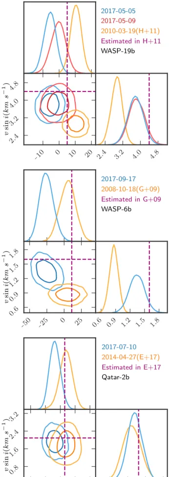
−60 −40 −20 0 ₂₀ λ(◦) 4.5 6.0 7.5 9.0 v sin i( k m s − 1 ) 4.5 6.0 7.5 9.0 v sin i(km s−1) 2017-07-12 2017-07-19 2017-09-04 2007-09-02(B+08) Estimated in B+08 CoRoT-2b −10 0 _{10 20} λ(◦) 2.4 3.2 4.0 4.8 v sin i( k m s − 1 ) 2.4 3.2 4.0 4.8 v sin i(km s−1) 2017-05-05 2017-05-09 2010-03-19(H+11) Estimated in H+11 WASP-19b −15 0 ₁₅ λ(◦) 1.2 1.6 2.0 2.4 v sin i( k m s − 1 ) 1.2 1.6 2.0 2.4 v sin i(km s−1) 2017-04-15 2017-04-21 2011-04-03(N+16) Estimated in N+16 WASP-41b −50 −25 0 ₂₅ λ(◦) 0.6 0.9 1.2 1.5 1.8 v sin i( k m s − 1 ) 0.6 0.9 1.2 1.5 1.8 v sin i(km s−1) 2017-09-17 2008-10-18(G+09) Estimated in G+09 WASP-6b −20 0 20 40 λ(◦) 1.6 2.4 3.2 4.0 v sin i( k m s − 1 ) 1.6 2.4 3.2 4.0 v sin i(km s−1) 2017-09-21 2011-08-21(H+13) Estimated in H+13 WASP-52b −100 −50 0 50 100 λ(◦) 0.8 1.6 2.4 3.2 v sin i( k m s − 1 ) 0.8 1.6 2.4 3.2 v sin i(km s−1) 2017-07-10 2014-04-27(E+17) Estimated in E+17 Qatar-2b

Fig. 1.Posterior probability distributions in v sin i_{−λ parameter space of all our targets obtained from the fit to individual} RM observations obtained at different transits and on different nights. Each panel shows different planetary system, and in each panel different colors correspond to the different nights on which the RM observation were performed. The purple 3

Table 1.Planetary and stellar parameters of our targets

Parameter Symbol Unit WASP-6b WASP-19b WASP-41b WASP-52b CoRoT-2b Qatar-2b

Stellar radius R? R 0.87 1.004 1.01 0.79 0.902 0.713

Planet-to-star radius ratio Rp/R? - 0.1463 0.1488 0.13674 0.16462 0.1667 0.16208

Scaled semimajor axis a/R? - 10.4085 3.552 9.96 7.38 6.70 5.98

Orbital inclination i ◦ 88.47 78.94 88.7 85.35 87.84 86.12

Orbital period P days 3.3610060 0.78884 3.0524040 1.7497798 1.7429935 1.33711647

Linear limb darkening u1 - 0.386 0.427 0.3 0.62 0.346 0.6231

Quadratic limb darkening u2 - 0.214 0.222 0.25 0.06 0.220 0.062

Table 2.Summary of RM observation nights, and the simultaneous photometry

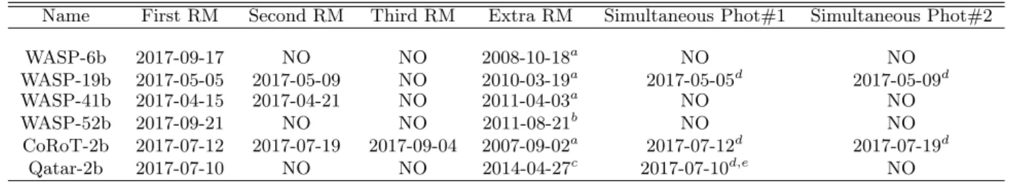
Name First RM Second RM Third RM Extra RM Simultaneous Phot#1 Simultaneous Phot#2

WASP-6b 2017-09-17 NO NO 2008-10-18a NO NO WASP-19b 2017-05-05 2017-05-09 NO 2010-03-19a 2017-05-05d 2017-05-09d WASP-41b 2017-04-15 2017-04-21 NO 2011-04-03a NO NO WASP-52b 2017-09-21 NO NO 2011-08-21b NO NO CoRoT-2b 2017-07-12 2017-07-19 2017-09-04 2007-09-02a 2017-07-12d 2017-07-19d Qatar-2b 2017-07-10 NO NO 2014-04-27c 2017-07-10d,e NO a _HARPS b_SOPHIE c _HARPS-N d_TRAPPIST e _SPECULOOS

We list all the planetary and stellar parameters of our targets collected from the literature and that are necessary for our analysis in Table 1.

2.2. HARPS observation

Our program was allocated 60 hours on the HARPS spec-trograph, mounted on the ESO 3.6 m telescope at La Silla observatory (Mayor et al. 2003), to carry out high-precision RV measurements during three transits of each of our targets (under ESO programme ID: 099.C-0093, PI: M. Oshagh). The main aim of our program was to measure the spin-orbit angle λ from individual RM observation of each target, by having multiple λ measurements for each target, and to quantify the changes in the measured λ from transit to transit.

Thanks to the time-sharing scheme on HARPS with sev-eral other observing programs we were able to spread our 60 hours (equivalent to six nights) over a large fraction of the semester and obtain observations during several nights in which transits occur. Due to bad weather we lost almost 35% of our allocated time, thus we could not obtain three RM observations for all of our targets. We summarize the number of RM observations collected for each target and the nights in Table 2. To overcome the shortage of several RM observations for some of our targets, we decided to collect the publicly available RM observations, preferably obtained with HARPS, of those targets (called extra RM). The extra RM observations, their observed dates, and the spectrograph are also listed in Table 2.

The RM observation for each transit started at least one hour before the start of the transit and lasted until one hour after the transit ended. The exposure times range from 900 to 1200 seconds, ensuring a constant signal-to-noise ra-tio. All our targets throughout the observations remained

above airmass 1.8 (X < 1.8). The spectra were acquired with simultaneous Fabry–Perot spectra on fiber B for si-multaneous wavelength reference, and were taken with the detector in fast-readout mode to minimize overheads and increase the total integration time during transit.

The collected HARPS spectra in our study were reduced using the HARPS Data Reduction Software (DRS - Pepe et al. 2002; Lovis & Pepe 2007). The spectra were cross-correlated with masks based on their stellar spectral type. As output the DRS provides the RVs and associated error.

2.3. TRAPPIST/SPECULOOS observations

We obtained additional simultaneous high-precision pho-tometric transit observations with some of our RM ob-servations using TRAPPIST-South3 _{(Gillon et al. 2011;} Jehin et al. 2011), and one of the SPECULOOS4 _Southern Observatory telescopes (Gillon 2018; Burdanov et al. 2017). TRAPPIST-South is a 60 cm (F/8) Ritchey–Chr´etien tele-scope installed by the University of Li`ege in 2010 at the ESO La Silla Observatory in the Atacama Desert in Chile. The SPECULOOS Southern Observatory is a fa-cility composed of four robotic Ritchey–Chr´etien (F/8) telescopes of 1 m diameter currently being installed at the ESO Paranal Observatory (PI of both telescopes: M. Gillon). The main objective of obtaining simultaneous high-precision and high-cadence photometric transit light curves was to assist us in identifying the presence of occultations of active regions by the planet during the transits. We listed the nights on which simultaneous photometric transits were collected in Table 2.

The observation for each transit started at least one hour before the start of the transit and lasted until one hour

3 _{www.trappist.uliege.be} 4 _{www.speculoos.uliege.be}

after the transit ended. The TRAPPSIT and SPECULOOS observations were acquired in V band and Sloan g’, respec-tively. The exposure times range from 10 to 35 seconds.

Data reduction consisted of standard calibration steps (bias, dark, and flat-field corrections) and subsequent aper-ture photometry in IRAF/DAOPHOT Stetson (1987). Comparison stars and aperture size were selected manually to ensure the best photometric quality in terms of the flux standard deviation of check stars, i.e., non-variable stars similar in terms of magnitude and color to the target star.

3. Variation of spin-orbit angle

In this section we aim to determine the changes in measured spin-orbit angle λ estimated from individual RM observa-tions for a sample of exoplanets.

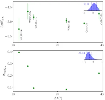
13 28 43 −5.5 −5.0 −4.5 log R 0 HK CoRoT-2b Qatar-2b W ASP-6b W ASP-19b W ASP-41b W ASP-52b 0.11 −1 0 1 13 28 43 ∆λ(◦₎ 0.1 0.2 0.3 0.4 σlog R 0 HK -0.44 −1 0 1

Fig. 2.Top: Correlations between ∆λ and logR0HK. At the top right the calculated value of ρ and also its posterior dis-tribution is presented. The dashed vertical lines indicate the 68% highest posterior density credible intervals (Figueira et al. 2016). Bottom: Same as top but for ∆λ and σlogR0

HK.

3.1. RM model

To estimate the spin-orbit angle λ from RM observations, we use the publicly available code ARoME5 _{(Bou´e et al.} 2012), which provides an analytical model to compute the RM signal, and is optimized for the spectrographs that utilize the CCF-based approach to estimate RVs (such as HARPS). ARoME requires as input parameters the width of a non-rotating star which can be considered as the instru-mental broadening profile (β0), width of the best Gaussian fit to out-of-transit CCF (σ0), stellar macroturbulence (ζ), stellar radius (R?), projected stellar rotational velocity v sin i, stellar quadratic limb darkening coefficients (u1and u2), planetary semimajor axis (a), orbital period of planet (P ), planet-to-star radius ratio (Rp/R?), orbital inclination

5 _{www.astro.up.pt/resources/arome}

angle (i), and the spin-orbit angle λ in order to calculate the RM signal.

Brown et al. (2017) performed a comparison study be-tween ARoME and other RM modeling tools, and reached the conclusion that ARoME consistently underestimates v sin i when compared to other models. Although v sin i dif-fered, the estimated λ were in strong agreement for all the models. Moreover, ARoME is the only code which is pub-licly available, and we are only interested in estimating λ and in its variation, thus we decided to use the ARoME tool for our analysis.

3.2. Fitting RM observation

As the first step of our analysis we carry out a least-squares linear fit to the out-of-transit RV data of each observed RM observations for each planet, and remove the linear trend. The main purpose of this is to eliminate the RV contribution from the Keplerian orbit (which we assume to be linear for the period of observations)6_{, the systematics,} and also the stellar activity which induces RV slopes to the out-of-transit RV data points (Boldt et al. in prep. 2018). After the linear trend is removed, we fit individual RM observation with the ARoME model.

In our fitting procedure we consider the spin-orbit an-gle (λ) , projected stellar rotational velocity (v sin i), and the mid-transit time (T0) as our free parameters. Due to presence of degeneracy between λ and v sin i, especially for a low-impact parameter system (Brown et al. 2017), fre-quently these are the two common free parameters in fit-ting and analyzing RM signals. Since ARoME generates an RM signal centered around zero time (assuming zero as the mid-transit), we have to remove the mid-transit times (cal-culated based on the reported ephemeris and orbital period of the planet) from our observation 7_{. Due to the} uncer-tainty on the reported value of the ephemeris and also the possible variation in transit time (due to the presence of an unknown companion in the systems) the calculated T0 might not be very accurate; thus, we decided to leave T0 as the third free parameter. It could be argued that the slope of the out-of-transit trend should be one of our free parameters in the fitting RM, but since Boldt et al. (in prep. 2018) demonstrated that trend removal does have a negligible impact on the spin-orbit angle λ estimation, we decided to fit the slope and remove the trend prior to our RM fitting procedure. Nonetheless, to evaluate our choice, we explore the consequences of leaving the slope as an extra free parameter in our fitting procedure in Appendix A. The result of that test indicates that the impact is negligible on the other parameters, which support our choice.

The rest of the parameters required in ARoME, such as stellar radius (R?), quadratic limb darkening coefficients of the star (u1 and u2), the semimajor axis of the planet, the orbital period of planet(a), and the planetary orbital inclination angle (i), are fixed to their reported values in the literature (which are given in Table 1). We also fixed the macro-turbulence velocity of all stars to ζ = 4kms−1

6 _{Using the shortest period of our sample, 0.78 days, the}

transit duration of 1.9 hours corresponds to 10 % of the to-tal phase, which supports our assumption of a linear trend from the Keplerian orbit.

7

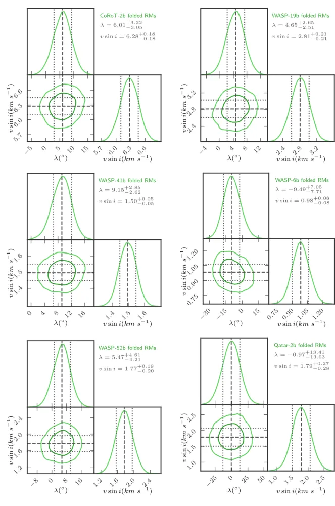
−5 0 5 10 15 λ(◦) 5.7 6.0 6.3 6.6 v sin i( k m s − 1 ) 5.7 6.0 6.3 6.6 v sin i(km s−1) CoRoT-2b folded RMs λ = 6.01+3.22_−3.05 v sin i = 6.28+0.18_−0.18 −4 0 4 8 12 λ(◦) 2.4 2.8 3.2 v sin i( k m s − 1) 2.4 2.8 3.2 v sin i(km s−1) WASP-19b folded RMs λ = 4.65+2.65_−2.51 v sin i = 2.81+0.21_−0.21 0 4 8 _{12 16} λ(◦) 1.4 1.5 1.6 v sin i( k m s − 1 ) 1.4 1.5 1.6 v sin i(km s−1) WASP-41b folded RMs λ = 9.15+2.85_−2.62 v sin i = 1.50+0.05_−0.05 −30 −15 0 15 λ(◦) 0.75 0.90 1.05 1.20 v sin i( k m s − 1 ) 0.75 0.90 1.05 1.20 v sin i(km s−1) WASP-6b folded RMs λ =−9.49+7.05_−7.71 v sin i = 0.98+0.08_−0.08 −8 0 8 16 λ(◦) 1.2 1.6 2.0 2.4 v sin i( k m s − 1 ) 1.2 1.6 2.0 2.4 v sin i(km s−1) WASP-52b folded RMs λ = 5.47+4.61_−4.21 v sin i = 1.77+0.19_−0.20 −25 0 25 50 λ(◦) 1.0 1.5 2.0 2.5 v sin i( k m s − 1) 1.0 1.5 2.0 2.5 v sin i(km s−1) Qatar-2b folded RMs λ =−0.97+13.41_−13.03 v sin i = 1.79+0.27_−0.28

Fig. 3. Posterior probability distributions in v sin i_{− λ parameter space of all our targets obtained from the fit to the} folded RM observations. Each panel shows different planetary system. The black dashed line displays median values of the posterior distributions, and the 1σ uncertainties taken to be the value enclosed in the 68.3 percent of the posterior distributions are shown with the black dotted line.

−200 −100 0 100 200 300 R V (m/s)

Best fit CoRoT-2b 2017-07-12 RM 2017-07-19 RM 2017-09-4 RM 2007-09-02 RM

−0.06 −0.04 −0.02 0.00 0.02 0.04 0.06 Time midtransit (days)

−100 0 100 Residual −75 −50 −25 0 25 50 75 R V (m/s)

Best fit WASP-19b 2017-05-05 RM 2008-05-09 RM 2010-03-19 RM

−0.06 −0.04 −0.02 0.00 0.02 0.04 0.06 Time midtransit (days)

−50 0 50 Residual −30 −10 10 30 50 R V (m/s)

Best fit WASP-41b 2017-04-15 RM 2008-04-21 RM 2011-04-03 RM

−0.06 −0.04 −0.02 0.00 0.02 0.04 0.06 Time midtransit (days)

0 20 Residual −30 −10 10 30 50 R V (m/s)

Best fit WASP-6b 2017-09-17 RM 2008-10-18 RM

−0.06 −0.04 −0.02 0.00 0.02 0.04 0.06 Time midtransit (days)

−25 0 25 Residual −60 −30 0 30 60 R V (m/s)

Best fit WASP-52b 2017-09-21 RM 2011-08-21 RM

−0.06 −0.04 −0.02 0.00 0.02 0.04 0.06 Time midtransit (days)

−50 0 50 Residual −60 −20 20 60 100 R V (m/s)

Best fit Qatar-2b 2017-07-10 RM 2014-04-27 RM

−0.06 −0.04 −0.02 0.00 0.02 0.04 0.06 Time midtransit (days)

−50 0 50

Residual

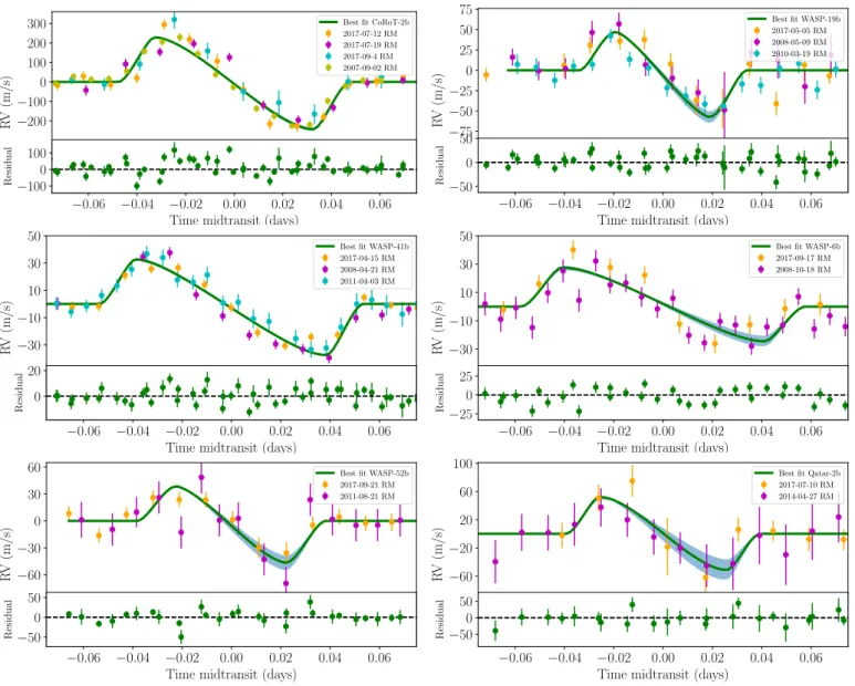
Fig. 4.Folded RM observations of our targets during several nights. The green line shows the best fitted RM model and blue region shows the zone where 68% of the model solutions reside. In each panel the residuals are shown in the bottom panel.

Table 3.Details of the priors that we apply during our MCMC analysis

Parameter WASP-6b WASP-19b WASP-41b WASP-52b CoRoT-2b Qatar-2b

λ(◦_{) U(−180; +180) U(−180; +180) U(−180; +180) U(−180; +180) U(−180; +180) U(−180; +180)} v sin i(kms−1_{)N (1.6; 0.6) N (5.1; 0.5) N (2.66; 0.5) N (3.6; 0.5) N (11.25; 4.) N (2.09; 0.5)} T0(JD) N (8014.57580; 0.01) N (7878.63066; 0.01) N (7858.64562; 0.01) N (8017.65153; 0.01) N (7946.62577; 0.01) N (7945.50129; 0.01) Notes:U(a; b) is a uniform prior with lower and upper limits of a and b; N (µ; σ) is a normal distribution with mean µ and width σ. T0 mean reported is the first transit time for each planet.

and fixed the instrumental broadening according to the HARPS instrument profile (β0 = 1.3kms−1). We would like to note that the macro-turbulence might not be an accurate estimate, but since we are only interested in the variation in λ, the inaccurate macro-turbulence will be the same on all our measured λ. We also evaluate having macro-turbulence as an extra free parameter in our fitting proce-dure in Appendix B. Its results also demonstrate that the impact is negligible on the other parameters, which

sup-ports our choice.We also fixed the width of the Gaussian (σ0) to the width of a Gaussian fit to the CCF of out-of-transit for each star. We note that we have two strong arguments for not letting these parameters be free in our fitting procedure. The first is that we want to have very similar fitting procedures to most of the RM studies, which only use λ and v sin i as free parameters and fix the rest of the parameters to the values obtained from photometric transit. The second reason is based on the small number of

Table 4.Best fitted values for λ and v sin i obtained from each RM observations.

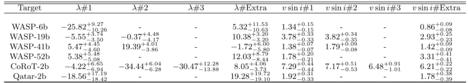
Target λ#1 λ#2 λ#3 λ#Extra v sin i#1 v sin i#2 v sin i#3 v sin i#Extra WASP-6b −25.82+9.27 −10.26 - - 5.32+11.53−10.63 1.34+0.15−0.15 - - 0.86+0.09−0.08 WASP-19b −5.55+3.74 −3.50 −0.37+4.48−4.17 - 10.38+3.20−3.20 3.78+0.33−0.33 3.82+0.34−0.35 - 2.93+0.25−0.23 WASP-41b 5.47+4.45_−4.60 19.39+4.01_−3.86 - −1.72_−5.80+6.00 1.38+0.07_−0.07 1.79+0.09_−0.08 - 1.42+0.09_−0.09 WASP-52b 5.38+5.48_−5.08 - - 12.03_−8.44+8.79 1.78+0.20_−0.21 - - 3.31+0.41_−0.41 CoRoT-2b −4.22+6.65 −6.94 −34.44+6.04−6.28 −30.47+12.28−13.88 8.05+4.06−3.73 7.29+0.44−0.44 7.17+0.51−0.53 6.48+0.91−1.01 6.21+0.22−0.22 Qatar-2b −18.56+17.19_−18.42 - - 19.28_−19.10+19.72 1.92+0.31_−0.33 - - 1.78+0.38_−0.39 Notes:a Obtained from recurring starspot occultations in photometric transit observations,b (Tregloan-Reed et al. 2015),c (Tregloan-Reed et al. 2013),d(Southworth et al. 2016),e (Mancini et al. 2017),f (Nutzman et al. 2011),g (Moˇcnik et al. 2017)

Table 5.Best fitted values for λ and v sin i obtained from folded RM observations.

Parameter WASP-6b WASP-19b WASP-41b WASP-52b CoRoT-2b Qatar-2b λ(◦) −9.49+7.05

−7.71 4.65+2.65−2.51 9.15+2.85−2.65 5.47+4.61−4.21 6.01+3.22−3.05 0.97+13.41−13.03

v sin i(kms−1) 0.98+0.08_−0.08 2.81+0.21_−0.21 1.50+0.05_−0.05 1.77+0.19_−0.20 6.28+0.18_−0.18 1.79+0.27_−0.28 Starspot crossing λ(◦)a 7.2 ± 3.7b 1.0 ± 1.2c 6 ± 11d 3.8 ± 8.4e 4.7 ± 12.3f 0 ± 8g

Notes:a Obtained from recurring starspot occultations in photomteric transit observations,b(Tregloan-Reed et al. 2015),c (Tregloan-Reed et al. 2013),d(Southworth et al. 2016),e (Mancini et al. 2017),f (Nutzman et al. 2011),g (Moˇcnik et al. 2017)

data points in each RM observation. Thus, if we consider all these parameters free we would have more free parameters than observations and we might end up with an overfitted model.

The best fit parameters and associated uncertainties in our fitting procedure are derived using a Markov chain Monte Carlo (MCMC) analysis, using the affine invariant ensemble sampler emcee (Foreman-Mackey et al. 2013). The prior on v sin i and T0are controlled by Gaussian priors centered on the reported value in the literature and width according to the reported uncertainties, and the prior on λ is also controlled by a uniform (uninformative) prior be-tween±180◦_{. We list the selected type of priors and ranges} for our free parameters for each target in Table 3.

We randomly initiated the initial values for our free pa-rameters for 30 MCMC chains inside the prior distribu-tions. For each chain we used a burn-in phase of 500 steps, judging the chain to be converged, and then again sampled the chains for 5000 steps. Thus, the results concatenated to produce 150000 steps. We determined the best fitted values by calculating the median values of the posterior distribu-tions for each parameters, based on the fact that the poste-rior distributions were Gaussian. The 1σ uncertainties were taken to be the value enclosed in the 68.3 % of the posterior distributions.

3.3. Significant variation of spin-orbit angle

Figure 1 shows the posterior distributions in v sin i_{− λ} pa-rameter space of all our targets delivered by the fit to in-dividual RM obtained during different transits on different nights. We listed the best fitted values of λ and v sin i from individual RM observations in Table 4. We found that the estimated spin-orbit angle λ of an exoplanet can be sig-nificantly altered (up to 42◦_{) from transit to transit due} to variation in the configurations of the stellar active re-gions on different nights (mainly as a consequence of the stellar rotation and also the evolution of the stellar active

regions)8_{. The estimated λ variation was larger than the} simulation’s result we described in a previous work, which suggested a variation of up to 15◦_{for hot Jupiters (Oshagh} et al. 2016). The uncertainty on the estimated λ also varies significantly from transit to transit.

The estimated v sin i from the ARoME fit, as mentioned in Brown et al. (2017), are usually underestimated in com-parison to their literature values; however, our goal here is not to measure their value accurately but to evaluate their variation from transit to transit. Our results depict a devi-ation of estimated v sin i from transit to transit; however, for most of the cases the variations are in the uncertainty ranges, and thus could be considered insignificant. However, we would like to note again that since ARoME generally underestimates v sin i this result should be taken with a grain of salt.

The fitted transit time T0for all of our targets coincided with the respective calculated value (based on assuming an unperturbed Keplerian orbit with fixed periodic planetary orbit and according to reported ephemeris). Therefore, we conclude that our observations do not exhibit any signs of transit time variation for any of our targets. However, we would like to note that there might still be transit timing variation in our targets, but we could not detect it due to the small number of points in our RM observations, which prevented us from achieving high-precision transit time es-timations.

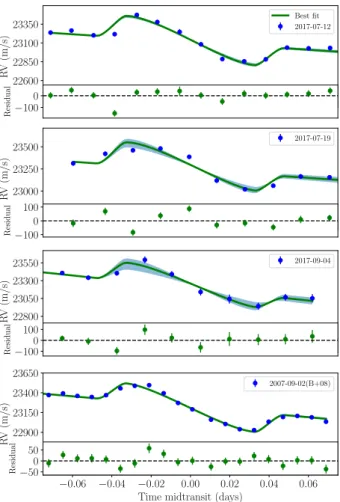
We present each individual RM observation (obtained during different nights) for each of our targets with their best fitted model in Figures C.1–C.6 (Appendix C).

8 _{There could be reasons other than stellar activity that}

4. Probing the correlations between

logR

and

spin-orbit angle variation

In this section we assess the presence of any meaningful cor-relation between the amplitude of the variation of spin-orbit angle (largest variation ∆λ) and measured stellar activity indicator logR0

HK9 . The values of logR0HKs were deliv-ered as a by-product of DRS (as described in Lovis et al. 2011). We calculated the mean of measured logR0

HKs for our stars during our observation, and used the mean value as the measured logR0HK. We also measured the standard deviation of logR0

HKs and used it as the uncertainty on the measured σlogR0

HK. The value of σlogR0HK by itself can also provide information about the variation in magnetic activ-ity of stars during our observation, due to a stellar active region either appearing or disappearing or to the occulta-tion of the active region by a transiting planet.

We inspected the presence of a correlation based on the Spearman’s rank-order correlation coefficient (ρ)10_{. We} evaluated the significance of correlation using the Bayesian approach described in Figueira et al. (2016). The poste-rior distribution of ρ indicates the range of ρ values that is compatible with the observations.

Figure 2, top panel, presents the correlations between ∆λ and logR0

HK. We note that Qatar-2, due to its faint-ness (V = 13.3) and low signal-to-noise ratio in the region of spectrum in which logR0

HKis estimated, has only one es-timated logR0HK; therefore, it was impossible to measure its σlogR0

HK. As this figure shows, there is no meaningful cor-relation between the measured value of ∆λ and logR0

HK. Figure 2, bottom panel, displays the correlations between ∆λ and σlogR0

HK, which show an anti-correlation but not a significant correlation. We note that in this plot we dis-carded Qatar-2.

5. Folding several RM observations

The most logical approach for eliminating the effect of stel-lar activity on RM observations, and thus minimizing its impact on the estimated spin-orbit angle λ, is to obtain several RM observations and combine and fold them. This is based on the fact that the configuration of the stellar active region evolves from transit to transit, but the plan-etary RM signal remains constant; thus, averaging several RM observations will average out the activity noise and in-crease the planetary RM signal-to-noise ratio. Therefore, in this section we fold all the observed RM observations for each planet (analyzed in the previous section), and try to repeat the fitting procedure to estimate more accurately the spin-orbit angle λ and the host star v sin i .

In order to fold all the available RM observations for each target, we utilize the best fitted transit time (T0) ob-tained in the previous section. Therefore, in our fitting pro-cedure we no longer leave the transit time as a free param-eter, thus λ and v sin i are our only free parameters.

Figure 3 presents the posterior distributions from the fit to folded RM observations of all of our targets, and displays

9 _logR0

HK is one of the most powerful chromospheric activity

indicators and is estimated by measuring the excess flux in the core of Ca ii H+K lines, normalized to the bolometric flux.

10 _{Spearman’s rank-order correlation assesses how well two}

variables can be described with a monotonic relationship that is not purely linear.

the best fitted values for λ and v sin i and their associated 1σ uncertainties. We summarized the best fitted values in Table 5. Moreover, in Table 5 we also list the estimated values of λ for our targets, which were estimated from an independent method of recurring starspot occultations in photometric transit light curve observations. The compari-son between our estimated λ from folded RM observations and those measured from recurring starspot occultations (both presented in Table 5) reinforce that the strategy of folding RM observations adequately eliminates the stellar activity effect, and provides an accurate estimate of λ. We present the folded RM observations for each of our targets and their best fitted model in Figure 4.

6. Simultaneous photometric transit light curve

and RM observations

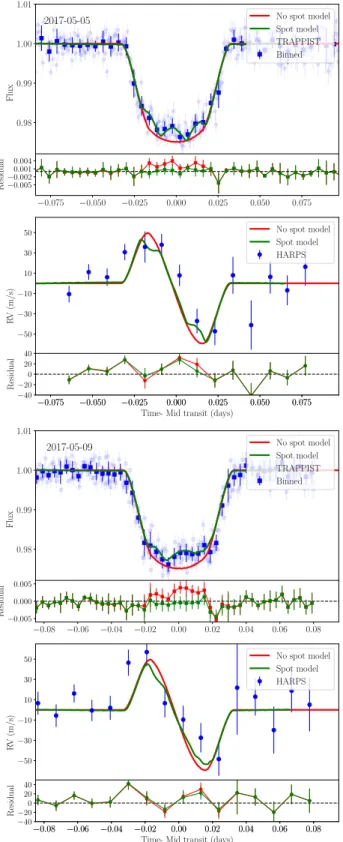
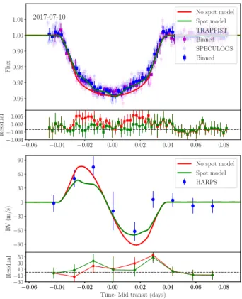
Photometric transit observations can usually be acquired on much shorter exposure times than RM observations11_, and thus could lead to the easier and clearer detection of the occultation of active regions during the transit of an ex-oplanet. We obtained five simultaneous photometric tran-sit observations with our RM observations, four with the TRAPPSIT telescope and one with SPECULOOS. All the photometric transit light curves clearly indicated the pres-ence of active regions’ crossing. Thus, the main aim of this section is to assess whether we can have a better RM mod-eling by having the information from the active region’s crossing event during a photometric transit (which provides information about the size, position, and contrast of active regions).

6.1. Fitting photometric transit anomalies with SOAP3.0 In this section we use the publicly available tool SOAP3.0. This tool has the capability of simulating a transiting planet and a rotating star covered with active regions, and delivers photometric and RV variation signals. SOAP3.0 takes into account not only the flux contrast effect in these regions, but also the RV shift due to inhibition of the convective blueshift inside these regions. SOAP3.0 also takes into ac-count the occultation between the transiting planet and active regions in its calculation of transit light curve and RM.

We use SOAP3.0 to obtain the best fitted model to the photometric transit light curves and then compare the cor-responding RM of the best fitted model with the observed RM observations. Because of the slowness of SOAP3.0, due to its numerical nature in comparison to the analytical nature of ARoMe, performing an MCMC approach using SOAP3.0 is not feasible. Therefore, we decided to perform a χ2

reducedminimization using SOAP3.0 to fit the active re-gion crossing events in the photometric transit light curves. From visual inspection we could identify only three active region crossing events during each observed transit light curve, thus we decided to fix the number of active regions to three. In χ2

reducedminimization we fixed all the required

11

Spectrographs lose photons due to slit losses, stray light, and scattered light. Moreover, spectrographs disperse photons over the detector where each pixel has a different readout noise. Therefore, spectrograph by construction required many more photons to reach the same S/N as photometric observations.

Table 6.Standard deviation of the residual between SOAP3.0 predicted RM and observed RM for models that ignore the spot crossing events and for models that take into account spot crossing events.

Standard deviation (ms−1) CoRoT-2b#1 CoRoT-2b#2 WASP-19b#1 WASP-19b#2 Qatar-2b

No spot 33.862 82.58 18.75 18.22 23.09

With spot 27.93 65.77 16.50 17.23 18.56

parameters of stars and planets in SOAP3.0 (the same pa-rameters in Table 1) except for the three active regions’ parameters (filling factor, location, and temperature con-trast) and let them vary as free parameters. The range of free parameters which were explored are listed as the spots’ filling factor [0.1%:20%], latitude [−90◦_:+90◦_], lon-gitude [0◦_:360◦_{], and temperature contrast [0:−T}

ef f].

6.2. Improved RM prediction

As mentioned before, here we intend to compare the corre-sponding RM of the best fitted model to the transit light curves with the observed RM 12_{. We overplotted the RM} counterpart of the best fitted model over the simultaneous observed RM observations for WASP-19b, CoRoT-2b, and Qatar-2b in Figures 5, 6, and 7, respectively. This result demonstrated that the RM counterparts coincide much bet-ter with the observed RM. As a consequence, the residual between the SOAP3.0 RM whose considered active region crossing is lower than the residual of SOAP3.0 RM without any spot crossing event. To quantify the improvement, we computed the standard deviation of the residual between SOAP3.0 best fit predicted RM and the observed RM, for models ignoring stellar spots and for models taking them into account. All standard deviations are listed in Table 6, and they all support the improvement in the RM predic-tion.

It is worth mentioning that a strong degeneracy exists between the parameters of the stellar active regions; for in-stance, different filling factor, position, and contrast could produce very similar photometric signatures while gener-ating completely different RV signals. Therefore, we have to clarify our best fitted model to the photometric transit light curves, and also the best fitted value for the active regions’ parameters might not correspond to accurate val-ues, although they more closely predict the RM observation than considering no active region occultation.

7. Discussion

Estimation of λ and v sin i could be influenced by second-order effects such as the stellar convective blueshift and granulation (Shporer & Brown 2011; Cegla et al. 2016b), the microlensing effect due to the transiting planet’s mass Oshagh et al. (2013a), the impact of ringed exoplanet on RM signal (Ohta et al. 2009; de Mooij et al. 2017; Akinsanmi et al. 2018), and stellar differential rotation (Albrecht et al. 2012; Cegla et al. 2016a; Serrano et al. in prep. 2018). However, their expected signals in RM obser-vations are different from the active region crossing events. More importantly, all of their signals are constant during

12 _{We did not perform SOAP3.0 fitting to the RM observation,}

and we only fitted SOAP3.0 to the photometric transit-light curve and used the corresponding RM of the best fitted model.

several transits; thus, even if they affect the estimation of λ and v sin i, their influence cannot produce variation in the estimated λ. Therefore, of the extensive list of effects above, we can conclude that the variation in the estimated λ could have only originated from the stellar activity noise. The simulations presented in Oshagh et al. (2016) pre-dicted that the variation in estimated λ could reach up to 15◦ _{for hot Jupiters; however, our observational campaign} shows a variation that is twice as large. The plausible ex-planation for this underestimation of variation in the sim-ulation could be that in the simsim-ulation the stellar active regions were considered to be similar to the sunspots (e.g., a filling factor of around 1%). However, all the stars in our sample exhibit a much higher level of activity than the Sun, and are covered with much larger stellar spots (fill-ing of stellar spots on the WASP-6, WASP-19, WASP-41, WASP-52, CoRoT-2, and Qatar-2 were 6%, 8% , 3%, 15%, 16%, and 4%, respectively).

We would like to note that throughout one RM ob-servation the target’s airmass varies, and also from one night to another the mid-transit occurs at different airmass. Moreover, the seeing condition fluctuates from night to night. Therefore, there could be some considerable contri-bution from airmass and seeing variations which might lead to the variation in observed RM observations. Although this statement is provable, correcting their effect is not a trivial task and beyond the scope of the current study. However, this again points to the fact that having only single-epoch RM observation could be vulnerable to other unaccounted noise sources. Moreover, we would like to suggest obtaining several RM observations of a planet transiting a very inac-tive star to be able to better explore the seeing and airmass conditions on the estimated λ.

We showed that folding several RM observation could mitigate the impact of stellar active region occultation; however, if RM observation are done on consecutive tran-sits, and are not separated with long time interval from each other, we would like to note that they can be affected by oc-cultation with the same active regions, and thus folding the RM observations will not improve the accuracy of the es-timation of λ. Therefore, we suggest obtaining several RM observations with a long time separation compatible with several stellar rotations to ensure that RM observations are affected by the configurations of different active regions.

Our results also highlighted the power of having simul-taneous photometric transit observations with RM observa-tions, which provides unique information about the stellar active regions that have been occulted during the transit, and leads to a better elimination of their influence on the observed RM. Thus, in the cases where only one RM obser-vation can be observed (e.g., due to the long periodicity of the planet) and the combination of several RM observations is not feasible, having simultaneous photometric transit will be needed and crucial. Although, one missing piece in

an-0.96 0.97 0.98 0.99 1.00 1.01 Flux

2017-07-12 No spot model_{Spot model} TRAPPIST Binned −0.075 −0.050 −0.025 0.000 0.025 0.050 0.075 0.100 −0.006 −0.003 0.000 0.003 0.006 Residual −0.075 −0.050 −0.025 0.000 0.025 0.050 0.075 0.100 −300 −200 −100 0 100 200 300 R V (m/s) No spot model Spot model HARPS −0.075 −0.050 −0.025 0.000 0.025 0.050 0.075 0.100 Time- Mid transit (days)

−60 −30 0 30 Residual 0.96 0.97 0.98 0.99 1.00 1.01 Flux

2017-07-19 No spot model_{Spot model} TRAPPIST Binned −0.075 −0.050 −0.025 0.000 0.025 0.050 0.075 0.100 −0.008 −0.003 0.002 0.007 0.012 Residual −0.075 −0.050 −0.025 0.000 0.025 0.050 0.075 0.100 −300 −200 −100 0 100 200 300 R V (m/s) No spot model Spot model HARPS −0.075 −0.050 −0.025 0.000 0.025 0.050 0.075 0.100 Time- Mid transit (days)

−120−70 −2030 80 130

Residual

Fig. 5. Simultaneous photometric transit and RM obser-vation of CoRoT-2b on the night of 2017-07-12 (top pan-els) and on night the night of 2017-07-19 (bottom panpan-els). The dark blue square represents the binned TRAPPIST photometric observations, and the dark blue filled circle the HARPS RM observation. The red line is the SOAP3.0 model without considering any stellar active regions. The green lines are the SOAP3.0 best fitted model to transit light curve taking into account three spots.

0.98 0.99 1.00 1.01 Flux 2017-05-05 No spot model Spot model TRAPPIST Binned −0.075 −0.050 −0.025 0.000 0.025 0.050 0.075 −0.005 −0.0020.001 0.004 Residual −0.075 −0.050 −0.025 0.000 0.025 0.050 0.075 −50 −30 −10 10 30 50 R V (m/s) No spot model Spot model HARPS −0.075 −0.050 −0.025 0.000 0.025 0.050 0.075 Time- Mid transit (days)

−40 −20 0 20 40 Residual 0.98 0.99 1.00 1.01 Flux 2017-05-09 No spot model Spot model TRAPPIST Binned −0.08 −0.06 −0.04 −0.02 0.00 0.02 0.04 0.06 0.08 −0.005 0.000 0.005 Residual −0.08 −0.06 −0.04 −0.02 0.00 0.02 0.04 0.06 0.08 −50 −30 −10 10 30 50 R V (m/s) No spot model Spot model HARPS −0.08 −0.06 −0.04 −0.02 0.00 0.02 0.04 0.06 0.08 Time- Mid transit (days)

−40 −20 0 20 40 Residual

Fig. 6. Simultaneous photometric transits and RM obser-vations of WASP-19b on the night of 2017-05-05 (top pan-els) and on the night of 2017-05-09 (bottom panpan-els). The lines and points are the same as in Fig. 3.

alyzing simultaneous photometric and RM observations is the lack of an analytical model, similar to ARoME which takes into account the active region occulation in RM mod-eling, which reduces significantly the computational cost and allows a more robust fitting utilizing the MCMC ap-proach.

0.96 0.97 0.98 0.99 1.00 1.01 Flux

2017-07-10 No spot model_{Spot model} TRAPPIST Binned SPECULOOS Binned −0.06 −0.04 −0.02 0.00 0.02 0.04 0.06 0.08 −0.004 −0.001 0.002 0.005 Residual −0.06 −0.04 −0.02 0.00 0.02 0.04 0.06 0.08 −90 −60 −30 0 30 60 90 R V (m/s) No spot model Spot model HARPS −0.06 −0.04 −0.02 0.00 0.02 0.04 0.06 0.08 Time- Mid transit (days)

−30 −10 10 30 50 Residual

Fig. 7. Simultaneous photometric transits and RM obser-vations of Qatar-2b on the night of 2017-07-10. The pho-tometric observations were obtained from simultaneous ob-servations of TRAPPIST and SPECULOOS. The lines and points are the same as in Fig. 3.

Complementary methods such as Doppler tomography have been used to estimate the spin-orbit angle λ of a planet around hot and rapidly rotating host stars which the con-ventional RM technique is unable to deal with. However, the impact of a stellar active region (either occulted and unocculted ones) on the Doppler tomography signal has not been explored, and by having our observation data set we will be able to explore this matter. However, probing this effect is beyond scope of the current paper and will be pursued in a forthcoming publication.

Oshagh et al. (2016) predicted that the impact of ac-tive regions’ occultation on the estimated λ will be more significant for the Neptune- or Earth-sized planets. Since the planets in our sample are all hot Jupiters (gas giant exoplanets orbiting very close to their host stars), we can extrapolate and speculate that accurately estimating the spin-orbit angle for a small-sized planet will be a challeng-ing task. As an example of this difficulty and complication for small-sized planet we can point to the case of 55 Cnc e whose different RM observations lead to different interpre-tations regarding its spin-orbit angles (Bourrier & H´ebrard 2014; L´opez-Morales et al. 2014).

If the variations in λ are mostly ascribed to the stel-lar activity, they should depend on the wavelength region where RVs are measured. Therefore, performing chromatic RM observations similar to Di Gloria et al. (2015), and measuring λ variation in different wavelengths could pro-vide information about which wavelength range the stellar activity influence is minimum and thus the estimated λ is more accurate. However, exploring this area is beyond the

scope of the current paper and will be pursued in forthcom-ing publication.

8. Conclusion

Rossiter–McLaughlin observations have provided an effi-cient way to estimate spin-orbit angle λ for more than 200 exoplanetary systems which include planets on highly mis-aligned, polar, and even retrograde orbits. So far, however, mostly single-epoch RM observations have been used to es-timate the spin-orbit angle, and therefore there has been no study evaluating the dependence of estimated spin-orbit angle on induced noise in RM observations. One of the most important and dominant sources of time varying noise in RM observations is stellar activity. In this paper we ob-tained several RM observations of known transiting plan-ets which all transit extremely active stars, and by ana-lyzing them individually we were able to quantify, for the first time, the variation in the estimated spin-orbit angle from transit to transit. Our results reveal that the esti-mated spin-orbit angle can be significantly altered (up to ∼ 42◦_{). This finding is almost two times larger than the} ex-pected variation predicted from the simulation. We could not identify any meaningful correlation between the vari-ation of estimated spin-orbit angles and stellar magnetic activity indicators. We also investigated two possible ap-proaches for mitigating the influence of stellar activity on RM observations. The first strategy is based on obtaining several RM observations and folding them to reduce the stellar activity noise. Our results demonstrate that this is a feasible and robust way to overcome this issue. The second approach is based on acquiring simultaneous high-precision short-cadence photometric transit light curve that can pro-vide more information about the properties of the stellar active region, which will allow a better RM modeling.

Acknowledgements. M.O. acknowledges research funding from the Deutsche Forschungsgemeinschft (DFG, German Research Foundation) -OS 508/1-1. We acknowledge the use of the software packages pyGTC (Bocquet & Carter 2016) and emcee (Foreman-Mackey et al. 2013). The research leading to these results has received funding from the European Research Council (ERC) under the FP/2007-2013 ERC grant agreement no. 336480 and from an Actions de Recherche Concert´ee (ARC) grant, financed by the Wallonia-Brussels Federation (PI Gillon). This work was also partially supported by a grant from the Simons Foundation (PI Queloz, grant number 327127), and by the MERAC foundation (PI Triaud). L.D. acknowledges support from the Gruber Foundation Fellowship. M.G. and E.J. are F.R.S.-FNRS Research Associate and Senior Research Associate, respectively. We would like to thank the referee, Teruyuki Hirano, for his constructive comments and insightful suggestions, which added significantly to the clarity of this paper.

References

Addison, B. C., Tinney, C. G., Wright, D. J., et al. 2013, ApJ, 774, L9

Akinsanmi, B., Oshagh, M., Santos, N. C., & Barros, S. C. C. 2018, A&A, 609, A21

Albrecht, S., Winn, J. N., Johnson, J. A., et al. 2012, ApJ, 757, 18 Barros, S. C. C., Bou´e, G., Gibson, N. P., et al. 2013, MNRAS, 430,

3032

Baruteau, C., Crida, A., Paardekooper, S.-J., et al. 2014, Protostars and Planets VI, 667

Batygin, K. 2012, Nature, 491, 418

Bayliss, D. D. R., Winn, J. N., Mardling, R. A., & Sackett, P. D. 2010, ApJ, 722, L224

Bocquet, S. & Carter, F. W. 2016, The Journal of Open Source Software, 1

Boldt, S., Oshagh, M., Dreizler, S., & Reiners, A. in prep. 2018, A&A Bouchy, F., Queloz, D., Deleuil, M., et al. 2008, A&A, 482, L25

Bou´e, G., Oshagh, M., Montalto, M., & Santos, N. C. 2012, MNRAS, 422, L57

Bourrier, V. & H´ebrard, G. 2014, A&A, 569, A65

Brown, D. J. A., Triaud, A. H. M. J., Doyle, A. P., et al. 2017, MNRAS, 464, 810

Burdanov, A., Delrez, L., Gillon, M., et al. 2017, SPECULOOS Exoplanet Search and Its Prototype on TRAPPIST, 130

Cegla, H. M., Lovis, C., Bourrier, V., et al. 2016a, A&A, 588, A127 Cegla, H. M., Oshagh, M., Watson, C. A., et al. 2016b, ApJ, 819, 67 Cosentino, R., Lovis, C., Pepe, F., et al. 2012, in Proc. SPIE, Vol. 8446, Ground-based and Airborne Instrumentation for Astronomy IV, 84461V

Crida, A. & Batygin, K. 2014, A&A, 567, A42

Czesla, S., Huber, K. F., Wolter, U., Schr¨oter, S., & Schmitt, J. H. M. M. 2009, A&A, 505, 1277

Dai, F., Winn, J. N., Yu, L., & Albrecht, S. 2017, AJ, 153, 40 Dawson, R. I. & Johnson, J. A. 2018, ArXiv e-prints

de Mooij, E. J. W., Watson, C. A., & Kenworthy, M. A. 2017, MNRAS, 472, 2713

Di Gloria, E., Snellen, I. A. G., & Albrecht, S. 2015, A&A, 580, A84 Esposito, M., Covino, E., Desidera, S., et al. 2017, A&A, 601, A53 Figueira, P., Faria, J. P., Adibekyan, V. Z., Oshagh, M., & Santos,

N. C. 2016, Origins of Life and Evolution of the Biosphere, 46, 385 Foreman-Mackey, D., Hogg, D. W., Lang, D., & Goodman, J. 2013,

PASP, 125, 306

Gillon, M. 2018, Nature Astronomy, 2, 344

Gillon, M., Anderson, D. R., Triaud, A. H. M. J., et al. 2009, A&A, 501, 785

Gillon, M., Jehin, E., Magain, P., et al. 2011, in European Physical Journal Web of Conferences, Vol. 11, European Physical Journal Web of Conferences, 06002

H´ebrard, G., Bouchy, F., Pont, F., et al. 2008, A&A, 488, 763 H´ebrard, G., Collier Cameron, A., Brown, D. J. A., et al. 2013, A&A,

549, A134

H´ebrard, G., Ehrenreich, D., Bouchy, F., et al. 2011, A&A, 527, L11 Hellier, C., Anderson, D. R., Collier-Cameron, A., et al. 2011, ApJ,

730, L31

Holt, J. R. 1893, Astronomy and Astro-Physics (formerly The Sidereal Messenger), 12, 646

Ioannidis, P., Huber, K. F., & Schmitt, J. H. M. M. 2016, A&A, 585, A72

Jehin, E., Gillon, M., Queloz, D., et al. 2011, The Messenger, 145, 2 L´opez-Morales, M., Triaud, A. H. M. J., Rodler, F., et al. 2014, ApJ,

792, L31

Lovis, C. & Pepe, F. 2007, A&A, 468, 1115

Mancini, L., Southworth, J., Raia, G., et al. 2017, MNRAS, 465, 843 Mayor, M., Pepe, F., Queloz, D., et al. 2003, The Messenger, 114, 20 McLaughlin, D. B. 1924, ApJ, 60, 22

Moˇcnik, T., Southworth, J., & Hellier, C. 2017, MNRAS, 471, 394 Neveu-VanMalle, M., Queloz, D., Anderson, D. R., et al. 2016, A&A,

586, A93

Nutzman, P. A., Fabrycky, D. C., & Fortney, J. J. 2011, ApJ, 740, L10

Ohta, Y., Taruya, A., & Suto, Y. 2009, ApJ, 690, 1

Oshagh, M., Bou´e, G., Figueira, P., Santos, N. C., & Haghighipour, N. 2013a, A&A, 558, A65

Oshagh, M., Dreizler, S., Santos, N. C., Figueira, P., & Reiners, A. 2016, A&A, 593, A25

Oshagh, M., Santos, N. C., Boisse, I., et al. 2015a, in European Physical Journal Web of Conferences, Vol. 101, European Physical Journal Web of Conferences, 05003

Oshagh, M., Santos, N. C., Boisse, I., et al. 2013b, A&A, 556, A19 Oshagh, M., Santos, N. C., Figueira, P., et al. 2015b, A&A, 583, L1 Pepe, F., Mayor, M., Galland, F., et al. 2002, A&A, 388, 632 Pepe, F., Molaro, P., Cristiani, S., et al. 2014, Astronomische

Nachrichten, 335, 8

Pollack, J. B., Hubickyj, O., Bodenheimer, P., et al. 1996, Icarus, 124, 62

Quirrenbach, A., Amado, P. J., Caballero, J. A., et al. 2014, in Proc. SPIE, Vol. 9147, Ground-based and Airborne Instrumentation for Astronomy V, 91471F

Rossiter, R. A. 1924, ApJ, 60, 15

Sanchis-Ojeda, R. & Winn, J. N. 2011, ApJ, 743, 61

Sanchis-Ojeda, R., Winn, J. N., Marcy, G. W., et al. 2013, ApJ, 775, 54

Santerne, A., H´ebrard, G., Deleuil, M., et al. 2014, A&A, 571, A37 Sedaghati, E., Boffin, H. M. J., Csizmadia, S., et al. 2015, A&A, 576,

L11

Serrano, L., Oshagh, M., Santos, N., & Barros, S. in prep. 2018, A&A Shporer, A. & Brown, T. 2011, ApJ, 733, 30

Southworth, J., Tregloan-Reed, J., Andersen, M. I., et al. 2016, MNRAS, 457, 4205

Stetson, P. B. 1987, PASP, 99, 191

Tregloan-Reed, J., Southworth, J., Burgdorf, M., et al. 2015, MNRAS, 450, 1760

Tregloan-Reed, J., Southworth, J., & Tappert, C. 2013, MNRAS, 428, 3671

Triaud, A. H. M. J. 2017, The Rossiter-McLaughlin Effect in Exoplanet Research, 2

Triaud, A. H. M. J., Collier Cameron, A., Queloz, D., et al. 2010, A&A, 524, A25

Winn, J. N., Noyes, R. W., Holman, M. J., et al. 2005, ApJ, 631, 1215

Appendix A: RV slope of out-of-transit as free

parameter

In this section we evaluate the consequence of leaving the slope of out-of-transit RM as an extra free parameter in our fitting procedure. We consider the linear trend with two parameters m and b (m_{× T + b), and include them} in our free parameters in the MCMC fitting procedure. In order to test this, we selected the case of CoRoT-2b which has the greatest number of RM observations, and repeated the fitting procedure on each individual RM observation of CoRoT-2b. We considered a uniform (uninformative) prior on both m and b. We present the posterior probability dis-tributions of all four free parameters in Figure A.1. As our results show, the posterior distributions in v sin i_{− λ} pa-rameter space is not affected by leaving the slope as a free parameter (cf. the posterior distribution of v sin i− λ in this figure with the posterior distribution of v sin i_{− λ in} Figure 1). Therefore, our test demonstrates that the impact of leaving the out-of-transit’s slope on the estimated λ is negligible, which supports our choice, and is also in agree-ment with result of Boldt et al. (in prep. 2018). We also present the best fitted model (having slope as a free pa-rameter) and the individual RM observations of CoRoT-2b in Figure A.2.

Appendix B: Macro-turbulence as free parameter

In this section we evaluate the consequence of leaving the macro-turbulence (Z) as an extra free parameter in our fitting procedure. Similar to Appendix A, we tested it on CoRoT-2b RM observations and repeated the fitting proce-dure on each individual RM observation. We considered a uniform (uninformative) prior on Z from 1 to 10 kms−1. We present the posterior probability distributions of all three free parameters in Figure B.1. As our results show, the pos-terior distributions in v sin i_{− λ parameter space is not} af-fected by leaving macro-turbulence as a free parameter (cf. the posterior distribution of v sin i_{−λ in this figure with the} posterior distribution of v sin i_{− λ in Figure 1). Therefore,} our test shows that the impact of leaving macro-turbulence as a free parameter does not affect the estimated λ, which supports our choice.

Appendix C: Best fitted model to individual RM

observations

In this section we present each individual RM observa-tion (obtained during different nights) for each of our tar-gets with their best fitted model, as obtained in Sect 3.

23.10 23.15 23.20 23.25 b −50 −25 0 25 λ ( ◦) −3. 2 −2. 4 −1. 6 −0. 8 m 4 6 8 10 v sin i( k m s − 1) 23.1023.1523.2023.25 b − 50 −25 0 25 λ(◦) 4 6 8 10 v sin i(km s−1) 2017-07-12 2017-07-19 2017-09-04 2007-09-02(B+08) Estimated in B+08 CoRoT-2b

Fig. A.1. Posterior probability distributions for four free parameters (including the slope of out-of-transit) space of fit to individual RM observations of CoRoT-2b.

22600 22850 23100 23350 R V (m/s) Best fit 2017-07-12 −1000 Residual 23000 23250 23500 R V (m/s) 2017-07-19 −100 0 100 Residual 22800 23050 23300 23550 R V (m/s) 2017-09-04 −1000 100 Residual 22900 23150 23400 23650 R V (m/s) 2007-09-02(B+08) −0.06 −0.04 −0.02 0.00 0.02 0.04 0.06 Time midtransit (days)

−500 50

Residual

Fig. A.2. RM observations of CoRoT-2b during several nights. The green line displays the best fitted RM model (also considering the slope of out-of-transit as free pa-rameter). The blue region shows the zone where 68% of the model solutions reside. In each panel the residuals are shown in the bottom panel.

−60 −40 −20 0 20 λ ( ◦ ) 0 4 _{8 12} Z 4 6 8 10 12 v sin i( k m s − 1 ) −60−40−20 0 20 λ(◦) 4 6 _{8 10 12} v sin i(km s−1) 2017-07-12 2017-07-19 2017-09-04 2007-09-02(B+08) Estimated in B+08 CoRoT-2b

Fig. B.1. Posterior probability distributions of three free parameters (including macro-turbulence) space of fit to in-dividual RM observations of CoRoT-2b.

Moreover, we overplotted the best fitted model to the folded RM (dashed red line) to help the readers to visually identify the variation in the RM curves from transit to transit.

Appendix D: RVs

In this section we present our targets’ RV measurements derived from the HARPS pipeline.

−200 −1000 100 200 300 R V (m/s) Best fit Best fit of folded 2017-07-12 −200 −1000 Residual −200 −1000 100 200 300 R V (m/s) 2017-07-19 −100 0 100 Residual −200 −1000 100 200 300 R V (m/s) 2017-09-04 −1000 100 Residual −200 −1000 100 200 300 R V (m/s) 2007-09-02(B+08) −0.06 −0.04 −0.02 0.00 0.02 0.04 0.06 Time midtransit (days)

−500 50

Residual

Fig. C.1. RM observation of CoRoT-2b during several nights. The green line displays the best fitted RM model and the blue region shows the zone where 68% of the model solutions reside. In each panel the residuals are shown in the bottom panel. The red dashed lines show the best fitted RM model obtained from the folded RM observations from Figure 4. −50 0 50 100 R V (m/s) Best fit Best fit of folded 2017-05-05 −50 0 Residual −50 0 50 100 R V (m/s) 2017-05-09 −50 0 50 Residual −50 0 50 100 R V (m/s) 2010-03-19(H+11) −0.06 −0.04 −0.02 0.00 0.02 0.04 0.06 Time midtransit (days)

−25 0 25

Residual

−30 −10 10 30 50 R V (m/s) Best fit Best fit of folded 2017-04-15 −10 0 10 Residual −40 −20 0 20 40 60 R V (m/s) 2017-04-21 −10 0 10 Residual −30 −10 10 30 50 R V (m/s) 2011-04-03(N+16)

Time midtransit (days) −15

0 15

Residual

Fig. C.3. As for Fig. C.1, but for WASP-41b.

−30 −10 10 30 50 R V (m/s) Best fit Best fit of folded 2017-09-17 −20 0 20 Residual −30 −10 10 30 50 R V (m/s) 2008-10-18(G+09) −0.06 −0.04 −0.02 0.00 0.02 0.04 0.06 Time midtransit (days)

−25 0 25

Residual

Fig. C.4. As for Fig. C.1, but for WASP-6b.

−40 −20 0 20 40 R V (m/s) Best fit Best fit of folded 2017-09-21 −25 0 25 Residual −90 −50 −10 30 70 R V (m/s) 2011-08-21(H+13) −0.06 −0.04 −0.02 0.00 0.02 0.04 0.06 Time midtransit (days)

−100−50 0 50

Residual

Fig. C.5. As for Fig. C.1, but for WASP-52b.

−60 −20 20 60 100 R V (m/s) Best fit Best fit of folded 2017-07-10 −50 0 50 Residual −60 −20 20 60 R V (m/s) 2014-04-27(E+17) −0.06 −0.04 −0.02 0.00 0.02 0.04 0.06 Time midtransit (days)

−50 0 50

Residual

Table D.1. RV measurements of CoRoT-2 derived from the HARPS pipeline.

BJD-2400000 (days) RV (kms−1) σRV (kms−1) 57946.559605 23.23778 0.02662 57946.570242 23.26527 0.02675 57946.581503 23.20131 0.02707 57946.592244 23.21717 0.02783 57946.603506 23.47214 0.02658 57946.613934 23.37828 0.0297 57946.625300 23.24619 0.0387 57946.636145 23.08137 0.02872 57946.64699 22.88594 0.02873 57946.658147 22.8558 0.03046 57946.669097 22.88243 0.02795 57946.679942 23.03788 0.026 57946.690891 23.02822 0.02925 57946.701840 23.03317 0.02887 57946.712789 22.95865 0.03074 57946.723634 22.90938 0.03362 57953.524010 23.44181 0.04285 57953.538894 23.31304 0.02706 57953.555179 23.42134 0.02648 57953.569288 23.46026 0.02304 57953.583257 23.48048 0.02398 57953.597922 23.38664 0.0236 57953.611892 23.11847 0.02495 57953.626278 23.01951 0.02395 57953.640665 23.06027 0.02298 57953.654634 23.16511 0.02677 57953.669299 23.15558 0.02199 57953.682991 23.11928 0.02284 57953.697655 23.11298 0.02194 58000.584972 23.43265 0.02276 58000.599496 23.40732 0.02515 58000.612771 23.34169 0.03296 58000.627295 23.40437 0.0338 58000.641542 23.59231 0.04754 58000.655233 23.39131 0.04273 58000.669897 23.14149 0.0482 58000.68456 23.04224 0.06345 58000.699223 22.94161 0.05071 58000.713053 23.06745 0.04653 58000.726745 23.05239 0.05873 Table D.2.Same as Table D.1, but for WASP-52. BJD-2400000 (days) RV (kms−1) σRV (kms−1) 58017.583504 -0.84985 0.00814 58017.595657 -0.87636 0.00816 58017.606791 -0.85499 0.00856 58017.617578 -0.83795 0.0084 58017.628249 -0.84215 0.00837 58017.639025 -0.84427 0.00872 58017.649904 -0.86827 0.00966 58017.660471 -0.90126 0.01142 58017.671663 -0.90908 0.01214 58017.682334 -0.87975 0.00957 58017.693110 -0.87265 0.00867 58017.703781 -0.88131 0.00876 58017.714348 -0.88202 0.0098 58017.725436 -0.9078 0.00907

Table D.3.Same as Table D.1, but for WASP-41. BJD-2400000 (days) RV (kms−1) σRV (kms−1) 57858.567723 3.31836 0.00337 57858.579274 3.30996 0.00398 57858.590153 3.30738 0.0039 57858.600721 3.32713 0.0037 57858.611392 3.32882 0.00376 57858.622271 3.32647 0.00356 57858.633047 3.31106 0.00359 57858.643718 3.29118 0.00359 57858.654494 3.26965 0.00376 57858.665593 3.25685 0.00378 57858.676160 3.26033 0.00341 57858.686936 3.25868 0.0034 57858.697723 3.28322 0.00333 57858.708498 3.27431 0.00325 57858.719273 3.26926 0.00305 57858.730049 3.26569 0.003 57864.679043 3.32545 0.00454 57864.713684 3.35098 0.00407 57864.724575 3.35114 0.00416 57864.735246 3.31754 0.00403 57864.746033 3.2992 0.00391 57864.756797 3.28228 0.00376 57864.767468 3.27314 0.00368 57864.778452 3.26639 0.00386 57864.789123 3.25747 0.00411 57864.800003 3.284 0.00377 57864.810570 3.28331 0.00416 57864.821449 3.28484 0.00421 57864.832329 3.28937 0.00424 57864.843000 3.27784 0.00429 Table D.4.Same as Table D.1, but for WASP-19.

BJD-2400000 (days) RV (kms−1) σRV (kms−1) 57878.566687 20.95255 0.00823 57878.578411 20.95106 0.00772 57878.589395 20.92428 0.00852 57878.599961 20.92808 0.00805 57878.611986 20.9094 0.01533 57878.621928 20.89184 0.01078 57878.63261 20.84059 0.01055 57878.643073 20.77499 0.01215 57878.653744 20.74375 0.01373 57878.664519 20.77761 0.01815 57878.675409 20.707 0.02424 57878.686809 20.73201 0.01648 57878.696959 20.69865 0.0147 57878.707734 20.70051 0.01879 57882.491266 20.97215 0.0113 57882.502053 20.93926 0.01111 57882.512723 20.9406 0.00884 57882.52329 20.90364 0.01048 57882.534169 20.88538 0.01184 57882.544944 20.90923 0.01284 57882.555835 20.89886 0.01419 57882.566610 20.82783 0.014 57882.577489 20.79082 0.01382 57882.587951 20.75293 0.01453 57882.598622 20.71149 0.01644 57882.609501 20.76099 0.04641 57882.620276 20.73152 0.01861 57882.631260 20.67754 0.02311 57882.641826 20.69615 0.02129 57882.652509 20.66187 0.02625

Table D.5.Same as Table D.1, but for WASP-6. BJD-2400000 (days) RV (kms−1) σRV (kms−1) 58014.496106 11.48746 0.00749 58014.509346 11.48237 0.00603 58014.523767 11.49896 0.00629 58014.537609 11.52177 0.0069 58014.552690 11.50776 0.00621 58014.566659 11.50096 0.00625 58014.580768 11.46498 0.00653 58014.595154 11.4497 0.00682 58014.609262 11.46176 0.00679 58014.623521 11.47164 0.00696 58014.637769 11.47314 0.00763 58014.652155 11.48487 0.00787 Table D.6.Same as Table D.1, but for Qatar-2.

BJD-2400000 (days) RV (kms−1) σRV (kms−1) 57945.459029 -23.87141 0.01799 57945.473819 -23.8586 0.01898 57945.487498 -23.87141 0.02288 57945.501744 -24.00367 0.04094 57945.517241 -24.08928 0.02011 57945.530503 -24.05721 0.01787 57945.544611 -24.09699 0.01466 57945.559135 -24.1482 0.01674 57945.573242 -24.18702 0.01482