Astronomy & Astrophysics manuscript no. Wasp23DiscoverypaperFVastroph ESO 2011c March 15, 2011
WASP-23b: a transiting hot Jupiter around a K dwarf
?
and its Rossiter-McLaughlin effect
Amaury H.M.J. Triaud
1, Didier Queloz
1, Coel Hellier
2, Micha¨el Gillon
3, Barry Smalley
2, Leslie Hebb
4, Andrew
Collier Cameron
5, David Anderson
2, Isabelle Boisse
6,7, Guillaume H´ebrard
7,8, Emmanuel Jehin
3, Tim Lister
9,
Christophe Lovis
1, Pierre F.L. Maxted
2, Francesco Pepe
1, Don Pollacco
10, Damien S´egransan
1, Elaine Simpson
10,
St´ephane Udry
1, and Richard West
111 Observatoire Astronomique de l’Universit´e de Gen`eve, Chemin des Maillettes 51, CH-1290 Sauverny, Switzerland 2 Astrophysics Group, Keele University, Staffordshire, ST55BG, UK
3 Institut d’Astrophysique et de G´eophysique, Universit´e de Li`ege, All´ee du 6 Aoˆut, 17, Bat. B5C, Li`ege 1, Belgium 4 Department of Physics and Astronomy, Vanderbilt University, Nashville, TN37235, USA
5 SUPA, School of Physics & Astronomy, University of St Andrews, North Haugh, KY16 9SS, St Andrews, Fife, Scotland, UK 6 Centro de Astrof´ısica, Universidade do Porto, Rua das Estrelas, 4150-762 Porto, Portugal
7 Institut d’Astrophysique de Paris, CNRS (UMR 7095), Universit´e Pierre & Marie Curie, 98bis bd. Arago, 75014 Paris, France 8 Observatoire de Haute-Provence, CNRS/OAMP, 04870 St Michel l’Observatoire, France
9 Las Cumbres Observatory, 6740 Cortona Dr. Suite 102, Santa Barbara, CA 93117, USA
10 Astrophysics Research Centre, School of Mathematics & Physics, Queens University, University Road, Belfast, BT71NN, UK 11 Department of Physics and Astronomy, Universityof Leicester, Leicester, LE17RH, UK
Received date/ accepted date
ABSTRACT
We report the discovery of a new transiting planet in the Southern Hemisphere. It has been found by the WASP-south transit survey and confirmed photometrically and spectroscopically by the 1.2m Swiss Euler telescope, LCOGT 2m Faulkes South Telescope, the 60 cm TRAPPIST telescope and the ESO 3.6m telescope. The orbital period of the planet is 2.94 days. We find it is a gas giant with a mass of 0.88 ± 0.10 MJ and a radius estimated at 0.96 ± 0.05 RJ. We have also obtained spectra during transit with the HARPS spectrograph and detect the Rossiter-McLaughlin effect despite its small amplitude. Because of the low signal to noise of the effect and of a small impact parameter we cannot place a constraint on the projected spin-orbit angle. We find two conflicting values for the stellar rotation. Our determination, via spectral line broadening gives v sin I= 2.2 ± 0.3 km s−1, while another method, based on the activity level using the index log R0
HK, gives an equatorial rotation velocity of only v= 1.35±0.20 km s
−1. Using these as priors in our analysis, the planet could either be misaligned or aligned. This should send strong warnings regarding the use of such priors. There is no evidence for eccentricity nor of any radial velocity drift with time.
Key words.binaries: eclipsing – planetary systems – stars: individual: WASP-23 – techniques: spectroscopic – techniques: photo-metric – stars: rotation
1. Introduction
Finding planets by their transit has proved to be very success-ful with detections past the hundred mark. After the discovery that HD 209458b was transiting (Charbonneau et al. 2000), a plethora of ground based small aperture wide-angle photomet-ric surveys were put in place to find such bodies such as WASP (Pollacco et al. 2006), the HAT network (Bakos et al. 2004), XO (McCullough et al. 2005), TrES (O’Donovan et al. 2006) or the OGLE search (Udalski et al. 1997; Snellen et al. 2007). WASP is the only survey currently operating in both hemispheres. About 20 % of discovered extrasolar planets are currently known to transit their host stars, the vast majority of which are the so called
Send offprint requests to: [email protected]
? using WASP-South photometric observations confirmed with
LCOGT Faulkes South Telescope, the 60 cm TRAPPIST telescope, the CORALIE spectrograph and the camera from the Swiss 1.2 m Euler Telescope placed at La Silla, Chile, as well as with the HARPS spec-trograph, mounted on the ESO 3.6m, also at La Silla, under proposal 084.C-0185. The data is publicly available at the CDS Strasbourg and on demand to the main author.
hot Jupiters, planets similar in mass to Jupiter but on orbits with periods < 5 days.
Transiting planets bring a treasure trove of observables al-lowing the study of a special class of planets, a class which is absent from our Solar System. A transiting system, observed with photometry and radial velocities, allows a measure of the planet’s mass ratio with the star, gives a measurement of the stel-lar density and ratio of radii. Through observations at the time of occultation, it is possible to obtain indications about the tempera-ture of the planet. Careful analysis during transit and occultation can give clues to its atmospherical composition.
Finally, another observable has been under intense scrutiny recently: the spin-orbit angle. Indeed, as the planet transits, it will cover a part of the approaching or receding hemisphere of the star, therefore red-shifting or blue-shifting the spectrum. This appears as a radial velocity anomaly in the main reflex Doppler motion curve. It is called the Rossiter-McLaughlin effect (Holt 1893; Rossiter 1924; McLaughlin 1924) and was first measured for a planet by Queloz et al. (2000) and modelled by Ohta et al. (2005), Gim´enez (2006) and Hirano et al. (2010b). Recently it was found that hot Jupiters can be found on a vast range of
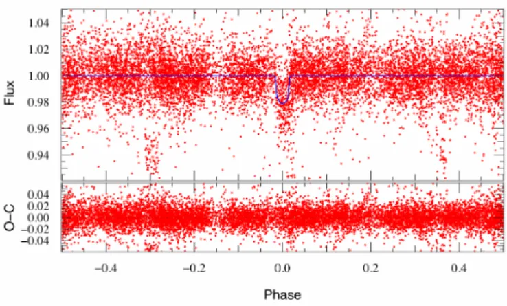
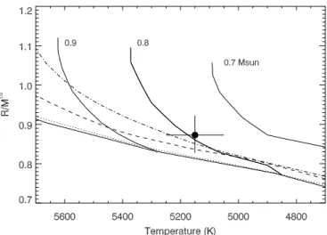
Fig. 1. Phased WASP-South photometry, of two seasons, and residuals. R band model superimposed.
bital planes with respect to the stellar rotation, some even on retrograde orbits (H´ebrard et al. 2008; Winn et al. 2009; Narita et al. 2009; Anderson et al. 2010; Queloz et al. 2010). The study of this angle’s distribution is being used to distinguish the pro-cesses through which hot Jupiters have arrived at their current orbits (Triaud et al. 2010; Winn et al. 2010a; Morton & Johnson 2010).
All this gathered data helps developments in theoretical physics in regimes beforehand out of reach: intense heat transfer between hot and cold hemispheres (Guillot & Showman 2002) and on supersonic winds (Dobbs-Dixon et al. 2010) to name only two. The few detections of multi-planet systems in which at least one component is transiting can also informs us about the inte-rior structure (Batygin et al. 2009). Obviously the study of these special exoplanets is also shedding light on how planets form as well as on the evolution of their orbits with time. The hot Jupiters are thought to have experienced a migration to the star after their formation beyond the ice-line, be it through some an-gular moment exchange with the primordial protoplanetary disc (Lin et al. 1996), or via dynamical interactions and subsequent tidal friction (Fabrycky & Tremaine 2007; Nagasawa et al. 2008; Malmberg et al. 2010), an explanation now preferred to the pre-vious one. The history of that post formation evolution might hold a key to the understanding of the various processes that planetary systems are likely to experience and thus, shed a light on the events around the origin of our own Solar System.
In that light, we announce the discovery of a new transiting gas giant by the WASP consortium, in close proximity with its host star, another brick in the understanding of these objects.
2. Observations
The object, WASP-23, (1SWASP J064430.59-424542.5) is a K1V star with V=12.68 and was observed through two seasons of the WASP-South survey, located in Sutherland, South Africa, in a single camera field from 2006 October 13 to 2007 March 11 and from 2007 October 11 to 2008 March 11 representing 10 846 photometric measurements. The WASP-South instrument, part of the WASP survey is amply described in Pollacco et al. (2006). The Hunter algorithm (Cameron et al. 2007b) searched the data and found 11 partial transits with a period of 2.94 days and a depth of 1.7 % in both seasons (Fig. 1). It was classed for spec-troscopic follow-up. No rotational variability could be found in the photometric data, indicating slow rotation and few stellar spots.
Table 1. Stellar parameters of WASP-23 from spectroscopic analysis. Teff 5150 ± 100 K [Fe/H] −0.05 ± 0.13 log g 4.4 ± 0.2 [Mg/H] +0.15 ± 0.15 ξt 0.8 ± 0.2 km s−1 [Si/H] +0.03 ± 0.08 vmac 0.8 ± 0.3 km s−1 [Ca/H] +0.17 ± 0.16 vsin I 2.2 ± 0.3 km s−1 [Sc/H] +0.03 ± 0.12 [Ti/H] +0.18 ± 0.13 B-V 0.88 ± 0.05 [V/H] +0.34 ± 0.13 log R0 HK −4.68 ± 0.07 [Cr/H] +0.04 ± 0.10 SMW 0.32 ± 0.04 [Mn/H] +0.05 ± 0.15 [Co/H] +0.11 ± 0.15
log A(Li) <1.0 [Ni/H] −0.03 ± 0.12
Table 2. Limb darkening coefficients used (quadratic law)
Band ua ub Band ua ub
VHARPS 0.576 0.191 z 0.284 0.289
R 0.450 0.260 I+ z 0.325 0.275
The 1.2 m Euler Swiss telescope, in La Silla, Chile, estab-lished the planetary nature of the object by observing the pres-ence of a Doppler variation of semi-amplitude 145 m s−1 with the same period and epoch as the WASP-South photometry. Observations started on 2008 August 31 and were pursued until 2010 April 08 totalling 38 radial velocity measurements (Fig. 2), each of 30 minute exposure.
A photometric timeseries was acquired with the cam-era mounted on the Euler telescope, in the z-band on 2008 December 13. We gathered 254 measurements and confirmed the reality of the photometric signal discovered by WASP-South (Fig. 3). In addition we gathered another 215 measurement in the zband during transit with the Faulkes South Telescope on 2009 September 27. We observed a third transit on 2010 February 7, with Euler, collecting 193 datapoints in the R-band filter (Fig. 3). Two further transits were observed during December 2010 using the newly built 60 cm TRAPPIST robotic telescope (Gillon et al. 2011), also located in La Silla, was finally added to this analysis (Fig. 4).
Under ESO proposal 084.C-0185 we observed with the spec-trograph HARPS, mounted on the ESO 3.6m telescope, at La Silla, Chile, obtaining 35 spectra between 2009 December 18 and 2010 February 9. 28 spectra at a mean cadence of roughly 600s were acquired on the first night, 14 of which are positioned while the planet transits (Fig. 2 & 3). The others were observed a few months later because of scheduling contraints and have exposure times of 1200s.
3. Data Analysis
3.1. the Euler z-band transit
The transit was observed in the z-band, on 2008 December 12, from 2h15 to 7h35 UTC using the Euler camera. The z-band fil-ter was used to minimise the impact of stellar limb-darkening on the deduced system parameters. The images were 2 × 2 binned to improve the duty cycle of the observations, resulting in a pixel scale of 0.7 arcsec. 254 exposures were acquired during the run, with an exposure time ranging from 45s to 60s. Two outliers were removed for the analysis. To keep a good spatial sampling while minimising the impact of interpixel sensitivity
inhomo-−200 −100 0 100 200 −0.4 −0.2 0.0 0.2 0.4 −40 −20 0 20 40 −0.10 −0.05 0.00 0.05 0.10 0.15 −0.4 −0.2 0.0 0.2 0.4 7.5 7.6 7.7 7.8 Radial Velocities (m.s −1 ) O−C (m.s −1 )
FWHM & Bis Span (km.s
−1 ) Phase . . . .
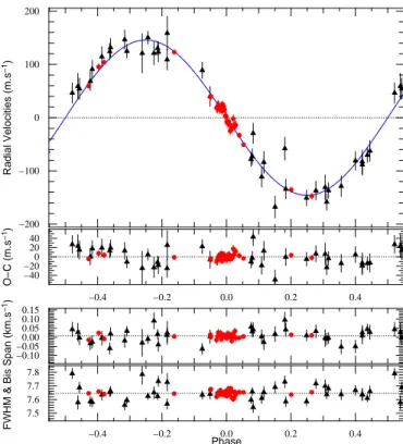
Fig. 2. Black triangles: CORALIE data; red discs: HARPS data. top: radial velocities with model superimposed, and residuals (both in m s−1), as a function of orbital phase. Added are the
1 σ error bars. bottom: Phased bisector span and FWHM (both in km s−1). The HARPS data has been translated to have its mean
correspond to the CORALIE data.
geneity and seeing variations, the telescope was heavily defo-cused: the mean profile width was 4.8 ± 0.2 arcsec. Airmass de-creased from 1.43 to 1.03 then raised to 1.09.
After a standard pre-reduction, stellar fluxes were extracted using the IRAF1version of the DAOPHOT aperture photometry
software (Stetson 1987). After a careful selection of reference stars, we subtracted a linear fit from the differential magnitudes as a function of airmass to correct for the different colour depen-dance of the extinction for the target and comparison stars. The linear fit was calculated from the out-of-transit (OOT) data and applied to all the data. The corresponding fluxes were then nor-malised using the OOT part of the photometry. Fig. 3 shows the resulting timeseries. The OOT rms is 2.2 mmag for a mean time sampling of 75s. Comparing this OOT rms to the one obtained after binning the data per 25 minutes (a duration comparable to the one of the ingress/egress) as described by Gillon et al. (2006) indicates the presence of a correlated noise of ∼ 600 ppm in the photometry.
3.2. the Euler R-band transit
A similar reduction was operated on the transit of 2010 February 7. After outlier rejection, we were left with 183 images of a mean sampling time of 63s. In this instance the telescope was not de-focused; the mean profile width was 2.3 arcsec. Transparency
1 IRAF is distributed by the National Optical Astronomy
Observatory, which is operated by the Association of Universities for Research in Astronomy, Inc., under cooperative agreement with the National Science Foundation
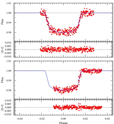
−20 −10 0 10 20 −0.04 −0.02 0.00 0.02 0.04 −20 −10 0 10 20 O − C (m.s − 1) Radial Velocities (m.s − 1) . . . . 0.98 0.99 1.00 1.01 −0.010 −0.005 0.000 0.005 0.010 0.98 0.99 1.00 1.01 −0.04 −0.02 0.00 0.02 0.04 −0.010 −0.005 0.000 0.005 0.010 Phase Flux O − C Flux O − C . . . . 0.98 0.99 1.00 1.01 −0.04 −0.02 0.00 0.02 0.04 −0.010 −0.005 0.000 0.005 0.010 Flux O − C Phase . . . . HARPS Euler z band Euler R band FTS z band
Fig. 3. HARPS radial velocity data corrected for the reflex Doppler motion due to the planet and model of the Rossiter-McLaughlin effect with residuals. Then three photometric transit as indicated, the best model and residuals. All are presented as a function of the orbital phase.
was good and airmass ranged from 1.03 to 2.22. Five stars were used as reference totalling a comparative flux 4.2 times that of the target. We observe some correlated noise here too, of ∼ 600 ppm in the photometry. The photometry is shown on Fig. 3.
0.98 0.99 1.00 1.01 −0.010 −0.005 0.000 0.005 0.010 0.98 0.99 1.00 1.01 −0.04 −0.02 0.00 0.02 0.04 −0.010 −0.005 0.000 0.005 0.010 . . . . . . . . Flux O−C Flux O−C Phase
Fig. 4. The two I + z band timeseries observed by TRAPPIST, with best model overplotted.
3.3. the FTS z-band transit
An additional transit of WASP-23b was obtained with the LCOGT22.0 m Faulkes Telescope South (FTS) at Siding Spring
Observatory, Australia on the night of 2009 September 27. Observations took place between 15:30 UTC and 19:00 UTC and the airmass decreased throughout from 1.9 at the start to 1.1. The em03 Merope camera was used with a 2 × 2 binning mode giving a field of view of 50 × 50 and a pixel scale of
0.278 arcsec/pixel. The data were taken through a Pan-STARRS-zfilter and the telescope was defocussed to prevent saturation and allow longer 35 sec exposure times to be used.
The data were pre-processed in the standard manner to perform the debiassing, dark subtraction and flatfielding steps. Aperture photometry was performed using DAOPHOT within the IRAF environment using a 10 pixel radius aperture and the differential photometry was performed relative to 14 comparison stars that were within the FTN field of view.
During the course of the FTS observations, we detected a& 0.55 mag deep flat-bottomed partial eclipse on a nearby (∼ 109 arcsec) star (USNO-B1.0 0472-0093932, α = 06h44037.6300 δ = −42◦45013.500) appears to be an eclipsing binary. A cursory
search of the WASP archive indicates that it is has an ephemeris of HJD(Min I)= 2454021.573377E + 1.421933 days with an eclipse depth of ∼ 0.75 mag.
3.4. the TRAPPIST I+ z band transits
A complete and a partial transit of WASP-23 were also observed with the robotic 60cm telescope TRAPPIST3) (Gillon et al.
2011). Located at La Silla ESO observatory (Chile), TRAPPIST is equipped with a 2K × 2K Fairchild 3041 CCD camera that has
2 http://lcogt.net
3 http://arachnos.astro.ulg.ac.be/Sci/Trappist
a 22’ × 22’ field of view (pixel scale= 0.64”/pixel). The transits of WASP-23 were observed on the nights of 2010 December 21 and 30. The sky conditions were clear. We used the 1x2 MHz out mode with 1 × 1 binning, resulting in a typical read-out + overhead time and read noise of 8.2 s and 13.5 e−, re-spectively. The integration time was 35s for both nights. We ob-served through a special ‘I+z’ filter that has a transmittance of zero below 700nm, and > 90% from 750nm to beyond 1100nm. The telescope was defocused to average pixel-to-pixel sensitivity variations and to optimize the duty cycle, resulting in a typical full width at half-maximum of the stellar images of ∼5.2 pixels (∼3.3”). The positions of the stars on the chip were maintained to within a few pixels over the course of the two runs, thanks to the ‘software guiding’ system that derives regularly an astro-metric solution on the most recently acquired image and sends pointing corrections to the mount if needed. After a standard pre-reduction (bias, dark, flatfield), the stellar fluxes were extracted from the images using the IRAF/DAOPHOT aperture photometry software (Stetson 1987). Several sets of reduction parameters were tested, and we kept the one giving the most precise pho-tometry for the stars of brightness similar to WASP-23. After a careful selection of reference stars, differential photometry was obtained. The data is shows in figure 4.
3.5. the spectral analysis
A total of 26 individual CORALIE spectra of WASP-23 were co-added to produce a single spectrum with a typical S/N of around 50:1. The standard pipeline reduction products were used in the analysis.
The analysis was performed using the methods given in Gillon et al. (2009). The Hαline was used to determine the
ef-fective temperature (Teff), while the Na i D and Mg i b lines
were used as surface gravity (log g) diagnostics. The parameters obtained from the analysis are listed in Table 1. The elemen-tal abundances were determined from equivalent width measure-ments of several clean and unblended lines. A value for micro-turbulence (ξt) of 0.8 km s−1 was determined from Fe i using
Magain (1984) method. The quoted error estimates include that given by the uncertainties in Teff, log g and ξt, as well as the
scat-ter due to measurement and atomic data uncertainties.
The projected stellar rotation velocity (v sin I )4 was deter-mined by fitting the profiles of several unblended Fe i lines. Because the value of v sin I was paramount to the model fitting, we used the combined HARPS spectra. A value for macrotur-bulence (vmac) of 0.8 ± 0.3 km s−1was assumed, based on work
by Bruntt et al. (2010) and an instrumental FWHM of 0.060Å, determined from the telluric lines around 6300Å. A best fitting value of v sin I = 2.2 ± 0.3 km s−1was obtained. Using a macro-turbulence based on the tabulation by Gray (2008) of 1.2 km s−1
we obtain the same result for v sin I showing its robustness. The HARPS spectra show that there is weak emission in the cores of the Calcium H & K lines. Activity levels on the star are estimated by means of the log R0
HK(Noyes et al. 1984; Santos
et al. 2000; Boisse et al. 2009) and obtained using a B − V = 0.88 ± 0.05 estimated from the effective temperature. The Mount Wilson index, SMWis also given.
4 We make a distinction between v sin I and V sin I. The latter is a result of the Rossiter-McLaughlin fit. i being traditionally the planet’s orbital inclination, we denote by I, the inclination of the stellar spin axis
3.6. the RV extraction
The spectroscopic data were reduced using the online Data Reduction Software (DRS) for the HARPS instrument. The ra-dial velocity information was obtained by removing the instru-mental blaze function and cross-correlating each spectrum with a K5 mask. This correlation is compared with the Th-Ar spec-trum acting as a reference; see Baranne et al. (1996) & Pepe et al. (2002) for details. Recently the DRS was shown to achieve remarkable precision (Mayor et al. 2009) thanks to a revision of the reference lines for Thorium and Argon by Lovis & Pepe (2007). A similar software package is used for CORALIE data. A resolving power R = 110 000 for HARPS yields a cross-correlation function (CCF) binned in 0.25 km s−1 increments, while for CORALIE, with a lower resolution of 50 000, we used 0.5 km s−1. The CCF window was adapted to be three times the size of the full width at half maximum (FWHM) of the CCF.
1 σ error bars on individual data points were estimated from photon noise alone. HARPS is stable on the long term within 1 m s−1and CORALIE to better than 5 m s−1. These are smaller
than our individual error bars and thus have not been taken into account.
The absence of a variation in bisector span correlated with the phase, or of a variation of the FWHM, indicate that the pho-tometric and spectroscopic signals are indeed those of a planet. For comparison we invite the reader to look at Santos et al. (2002), on HD 41004 for which it has been proven a blend by a star and its brown dwarf companion was causing a spectro-scopic Doppler shift similar to that of a planet on a foreground object.
4. Modelling the data
The data was fitted using a Markov Chain Monte-Carlo (MCMC) method. A code allowing to combine both photome-try and spectroscopy has been developed. It has been used in several occasions (Bouchy et al. 2008; Gillon et al. 2008) and is described in length in Triaud et al. (2009). It is similar to those presented in Cameron et al. (2007a). The code uses a common set of free parameters from which physical parameters can be derived to construct models for the photometric and the spectro-scopic signal.
4.1. parameter choice
Free parameters used are: P the period of the object, T0the
mid-transit time, D the depth of the mid-transit, W its width, b the impact parameter, K the semi-amplitude of the Doppler reflex motion by the star. To fit the Rossiter-McLaughlin, we use √V sin I cos β and √V sin I sin β where V sin I is the projected stellar rota-tion and β the projected spin-orbit angle. Trying to estimate if the orbit is eccentric we used √ecos ω and √esin ω where e is the eccentricity and ω is the argument of the periastron. In ad-dition we at times added ˙γ , a radial-velocity drift with time, in order to assess the presence of an additional body in the system. In addition to these we need to fit one normalisation factor for each photometric dataset (5 in our case) and 2 γ velocities for the radial velocities, one for each set. We used Gaussian priors to draw randomly each parameter.
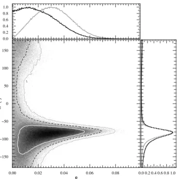
We decided to use √ecos ω & √esin ω as free param-eters instead of the more traditional e cos ω & e sin ω be-cause this would amount to impose a prior proportional to e2 as noted in Ford (2006). Figure 5 shows the difference be-tween both runs. Having √ecos ω & √esin ω makes the
0.0 0.2 0.4 0.6 0.8 1.0 0.00 0.02 0.04 0.06 0.08 −150 −100 −50 0 50 100 150 0.0 0.2 0.4 0.6 0.8 1.0 ω0 ( o) e . . . .
Fig. 5. In the central box we have the a posteriori probabil-ity densprobabil-ity function for e and ω, resulting from a chain using √
ecos ω & √esin ω as free parameters (from which e and ω were computed to fit an eccentric model to the data). The white contour marks the 68.27 % confidence region. The black dashed contour shows the 95.45 %, and the black dotted contour is the 99.73 %. Marginalised distributions are also shown as black his-tograms in side boxes, normalised to the mode. Grey hishis-tograms in the side boxes show the same fit but instead having e cos ω & esin ω as jump parameters.
eccentricity less biased towards high values. We therefore made a similar change to another pair of variables, making √
V sin I cos β and √
V sin I sin β as free parameters rather than using V sin I cos β and V sin I sin β. Checks for these were also conducted and validated our choice of jump param-eters.
4.2. models & hypotheses
We used models from Mandel & Agol (2002) to fit the photo-metric transit and from Gim´enez (2006) to adjust the Rossiter-McLaughlin effect as well as a classical Keplerian model for the orbital variation in the radial velocities. Limb darkening coe ffi-cients for the quadratic law were extracted from Claret (2000, 2004) for the photometry. To fit the Rossiter-McLaughlin effect we used coefficients specially made from HARPS’s spectral re-sponse, that were presented in Triaud et al. (2009). Table 2 shows the values we adopted.
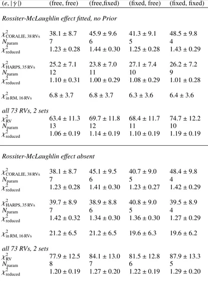
These models are compared to the data using a χ2statistics. A first series of four chains was run and led to a stellar density estimate. This values have been used to determine a stellar mass from evolutionary models by Girardi et al. (2000) as described in Hebb et al. (2009) using the metallicity and temperature deter-mined in the spectral analysis and the stellar density from fitting the photometric transit. By interpolating between the tracks we find M? = 0.79+0.13−0.12M (Fig. 6). This stellar mass was inserted
as a prior in a new series of chains. The stellar age could not be constrained but is likely old; the star sits above the 10 Gyr
Fig. 6. Modified Hertzprung-Russell diagram comparing the stellar density and temperature of WASP-23 to theoretical stel-lar evolutionary tracks interpolated for a metallicity of [M/H] = −0.05. The star sits just above the 10 Gyr tracks (dashdotted line). Other tracks are: 0.1 Gyr (solid), 1 Gyr (dotted), 5 Gyr (dashed). Models are by Girardi et al. (2000)
isochrone. This first series of chains also allowed the quantifi-cation of the correlated noise in the data which is accounted for in the following chains by increasing individual error bars. This allows us to place more credible error bars for parameters deter-mined by the photometry.
Two families of chains, each with 2 000 000 random steps, were run. A family consist of four chains with varying hypothe-ses:
– eccentricity and RV drift let free; – no eccentricity but RV drift let free; – no RV drift but eccentricity let free; – no eccentricity and no RV drift .
We ran two families, one with the Rossiter-McLaughlin ef-fect let free and one without. Hence from these 8 chains we tested for the presence of a linear trend in the radial velocities, for the detection of eccentricity and the detection of the Rossiter-McLaughlin effect.
5. Results
We have computed 8 different chains, each with different hy-potheses. All chains agree in their results within each others’ error bars in their common parameters, giving strong evidence that indeed they have converged to the solution. Results were extracted from each chain and their comparison with each oth-ers lead to the final results here presented. This comparison, available for its most interesting parts in the appendices, made us choose a circular, non drifting model for the radial veloc-ity. WASP-23b’s parameters are extracted by taking the mode of the marginalised distributions computed by the Markov chains. When two clear separated mode appear, each is estimated and er-rors bars calculated (see Fig. 8). Error bars are computed by tak-ing the 68.27%, 95.45% and 99.73% marginalised confidence re-gions in the a posteriori probability density distribution. Models using eccentricity and a drift as free floating parameters are use-ful to place upper constraints on these parameters. Results are
0.0 0.2 0.4 0.6 0.8 1.0 −50 0 50 0 1 2 3 4 5 6 0.0 0.2 0.4 0.6 0.8 1.0 V sin I (km.s −1 ) β (o) . . . .
Fig. 7. Same legend as on Fig. 5 but here showing V sin I and β, for a circular, non drifting orbital solution using no prior on V sin I.
presented in Table 3. The final reduced χ2for the radial veloci-ties, both for CORALIE and HARPS observations, is consistent with 1. We therefore saw no need to add any additional terms to our error bars.
WASP-23b, therefore, is a 0.88 MJplanet with a 0.96 RJ
ra-dius on a 2.94 day orbit, placing it among the normally sized hot Jupiter planets. We can reasonably estimate upper limits on the eccentricity and RV trend at the 99% exclusion level, from the chains that had these as free parameters. Thus we find that e< 0.062 & | ˙γ | < 30 m s−1yr−1.
Using no prior, we have detected a radial velocity anomaly compatible with the expected location and shape of the Rossiter-McLaughlin (χ2 changes from 19.6 ± 6.2 to 6.4 ± 3.6 for the
14 data points positioned during transit and one on either side). We detected this effect to a confidence of 3.2 σ from a simple Keplerian model. We see a degeneracy arising between β, V sin I & b, the impact parameter: V sin I grows to extremely large val-ues (up to 60 km s−1, Fig. 7) by forcing β to severely misaligned
solution and b closer to an equatorial transit.
Because of the non physicality of such result for V sin I we will have to resort to the use of some prior in order to constrain the space within which the MCMC can explore. We do this by imposing a Bayesian penalty on χ2. This additional analysis is presented in the discussion.
Our chains indicate that the effect is mostly symmetrical with respect to the centre of transit (see Fig. 7), and that we can ex-clude a retrograde orbit.
6. Discussion
Figure 7 shows unambiguously that we have a strong degener-acy between β and V sin I. This is a known problem notably reported already in Narita et al. (2010) & Triaud et al. (2010). Spectral line analysis (section 3.5) showed that the projected stellar rotation velocity v sin I= 2.2 ± 0.3 km s−1. From figure 7
−50 0 50 0.0 0.2 0.4 0.6 0.8 1.0 0.0 0.2 0.4 0.6 0.8 1.0 0 1 2 3 . . . . V sin I (km.s − 1) β (o) 0.0 0.1 0.2 0.3 0.4 0.5 0.0 0.2 0.4 0.6 0.8 1.0 0 1 2 3 . . . . b (Rs) −50 0 50 0.0 0.2 0.4 0.6 0.8 1.0 0.0 0.1 0.2 0.3 0.4 0.5 . . . . b (Rs) . . . . 0.0 0.2 0.4 0.6 0.8 1.0 −50 0 50 0 1 2 3 0.0 0.2 0.4 0.6 0.8 1.0 . . . . −50 0 50 0.0 0.1 0.2 0.3 0.4 0.5 0.0 0.2 0.4 0.6 0.8 1.0 . . . . β ( o) b (Rs) 0.0 0.2 0.4 0.6 0.8 1.0 0.0 0.1 0.2 0.3 0.4 0.5 0 1 2 3 . . . . b (Rs) V sin I (km s − 1)
Fig. 8. Square boxes present the a posteriori probability density functions for V sin I, β and impact parameter b, from which we extract our results. The white contour marks the 68.27 % confidence region. The black dashed contour shows the 95.45 %, and the black dotted contour is the 99.73 %. Marginalised distributions are also shown as black histograms in side boxes, normalised to the mode. On top right, in red, we have the results for a circular, non drifting solution with use of a prior of v = 1.35 ± 0.20 km s−1.
On bottom left, in blue, we show a circular, non drifting solution with the application of a prior of v sin I= 2.2 ± 0.3 km s−1. Grey histograms in V sin I and β show results in the photometry limited runs; for b we plotted the resulting distribution by fitting the photometry alone without the Rossiter-McLaughlin effect.
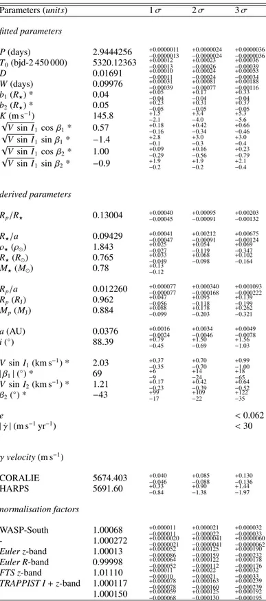
Table 3. Fitted and derived parameters for WASP-23 & WASP-23b with their error bars for confidence intervals of 68.27%, 95.45% and 99.73%. For asterisked parameters, please refer to the text. Underscripted 1 and 2 are for showing 2 distinct solutions for the same parameter Parameters (units) 1 σ 2 σ 3 σ fitted parameters P(days) 2.9444256 +0.0000011−0.0000013 +0.0000024−0.0000024 +0.0000036−0.0000036 T0(bjd-2 450 000) 5320.12363 +0.00012−0.00013 +0.00023−0.00026 +0.00036−0.00039 D 0.01691 +0.00010−0.00011 +0.00024−0.00024 +0.00053−0.00034 W(days) 0.09976 +0.00031−0.00039 +0.00081−0.00077 +0.00188−0.00116 b1(R?) * 0.04 +0.05−0.04 +0.17−0.04 +0.33−0.04 b2(R?) * 0.05 +0.23−0.05 +0.31−0.05 +0.37−0.05 K(m s−1) 145.8 +1.5 −2.1 +3.4−4.0 +5.3−5.6 √ V sin I1 cos β1* 0.57 +0.18−0.16 +0.42−0.34 +0.66−0.46 √ V sin I1 sin β1* −1.4 +2.8−0.1 +3.0−0.3 +3.0−0.4 √ V sin I1 cos β2* 1.00 +0.09−0.29 +0.16−0.56 +0.23−0.79 √ V sin I1 sin β2* −0.9 +1.9−0.2 +1.9−0.2 +2.1−0.4 derived parameters Rp/R? 0.13004 +0.00040−0.00045 +0.00095−0.00091 +0.00203−0.00132 R?/a 0.09429 +0.00041−0.00047 +0.00212−0.00091 +0.00675−0.00124 ρ?(ρ ) 1.843 +0.025−0.027 +0.054−0.119 +0.069−0.347 R?(R ) 0.765 +0.033−0.049 +0.068−0.098 +0.102−0.164 M?(M ) 0.78 +0.13−0.12 Rp/a 0.012260 +0.000077−0.000077 +0.000340−0.000168 +0.001093−0.000222 Rp(RJ) 0.962 +0.047−0.056 +0.095−0.118 +0.139−0.199 Mp(MJ) 0.884 +0.088−0.099 +0.178−0.203 +0.262−0.321 a(AU) 0.0376 +0.0016−0.0024 +0.0034−0.0046 +0.0049−0.0078 i(◦ ) 88.39 +0.79−0.45 +1.50−0.69 +1.56−1.03 V sin I1(km s−1) * 2.03 +0.37−0.35 +0.70−0.70 +0.99−1.00 |β1| (◦) * 69 +6−9 +14−24 +18−65 V sin I2(km s−1) * 1.21 +0.17−0.23 +0.42−0.39 +0.64−0.52 β2(◦) * −43 +99−17 +109−22 +122−35 e < 0.062 | ˙γ | (m s−1yr−1) < 30 γ velocity (m s−1) CORALIE 5674.403 +0.040−0.046 +0.085−0.088 +0.130−0.136 HARPS 5691.60 +0.33−0.84 +0.90−1.38 +1.44−1.97 normalisation factors WASP-South 1.00068 +0.000011−0.000011 +0.000021−0.000022 +0.000032−0.000033 - 1.000272 +0.0000020−0.0000021 +0.0000041−0.0000041 +0.0000060−0.0000062 Euler z-band 1.00013 +0.000052−0.000086 +0.000125−0.000159 +0.000190−0.000232 Euler R-band 0.99998 +0.000064−0.000052 +0.000122−0.000112 +0.000178−0.000176 FTS z-band 1.01110 +0.00011−0.00010 +0.00022−0.00021 +0.00032−0.00033 TRAPPIST I+ z-band 1.000117 +0.000078−0.000078 +0.000163−0.000160 +0.000239−0.000239 1.000150 +0.000059−0.000068 +0.000125−0.000130 +0.000192−0.000195
we observe that a V sin I at such a value would lead to a severely misaligned orbit. This is confirmed when running the MCMC for an additional family of chains using this value of v sin I as a prior on V sin I.
We call this our solution 1: we obtain two modes for β sym-metrically opposite to each other (see Fig. 8, bottom left corner). We therefore choose to denote this result by its absolute value as | β1|= 69◦+6−9; V sin I1= 2.03+0.37−0.35 km s−1. Impact parameter
b1= 0.04±0.05 R?. This prior choice makes the detection of the
Rossiter-McLaughlin effect close to 7.5 σ.
Before claiming an additional misaligned planet, one around a cool star (thus a strong exception to Winn et al. (2010a)), we have searched for another independent estimate of stellar rota-tion.
From spectral analysis, we obtained a value quantifying emission in the Calcium II lines expressed in the form of log R0HK = −4.68 ± 0.07. This value can be used as an indi-rect measurement of the true stellar rotation period. We used two methods, by Noyes et al. (1984), finding 28.6+5.3−5.3days and a more recent estimate by Mamajek & Hillenbrand (2008) and got the value 28.2+4.4−5.3days in very good agreement with the pre-vious. Using the distribution of R?from our MCMC chains, we transformed these values in the equatorial rotation v obtaining 1.30+0.24−0.19and 1.35+0.28−0.20km s−1respectively. Combining both we have our new prior that we included as 1.35 ± 0.20 km s−1into a new series of four chains. Results from these indicate that the planet is most likely on an aligned orbit, but error bars remain large.
We call these results, our solution 2: we only have one large range of values for the projected spin-orbit angle: β2= −43◦+99−17.
V sin I2 = 1.21+0.17−0.23km s −1and b
2= 0.05+0.23−0.05R?. Here too, the
detection of the Rossiter-McLaughlin is more secure, climbing to a value close to 7 σ.
In order to test our results we simulated whether an infinitely precise photometry would help discriminate between our differ-ing solutions for β since the parameter b, for example, is in-fluenced by the adjustment of the Rossiter-McLaughlin model. We therefore removed the Rossiter-McLaughlin effect and ran a chain only using photometry on the transit parameters stick-ing with the non driftstick-ing, non eccentric model. Havstick-ing photom-etry as the sole influence on the impact parameter, one finds b = 0.28+0.08−0.14R?. The value found for b1and b2are not at odds
with this value. We fixed the parameters controlled by photome-try to the best found values (ie. b= 0.28) and ran an additional three chains. Those three ”photometry limited” chains had the following differences:
– no imposed prior;
– a prior of 2.2 ± 0.3 km s−1;
– a prior of 1.35 ± 0.20 km s−1.
Refer to figure 8 to see the resulting probability distributions (grey histograms). By fixing all parameters to the values that can be determined by photometry alone and letting free again all re-maining parameters, we see some changes in the posterior prob-ability distributions (see grey histograms on Fig. 8). The distri-bution of V sin I1is shifted to lower values, while that of β1,
al-though still bimodal, is less so. V sin I2is left almost unchanged,
but β2 is more confined around 0. This shows what effect our
poorly constrained impact parameter induces on our fit, but this also indicates that, unless a new transit finds a higher value of b, even an infinitely precise photometry would not help lifting entirely the degeneracy between β and V sin I for b < 0.28 R?.
The measurement of the projected spin-orbit angle β is mostly affected by the low amplitude of the signal and in part by the poorly determined impact parameter, which, floating to small values, helps create a degeneracy between small β, small V sin I and high β, high V sin I.
7. Conclusions
After the analysis of more than 4 years of photometric and spec-troscopic data, we confidently conclude that we have detected a typical hot Jupiter around the K1V star called WASP-23. The analysis was made a bit more arduous because of degeneracy arising when adjusting for the Rossiter-McLaughlin effect. A to-tal of 19 Markov chains were used to derive our conclusions.
Despite the slow rotation and likely old age of the star, we manage to detect the Rossiter-McLaughlin effect, which is of a similar amplitude to that of WASP-2b (Triaud et al. 2010) and of a similar signal to noise to detections like that on Hat-P-11b (Winn et al. 2010b; Hirano et al. 2010a). Imposing priors on V sin I increases our detection level but seriously affects the posterior probability distribution (see Fig. 7 & 8) and thus our re-sults and our possible interpretations. This mostly come from the difference between our two priors, which are 2.7 σ away from each other although our value of v sin I= 2.2 ± 0.3 km s−1 (so-lution 1) should be seen as a lower value, while v= 1.35 ± 0.20 km s−1(solution 2) is more of an upper value.
There is strong evidence that for stars colder than 6250 K, planets tend to have a high a priori probability to be aligned with the stellar spin (Winn et al. 2010a). This then would support our solution 2 and thus imply that the spectral line broadening method is not accurate enough to determine v sin I. This would demonstrate that there is a potential difficulty with the estimation of v sin I and its use as a prior. But solution 2 is not without its problems either since the determination of the stellar rotation from activity indices could be altered by the presence of a nearby hot Jupiter and long term magnetic cycles.
To resolve WASP-23b’s spin orbit angle, one has several options. One could acquire more and better photometry. If b were to be found small, then the degeneracy will not be lifted, but the larger it is found, the more likely the system will be aligned. Additionally, further observations might be needed of the Rossiter-McLaughlin. There is also a possibility that the cur-rent data is enough as one could use the Doppler shadow method pioneered in Cameron et al. (2010) and Miller et al. (2010). This method provides precise determinations of V sin I, β and b but works best for fast rotators and bright targets.
Either way, the resolution of our degenerate result is inter-esting. If solution 1 (prior on V sin I = 2.2 ± 0.3 km s−1) is
confirmed, we have a misaligned system around a cold star and a need to rectify the determination of stellar rotation from activ-ity levels. If solution 2 (prior on V sin I = 1.35 ± 0.20 km s−1)
is preferred, then we have probably and aligned system and one will know to be careful when using v sin I prior found by spec-tral line broadening.
We therefore recommend extreme caution when using priors as final results can entirely depend on those and a small initial systematic error can lead to dramatic changes in interpretation.
Nota Bene We used the UTC time standard and Barycentric Julian Dates in our analysis. Our results are using the equato-rial solar and jovian radii and masses from Allen’s Astrophysical Quantities.
Acknowledgements. The authors would like to acknowledge the use of ADS and
of Simbad but mostly the help and the kind attention of the ESO staff at La Silla which with its (now gone and much regretted) completos insured a good and stable supply of energy during the long observing nights. The work is supported by the Swiss Fond National de Recherche Scientifique. TRAPPIST is a project funded by the Belgian Fund for Scientific Research (FNRS) with the partici-pation of the Swiss National Science Fundation (SNF). M. Gillon and E. Jehin are FNRS Research Associate. We also thank R. Heller for providing a copy of Holt’s 1893 paper.
References
Anderson, D. R., Hellier, C., Gillon, M., et al. 2010, ApJ, 709, 159 Bakos, G., Noyes, R. W., Kov´acs, G., et al. 2004, PASP, 116, 266 Baranne, A., Queloz, D., Mayor, M., et al. 1996, A&A, 119, 373 Batygin, K., Bodenheimer, P., & Laughlin, G. 2009, ApJ, 704, L49 Boisse, I., Moutou, C., Vidal-Madjar, A., et al. 2009, A&A, 495, 959 Bouchy, F., Queloz, D., Deleuil, M., et al. 2008, A&A, 482, L25 Bruntt, H., Bedding, T. R., Quirion, P.-O., et al. 2010, MNRAS, 405, 1907 Cameron, A. C., Bouchy, F., H´ebrard, G., et al. 2007a, MNRAS, 375, 951 Cameron, A. C., Bruce, V. A., Miller, G. R. M., Triaud, A. H. M. J., & Queloz,
D. 2010, MNRAS, 180
Cameron, A. C., Wilson, D. M., West, R. G., et al. 2007b, MNRAS, 380, 1230 Charbonneau, D., Brown, T. M., Latham, D. W., & Mayor, M. 2000, ApJ, 529,
L45
Claret, A. 2000, A&A, 363, 1081 Claret, A. 2004, A&A, 428, 1001
Dobbs-Dixon, I., Cumming, A., & Lin, D. N. C. 2010, ApJ, 710, 1395 Fabrycky, D. & Tremaine, S. 2007, ApJ, 669, 1298
Ford, E. B. 2006, ApJ, 642, 505
Gillon, M., Anderson, D. R., Triaud, A. H. M. J., et al. 2009, A&A, 501, 785 Gillon, M., Jehin, E., Magain, P., et al. 2011, eprint arXiv, 1101, 5807 Gillon, M., Pont, F., Moutou, C., et al. 2006, A&A, 459, 249 Gillon, M., Triaud, A. H. M. J., Mayor, M., et al. 2008, A&A, 485, 871 Gim´enez, A. 2006, ApJ, 650, 408
Girardi, L., Bressan, A., Bertelli, G., & Chiosi, C. 2000, A&AS, 141, 371 Gray, D. F. 2008, The Observation and Analysis of Stellar Photospheres Guillot, T. & Showman, A. P. 2002, A&A, 385, 156
Hebb, L., Cameron, A. C., Loeillet, B., et al. 2009, ApJ, 693, 1920 H´ebrard, G., Bouchy, F., Pont, F., et al. 2008, A&A, 488, 763
Hirano, T., Narita, N., Shporer, A., et al. 2010a, eprint arXiv, 1009, 5677 Hirano, T., Suto, Y., Taruya, A., et al. 2010b, ApJ, 709, 458
Holt, J. 1893, Astronomy & Astrophysics, XII, 646
Lin, D. N. C., Bodenheimer, P., & Richardson, D. C. 1996, Nature, 380, 606 Lovis, C. & Pepe, F. 2007, A&A, 468, 1115
Magain, P. 1984, A&A, 134, 189
Malmberg, D., Davies, M. B., & Heggie, D. C. 2010, eprint arXiv, 1009, 4196 Mamajek, E. E. & Hillenbrand, L. A. 2008, ApJ, 687, 1264
Mandel, K. & Agol, E. 2002, ApJ, 580, L171
Mayor, M., Udry, S., Lovis, C., et al. 2009, A&A, 493, 639
McCullough, P. R., Stys, J. E., Valenti, J. A., et al. 2005, PASP, 117, 783 McLaughlin, D. B. 1924, ApJ, 60, 22
Miller, G. R. M., Cameron, A. C., Simpson, E. K., et al. 2010, arXiv, astro-ph.EP Morton, T. D. & Johnson, J. A. 2010, eprint arXiv, 1010, 4025
Nagasawa, M., Ida, S., & Bessho, T. 2008, ApJ, 678, 498
Narita, N., Hirano, T., Sanchis-Ojeda, R., et al. 2010, PASJ, 62, L61 Narita, N., Sato, B., Hirano, T., & Tamura, M. 2009, PASJ, 61, L35
Noyes, R. W., Weiss, N. O., & Vaughan, A. H. 1984, Astrophysical Journal, 287, 769
O’Donovan, F. T., Charbonneau, D., & Hillenbrand, L. 2006, 2007 AAS/AAPT Joint Meeting, 209, 1212
Ohta, Y., Taruya, A., & Suto, Y. 2005, ApJ, 622, 1118 Pepe, F., Mayor, M., Galland, F., et al. 2002, A&A, 388, 632
Pollacco, D. L., Skillen, I., Cameron, A. C., et al. 2006, PASP, 118, 1407 Queloz, D., Anderson, D., Cameron, A. C., et al. 2010, A&A, 517, L1 Queloz, D., Eggenberger, A., Mayor, M., et al. 2000, A&A, 359, L13 Rossiter, R. A. 1924, ApJ, 60, 15
Santos, N. C., Mayor, M., Naef, D., et al. 2000, A&A, 361, 265 Santos, N. C., Mayor, M., Naef, D., et al. 2002, A&A, 392, 215
Snellen, I. A. G., van der Burg, R. F. J., de Hoon, M. D. J., & Vuijsje, F. N. 2007, A&A, 476, 1357
Stetson, P. B. 1987, PASP, 99, 191
Triaud, A. H. M. J., Cameron, A. C., Queloz, D., et al. 2010, A&A, 524, 25 Triaud, A. H. M. J., Queloz, D., Bouchy, F., et al. 2009, A&A, 506, 377 Udalski, A., Kubiak, M., & Szymanski, M. 1997, Acta Astronomica, 47, 319 Winn, J. N., Fabrycky, D., Albrecht, S., & Johnson, J. A. 2010a, ApJ, 718, L145 Winn, J. N., Johnson, J. A., Albrecht, S., et al. 2009, ApJ, 703, L99
Winn, J. N., Johnson, J. A., Howard, A. W., et al. 2010b, ApJ, 723, L223
Appendix A: Comparisons between different chains.
In order to lighten the text, here are placed the results of the Markov Chains using various starting hypotheses and from which we estimated upper limits on eccentricity and long term radial velocity trends.
Table A.1 compares the results in χ2by instrument and
dur-ing the Rossiter-McLaughlin effect for eights chains. From this we concluded that the eccentric orbit model is compatible with the circular, that a drift that can be fitted is statistically indistin-guishable from zero, but that we detect an anomaly in the re-flex Doppler motion, corresponding to the location where the Rossiter-McLaughlin effect is expected.
Table A.2 explores the parameters issued from chains where the Rossiter-McLaughlin effect was fitted in order to make sense of the results and see their dependency on initial hypotheses.
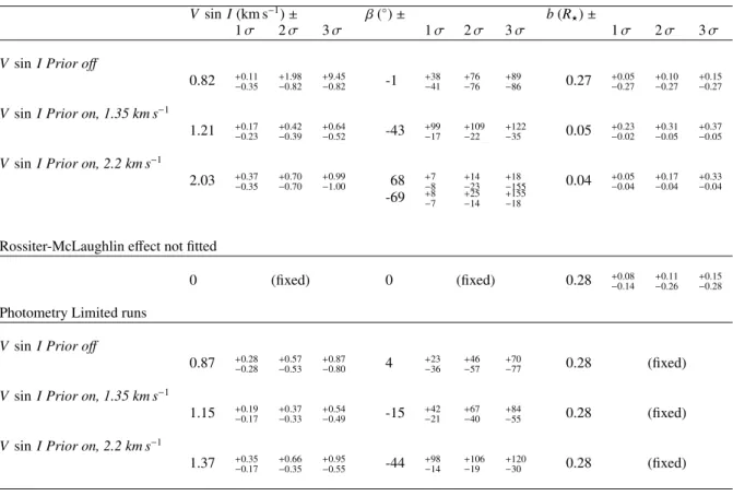
Table A.1. Here we compare the results in χ2by instrument and during the Rossiter-McLaughlin effect 2 different families of chains:
having no prior on V sin I, and not fitting the Rossiter-McLaughlin effect.
(e, | ˙γ |) (free, free) (free,fixed) (fixed, free) (fixed, fixed) Rossiter-McLaughlin effect fitted, no Prior
χ2 CORALIE, 38 RVs 38.1 ± 8.7 45.9 ± 9.6 41.3 ± 9.1 48.5 ± 9.8 Nparam 7 6 5 4 χ2 reduced 1.23 ± 0.28 1.44 ± 0.30 1.25 ± 0.28 1.43 ± 0.29 χ2 HARPS, 35 RVs 25.2 ± 7.1 23.8 ± 7.0 27.1 ± 7.4 26.2 ± 7.2 Nparam 12 11 10 9 χ2 reduced 1.10 ± 0.31 1.00 ± 0.29 1.08 ± 0.29 1.01 ± 0.28 χ2 in RM, 16 RVs 6.8 ± 3.7 6.8 ± 3.7 6.3 ± 3.6 6.4 ± 3.6 all 73 RVs, 2 sets χ2 RV 63.4 ± 11.3 69.7 ± 11.8 68.4 ± 11.7 74.7 ± 12.2 Nparam 13 12 11 10 χ2 reduced 1.06 ± 0.19 1.14 ± 0.19 1.10 ± 0.19 1.19 ± 0.19
Rossiter-McLaughlin effect absent χ2 CORALIE, 38 RVs 38.1 ± 8.7 45.1 ± 9.5 40.7 ± 9.0 48.4 ± 9.8 Nparam 7 6 5 4 χ2 reduced 1.23 ± 0.28 1.41 ± 0.30 1.23 ± 0.27 1.42 ± 0.29 χ2 HARPS, 35 RVs 39.7 ± 8.9 38.9 ± 8.8 40.8 ± 9.0 39.5 ± 8.9 Nparam 7 6 5 4 χ2 reduced 1.42 ± 0.32 1.34 ± 0.30 1.36 ± 0.30 1.27 ± 0.29 χ2 in RM, 16 RVs 21.2 ± 6.5 21.2 ± 6.5 19.6 ± 6.3 19.6 ± 6.2 all 73 RVs, 2 sets χ2 RV 77.9 ± 12.5 84.1 ± 13.0 81.5 ± 12.8 87.9 ± 13.3 Nparam 8 7 6 5 χ2 reduced 1.20 ± 0.19 1.27 ± 0.20 1.22 ± 0.19 1.29 ± 0.20
Table A.2. Here are presented the results from various Markov chains of the three parameters which control the shape of the Rossiter-McLaughlin effect. These are for circular non drifting orbital solutions.
Vsin I (km s−1) ± β (◦
) ± b(R?) ±
1 σ 2 σ 3 σ 1 σ 2 σ 3 σ 1 σ 2 σ 3 σ
V sin I Prior off
0.82 +0.11−0.35 +1.98−0.82 +9.45−0.82 -1 +38−41 +76−76 +89−86 0.27 +0.05−0.27 +0.10−0.27 +0.15−0.27 V sin I Prior on, 1.35 km s−1
1.21 +0.17−0.23 +0.42−0.39 +0.64−0.52 -43 +99−17 +109−22 +122−35 0.05 +0.23−0.02 +0.31−0.05 +0.37−0.05 V sin I Prior on, 2.2 km s−1
2.03 +0.37−0.35 +0.70−0.70 +0.99−1.00 68 +7−8 +14−23 +18−155 0.04 +0.05−0.04 +0.17−0.04 +0.33−0.04 -69 +8−7 +25−14 +155−18
Rossiter-McLaughlin effect not fitted
0 (fixed) 0 (fixed) 0.28 +0.08−0.14 +0.11−0.26 +0.15−0.28
Photometry Limited runs V sin I Prior off
0.87 +0.28−0.28 +0.57−0.53 +0.87−0.80 4 +23−36 +46−57 +70−77 0.28 (fixed) V sin I Prior on, 1.35 km s−1
1.15 +0.19−0.17 +0.37−0.33 +0.54−0.49 -15 +42−21 +67−40 +84−55 0.28 (fixed) V sin I Prior on, 2.2 km s−1
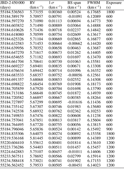
Table A.3. The HARPS data, comprising the Rossiter-McLaughlin effect. JBD-2 450 000 RV 1 σ BS span FWHM Exposure (days) (km s−1) (km s−1) (km s−1) (km s−1) (s) 55184.536563 5.73155 0.00360 0.00524 6.17685 1800 55184.589179 5.70957 0.00791 -0.01091 6.12089 600 55184.597270 5.71090 0.01113 0.00694 6.14773 500 55184.603832 5.71490 0.00889 0.03064 6.14888 600 55184.610626 5.71436 0.00718 0.02237 6.14842 600 55184.618080 5.70599 0.00754 0.02609 6.13617 600 55184.625326 5.71104 0.00669 0.02865 6.16877 600 55184.632583 5.71453 0.00664 -0.00662 6.14420 600 55184.639956 5.70352 0.00658 0.00463 6.13687 600 55184.647270 5.71617 0.00673 0.01262 6.14405 600 55184.654655 5.71182 0.00693 0.01697 6.13470 600 55184.661704 5.70641 0.00730 0.01063 6.15581 600 55184.669227 5.69401 0.00835 0.00671 6.13308 600 55184.676634 5.69442 0.00714 0.01096 6.16352 600 55184.683533 5.68357 0.00752 -0.00056 6.12561 600 55184.691357 5.68068 0.00853 0.02552 6.14308 600 55184.698822 5.68454 0.00769 0.01908 6.18173 600 55184.705859 5.67920 0.00704 0.01698 6.13790 600 55184.713186 5.66648 0.00745 0.01872 6.14939 600 55184.720582 5.66897 0.00667 0.00385 6.18264 600 55184.727897 5.67299 0.00695 -0.01616 6.11436 600 55184.735142 5.67307 0.00746 0.01983 6.15680 600 55184.742538 5.68932 0.00762 0.02362 6.10253 600 55184.749853 5.67476 0.00822 0.00608 6.11238 600 55184.757041 5.67851 0.00813 0.03817 6.15604 600 55184.764495 5.67720 0.00755 0.00056 6.13815 600 55184.796046 5.65836 0.00524 0.00142 6.15492 900 55184.835306 5.64075 0.00274 0.00892 6.15358 1800 55219.536168 5.81445 0.00342 0.00899 6.14389 1200 55220.604410 5.55612 0.00401 0.01814 6.13610 1200 55223.736286 5.54403 0.00511 0.01457 6.15457 1200 55224.642883 5.75107 0.00457 -0.01011 6.14606 1200 55233.567511 5.78692 0.00566 0.02799 6.15914 1200 55234.588418 5.73021 0.00741 0.01902 6.17153 1200 55236.562452 5.79533 0.00505 -0.00451 6.14023 1200
Table A.4. The CORALIE data. JBD-2 450 000 RV 1 σ BS span FWHM Exposure (days) (km s−1) (km s−1) (km s−1) (km s−1) (s) 54709.856049 5.79531 0.03672 -0.03025 7.78551 1801 54721.862238 5.83315 0.03138 0.02394 7.72740 1801 54725.881413 5.61634 0.02144 0.09526 7.72961 1801 54726.883360 5.72078 0.01895 0.04365 7.79082 1801 54729.893416 5.72868 0.01955 -0.00197 7.68800 1801 54772.702590 5.64515 0.01884 0.04254 7.54286 1801 54826.636491 5.59334 0.01734 -0.05022 7.66764 1801 54839.638483 5.78332 0.01936 0.01223 7.56820 1801 54840.624884 5.50675 0.02066 0.01755 7.69087 1801 54853.659660 5.74287 0.01743 -0.03411 7.58616 1801 54854.753643 5.71425 0.01834 0.00393 7.64011 1801 54855.634491 5.52361 0.01462 0.00976 7.58558 1801 54856.788275 5.80608 0.01708 0.01947 7.66122 1801 54858.748831 5.54358 0.02287 -0.00449 7.69812 1801 54859.565580 5.76518 0.01689 -0.02529 7.58044 1607 54860.570382 5.76323 0.01486 -0.06345 7.63308 1801 54861.608724 5.53730 0.01733 0.03321 7.71663 1801 54862.597946 5.78893 0.01895 -0.00452 7.63392 1800 54865.615004 5.79862 0.01535 -0.06106 7.65408 1801 54879.698626 5.59161 0.02197 0.00949 7.63710 1801 54880.740601 5.79544 0.02157 0.09068 7.65103 1801 54881.724950 5.56329 0.01882 0.00371 7.60894 1801 54882.713789 5.61188 0.01960 0.02774 7.65983 1801 54884.688201 5.59052 0.02050 -0.02699 7.65376 1801 54885.588094 5.58612 0.01961 0.02652 7.63523 1801 54886.669475 5.79792 0.01817 -0.04049 7.73384 1800 55068.917278 5.82103 0.01781 -0.01827 7.55927 1801 55096.888493 5.54043 0.01820 70.04175 7.58449 1801 55100.879182 5.73334 0.02419 0.02814 7.57866 1801 55126.839192 5.54565 0.01903 -0.05241 7.63741 1801 55186.714652 5.79927 0.01229 0.03494 7.59466 1801 55190.804312 5.60154 0.01458 0.03131 7.65782 1801 55192.795978 5.82484 0.01197 -0.00958 7.62474 1801 55193.737931 5.59628 0.01294 0.05715 7.59687 1801 55194.799990 5.60405 0.01355 0.04516 7.60994 1801 55195.828656 5.80461 0.01274 0.01753 7.62373 1801 55291.610872 5.53752 0.01454 -0.00361 7.68037 1801 55294.539316 5.51628 0.01558 -0.00891 7.63736 1801