USE OF TIME- AND FREQUENCY-DOMAIN APPROACHES
FOR DAMAGE DETECTION IN CIVIL ENGINEERING
STRUCTURES
Nguyen V.H., Mahowald J., Maas S.University of Luxembourg, Faculty of Science, Technology and Communication 6, rue Richard Coudenhove-Kalergi L-1359 Luxembourg
Golinval J.-C.
University of Liege, Department of Aerospace and Mechanical Engineering 1, Chemin des Chevreuils, B52
B-4000 Liège 1, Belgium
Email of the corresponding author: [email protected]
SUMMARY: The aim of this paper is to apply both time- and frequency-domain-based approaches on real-life civil engineering structures and to assess their capability for damage detection. The first structure is the Champangshiehl Bridge located in Luxembourg. Several damage levels were intentionally created by cutting a growing number of prestressed tendons and vibration data were acquired by the University of Luxembourg for each damaged state. The second example consists in reinforced and prestressed concrete panels. Successive damages were introduced in the panels by loading heavy weights and by cutting steel wires. The illustrations show different consequences in damage identification by the considered techniques.
KEYWORDS: damage detection, modal identification, localization 1. INTRODUCTION
Modal identification and damage detection methods using output-only measurements are very attractive in the field of structural health monitoring (SHM) when the ambient excitation is unknown (e.g. in civil engineering structures submitted to wind or traffic excitation). For the purpose of modal analysis, time-domain methods such as the stochastic subspace identification (SSI) method are currently applied. For damage detection, methods such as Principal Component Analysis (PCA) and Second-Order Blind Identification (SOBI) were also recently developed. The robustness of these methods was improved by making use of the Hankel matrix instead of the observation matrix leading to the following variant approaches: Enhanced PCA, Null Subspace Analysis (NSA) or Enhanced SOBI. Their efficiency has been demonstrated in earlier studies mainly on numerical examples and laboratory experiments [1, 2]. They were also tested successfully on industrial examples to perform machine condition monitoring using a reduced set of sensors [3].
The aim of this paper is to present some applications of a PCA-based damage detection technique to civil engineering structures. The first structure consists in the Champangshiehl Bridge which is a two span concrete box girder bridge located in Luxembourg. Next, the ECHOLUX reinforced and prestressed concrete slabs are considered. A sensitivity analysis for PCA in the frequency domain is used for the purpose of damage localization.
2. DYNAMIC FEATURE EXTRACTION USING PRINCIPAL COMPONENT ANALYSIS
Let us consider a dynamical system characterized by a set of vibration measurements collected in the observation matrix X:
X=
[
x1 x2 ... xk ... xN]
, xk∈Rm (1) where is the output vector at time step k, m is the number of output sensors and N is the number of time samples. As defined in [4], Principal Component Analysis (PCA) provides a linear mapping of the data from the original dimension m to a lower dimension p. The dimension p corresponding to the number of principal components defines the order of the system. In practice, PCA is often performed by singular value decomposition (SVD) of matrix X, i.e.where U and V are orthonormal matrices, the columns of U defining the principal components (PCs). The order p of the system is determined by selecting the first p non-zero singular values in Σ which have a significant magnitude (“energy”) as described in [4].
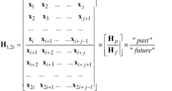
The null subspace (NSA) and enhanced-PCA method (EPCA) proposed in [1, 2] respectively are variant methods of the PCA method obtained by exploiting Hankel matrices of the dynamical system [5]. The data-driven block Hankel matrix is defined in Equation 3, where 2i is a user-defined number of row blocks, each block contains m rows (number of measurement sensors), j is the number of columns (practically j = N-2i+1). The Hankel matrix , consists of 2im rows and is split into two equal parts of i block rows, which represent past and future data respectively. Compared to the observation matrix X, the Hankel matrix is built using time-lagged vibration signals and not instantaneous representations of responses. This enables to take into account time correlations between measurements when current data depend on past data. Therefore, the objective pursued here in using block Hankel matrices rather than observation matrices is to improve the sensitivity of the detection method. 1 2 2 3 1 1 1 1,2 1 2 2 3 1 2 2 1 2 1 ... ... ... ... ... ... ... ... ... ... ... " " ... ... " " ... ... ... ... ... ... ... ... ... j j i i i j p i i i i j f i i i j i i i j past future + + + − + + + + + + + + + − ⎡ ⎤ ⎢ ⎥ ⎢ ⎥ ⎢ ⎥ ⎢ ⎥ ⎢ ⎥ ⎡ ⎤ ⎢ ⎥ = ≡⎢ ⎥≡ ⎢ ⎥ ⎢⎣ ⎥⎦ ⎢ ⎥ ⎢ ⎥ ⎢ ⎥ ⎢ ⎥ ⎢ ⎥ ⎣ ⎦ x x x x x x x x x x x x x x x x x x H H H (3)
where the subscripts of , denote the subscript of the first and last element of the first column in the block Hankel matrix.
3. DAMAGE DETECTION BASED ON THE CONCEPT OF SUBSPACE ANGLE
The principal components contained in matrix U span a subspace, which characterizes the dynamic state of the system. Without any damage or variation of environmental conditions, the characteristic subspace U remains unchanged. Any change in the dynamic behaviour caused by a modification of the system state modifies consequently its characteristic subspace. This change may be estimated using the definition of subspace angles [6]. As illustrated by a two-dimensional case in Figure 1, the concept of subspace angle can be seen as a tool to quantify existing spatial coherence between two data sets resulting from observations of a vibration system. In the figure, an active subspace is built from two principal components (column vectors) of matrix U.
Figure 1 - Angle θ formed by active subspaces according to the reference and current states, due to a dynamic change
4. DAMAGE DETECTION IN THE CHAMPANGSHIEHL BRIDGE 4.1. Description of the bridge
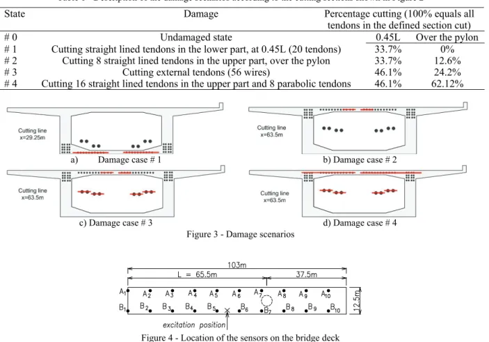
The Champangshiehl Bridge shown in Figure 2 is a two span concrete box girder bridge built in 1966 and located in the centre of Luxembourg. The bridge has a total length of 102 m divided into two spans of 37 m and 65 m respectively. It is pre-stressed by 112 steel wires as illustrated in Figure 2b. Before its complete destruction, the bridge was monitored and a series of damages were artificially introduced as summarized in Table 1. The four damage cases considered are illustrated in Figure 3a-d.
The measurement setup considered in the present work is given in Figure 4. Ten sensors were located on each side A and B of the deck (the distance between each sensor is about 10 m). Vibration monitoring under impact excitation was performed on the healthy structure and at each damage state. More detailed descriptions of the bridge can be found in [7].
a) Longitudinal section of the bridge
Figure 2 - The Champangshiehl Bridge
Table 1 - Description of the damage scenarios according to the cutting sections shown in Figure 2
State Damage Percentage cutting (100% equals all tendons in the defined section cut)
# 0 Undamaged state 0.45L Over the pylon
# 1 Cutting straight lined tendons in the lower part, at 0.45L (20 tendons) 33.7% 0% # 2 Cutting 8 straight lined tendons in the upper part, over the pylon 33.7% 12.6%
# 3 Cutting external tendons (56 wires) 46.1% 24.2%
# 4 Cutting 16 straight lined tendons in the upper part and 8 parabolic tendons 46.1% 62.12%
a) Damage case # 1 b) Damage case # 2
c) Damage case # 3 d) Damage case # 4 Figure 3 - Damage scenarios
Figure 4 - Location of the sensors on the bridge deck
4.2. Analysis results
The bridge may be analyzed through a well established modal identification method proposed in [8] which relies on the use of stochastic subspace identification (SSI). Two first eigenfrequencies obtained for the four damage cases (D1-D4) are compared to the eigenfrequencies of the healthy structure as reported in Table 2.
Table 2 shows that the decrease of the eigenfrequencies is proportional to the damage level for damage cases D1, D3 and D4. Only damage case D2 exhibits a different behaviour as the first eigenfrequency increases by an amount of 1.6 % with respect to the healthy case. Moreover, the second eigenfrequency is affected by the larger decrease (5.42 %) of all the damage states. This is in good agreement with an earlier analysis reported in [9]. The application of the concept of subspace angle on the Champangshiehl Bridge data allows to detect all the damage cases (D1-D4) using the single first principal component (PC) of the Hankel matrix. The detection remains good and even more evident when 2, 3 and 4 PCs are used.
On the other hand, the use of more PCs (higher than 4) deteriorates the quality of the distinction between the damaged and the healthy states. Indeed, the highest PCs (associated to small singular values i.e. low energy) come from noise present in the data and are not dynamic features of the system. As an example, the detection results obtained on the basis of 3 PCs is shown in Figure 5. In this figure, a total of 20 tests were considered: eight tests on the healthy structure (H) and twelve tests corresponding to the four levels of damages D1-D4. It
b) Schematic cross section of the box girder with location of the tendons
can be observed that all the damage cases are well detected and that damage cases D2 present the largest damage indexes.
Table 2 - Change in the eigenfrequencies (identified by SSI)
f1 f2 Value (Hz) Δf1 (%) Value (Hz) Δf2 (%) Healthy 1.92 5.54 D1 1.87 -2.6 5.45 -1.62 D2 1.95 1.6 5.24 -5.42 D3 1.82 -5.21 5.39 -2.71 D4 1.75 -8.85 5.3 -4.33
Figure 5 - Damage detection results using EPCA
5. DAMAGE DETECTION ON ECHOLUX PANELS 5.1. Description of the panels
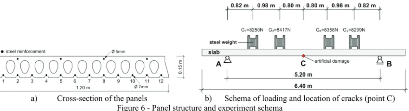
The two investigated panels are manufactured by the Luxembourg company ECHOLUX and both are of the same type (ECHOLUX-VSF-15-120, one prestressed concrete (PC), one special fabricated non-prestressed, reinforced concrete (RC) for testing purposes only). They are made of concrete C50/60 with an elastic modulus of 42700 N/mm2 and a measured compressive strength of 58.3N/mm2 (quality control of manufacturer). The quality of the reinforcement is St 1470/1670 and the corresponding elastic modulus 205000N/mm2. In the upper section of the panel, there are 4 wires with a diameter of 5mm and in the lower section 12 wires with a diameter of 7mm. Before testing, the concrete at the bottom side in the middle of the slab along axis C (Figure 6b) was removed, as shown in Figure 6a, to give access to the reinforcement for the later procedures of cutting tendons.
a) Cross-section of the panels b) Schema of loading and location of cracks (point C) Figure 6 - Panel structure and experiment schema
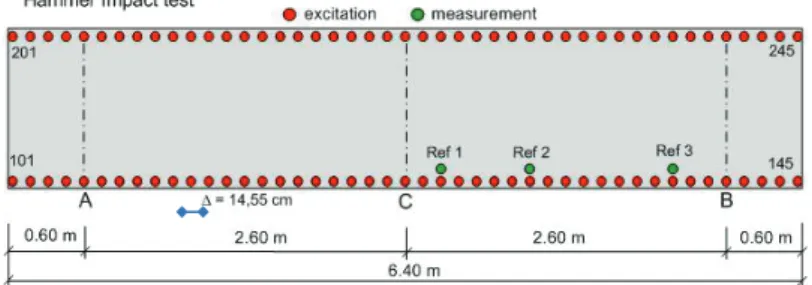
Both static and dynamic tests were performed on the slabs to compare their behavior in each condition [10]. The dynamic responses were measured using impact testing. The sample rate of the data acquisition is set to 200Hz; signals were recorded during 8 seconds after the introduction of impact. The measurements are set with a quite dense grid (∆=14.55 cm, Figure 7) for the sake of studying damage localization later. There are 45 impact points at each side of the slabs and three accelerometers (Ref 1-Ref 3 in Figure 7) are used to capture dynamic responses. So, in each condition, we have 3 sets of data containing 90 signals.
Damages were introduced by static mass loading (Figure 6b), cutting of steel wires and are resumed in Table 3. 5.2. Analysis results
Relating to frequency, damages show influence principally on the first component. Table 5 presents the first eigenfrequency shift, identified by the peak picking and SSI methods respectively.
The results obtained in Table 5 for the RC slab show a good agreement between the peak picking and SSI methods. It shows a clear decrease of frequency values following the increasing levels of damage. However, for the PC slab, the eigenfrequencies vary very slightly between different conditions, only the intact state (#0) and the state before the failure (#3*) are clearly distinct. The values identified by SSI cannot classify levels #0 to #2*. This is consistent with the observations and cracking described in Table 4: no change is noticed between state #0 to #1*. It reveals that in comparison with the RC slab, apparent damage occurs very late in the PC slab; the crack formation and hence the deformation is negligible until failure, which makes the detection more difficult.
Figure 7 - Measurement setup: impact point (101-145 and 201-245) and accelerometer positions (Ref 1 - Ref 3)
Table 3 - Damage scenarios
No. Damage scenario Cutting percentage Remark
#0 Intact state – no damage ‐ Later we consider states #0, #0*, #1*, #2*, #3*.
* denotes a state after loading and then removing of 4 heavy weights from the slab (shown in Figure 6b) #1 Cutting of 2 tendons (n0 6,7 - refer to Figure 6a) 16.7%
#2 Cutting of 4 tendons (n0 6, 7, 2, 11) 33.3% #3 Cutting of 6 tendons (n0 6, 7, 2, 11, 4, 9) 50% #4 Cutting of 8 tendons (n0 6, 7, 2, 11, 4, 9, 3, 10) 66.7%
Table 4 - Description of damages
No. Reinforced concrete (RC) slab Prestressed concrete (PC) slab
#0 No damage No damage
#0* Appearance of a decisive crack pattern, large creep No crack observed
#1* No further cracks, current cracks grow and also creep No crack observed, no considerable deformation #2* As above Appearance of a hairline crack , minimal deformation
#3* As above As above
#4* Collapse Collapse
Table 5 - The shift of the first eigenfrequency (Hz) from the intact state until before the collapse (always unloaded state)
RC slab PC slab
State #0 #0* #1* #2* #3* #0 #0* #1* #2* #3*
f by peak picking 11 9.18 8.07 7.85 7.69 11.75 11.70 11.65 11.65 11.55 f by SSI 11 9.20 8.00 7.70 7.60 11.73 11.65 11.61 11.56 11.33 Before the implementation of the static and dynamic tests, cracking loads were calculated for each structure. For the RC slab, the cracking load is expected for a load of two steel weights (G1 and G2 in Figure 6b) without cutting of any wires. Contrarily, the cracking load for the PC slab is expected for an additional load of four steel weights (G1, G2, G3 and G4) and cutting of 6 to 7 wires.
As presented in Figure 8, EPCA detects dynamic change in the RC slab from the loading of 2 masses, what corresponds already to the cracking load, while visible cracks are noticed only after the loading of 4 masses. Furthermore, the results distinguish clearly the tests before and after cutting tendons: larger subspace angles are obtained for the last cases. All signals processed here were measured after a procedure of charging then removing masses. Each condition is represented by 3 sets of measurement, one set of measurement in the intact state is provided for reference data.
For the PC slab, it is theoretically proven that the cracking load can be reached much later with respect to the RC slab. Only a hairline crack occurs after the loading of 4 masses in addition to the cutting of 4 tendons (#2*). In this circumstance, for a more precise comparison between different conditions in the PC slab, we examine only the correlation of states after a procedure of loading then removing the 4 masses. All data refer to the intact state #0* after the removing the masses. As presented in Figure 9, the EPCA method is able to detect well the
damages caused in the slab. As in the visible observations, subspace angles do not reveal much difference between damages #1* to #3*.
Figure 8 - EPCA detection for the RC slab (always unloaded state)
Figure 9 - EPCA detection for the PC slab (always unloaded state)
5.3. Localization of damage
5.3.1 Index for localization
In the previous sections, the SSI and EPCA methods were used in the time-domain for modal identification and damage detection.Damage may be located based on the estimation of flexibility from the identified mode-shapes as presented in [7]. In this section, Principal Component Analysis (PCA) is used for damage localization based on a sensitivity analysis in the frequency-domain. The technique is described in earlier works [2, 11, 12] and is summarized here briefly.
Let us consider the Frequency Response Functions (FRFs) Hs( )ω for a single input at location s:
( ) ( )
1 2( )
( ) ... s N ω = ⎣⎡ ω ω ω ⎤⎦ H h h h (4)where vector h
( )
ωk is of dimension m (the number of measured co-ordinates) and N is the number of frequency lines. The rows of Hsrepresent the responses at the measured degrees of freedom (DOFs), while the columns are “snapshots” of the FRFs at different frequencies. We will assume that the dynamical system matrices depend on a vector of parameters p. This vector of parameters may consist of system parameters or state variables. We can assess its principal components through Singular Value Decomposition (SVD) as represented in Equation (2). As Hsbelongs to the frequency-domain, the left singular vectors in give spatial information, the right singular vectors in represent modulation functions depending on frequency and the diagonal matrix of singular values contains scaling parameters of descending order σ1>σ2> >... σm. In other words, the SVD of HsFrom Equation (2), a sensitivity analysis can be performed by taking the derivative of the observation matrix with respect to p: T T T s ∂ =∂ + ∂ + ∂ ∂ ∂ ∂ ∂ H U Σ V ΣV U V UΣ p p p p (5)
Through this equation, the sensitivity of the system dynamic response shows its dependence on the sensitivity of each SVD term. Junkins and Kim [13] developed a method to compute the partial derivatives of SVD factors. Here for the sake of localization, we are more particularly interested in spatial information contained in the left singular vector U; its sensitivity with respect to a parameter pk is simply given by the following equation:
1 m k i ji j k j p =α ∂ = ∂
∑
U U with T T T 2 2 1 s s k ji i j i j i j k k i j p p α σ σ σ σ ⎡ ⎛ ∂ ⎞ ⎛ ∂ ⎞ ⎤ ⎢ ⎥ = ⎢ ⎜⎜ ⎟⎟+ ⎜⎜ ⎟⎟ ⎥ ∂ ∂ − ⎝ ⎠ ⎝ ⎠ ⎣ ⎦ H H U V U V (6)It is shown in [13] that the diagonal coefficients αiik keep only their imaginary part (their real parts are empty). So, the sensitivity of the ith principal component can be computed through coefficients αkji which depend on an unknown∂Hs/∂pk. It is proven in [11] that when the system matrices are symmetric, if parameter of interest is some coefficient ke of the stiffness matrix, the sensitivity of the FRF matrix may be simply determined by the
following formula: , / . e e s k k k s p ∂H ∂ = −H H (7)
where H is just the row vector corresponding to coefficient kke e in the FRF matrix in equation (4) and Hk se, is the s element of this vector.
Once ∂Hs/∂pk has been computed, the sensitivity of the left singular vectors is a good candidate for resolving localization problems of linear-form structures, e.g. chain-like or beam-like structures. In each working condition of the system, we can compute the sensitivity ∂Ui/∂pk . The reference state is denoted by ∂UiR/∂pk, and the deviation of the current condition may be assessed as follows:
R i i i k k k p p p ∂ ∂ ∂ Δ = − ∂ ∂ ∂ U U U (8) The last vector allows the maximization of useful information for damage localization.
5.3.2. Application on the ECHOLUX panels
First, let us note that the sensitivity analysis of the FRF data allows extracting structural mode-shapes thanks to the principal component vectors contained in matrix U. For the sake of conciseness, only the signals coming from one slab side are used here (from point 101 to 145 in Figure 7). Figure 10 compares the mode-shapes identified through SSI and the sensitivity analysis respectively. It clearly shows that the mode-shapes obtained by the sensitivity analysis are smoother than by SSI. The SSI modes show larger variations at points of high amplitude.
As stated before, damage produces a crack pattern in the middle of the slab. So it is expected that the damage localization procedure will point out damage around this zone, i.e. along axis C passing through point 23 (see Figure 7) which marks the middle of the slab.
Let us remind that in PCA, a large number of data is one of the requirements so that a principal component in U converges to a modal vector; so a frequency range should be chosen large enough for a sufficient observation of data in Hs( )ω . For the RC slab, the frequency range of [4 Hz – 26 Hz] corresponding to mode 1, is first selected to eliminate low-frequency noise and higher frequency modes.
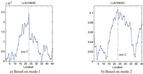
The results for 1 k p ∂ Δ ∂ U
shown in Figure 11 are obtained from the set of measurement n°3. As the sensor was located at point 38 for this set of measurement, parameter pk is chosen to correspond to k38 according to the 38th element of the ‘experimental’ stiffness matrix. The ‘undamaged’ vector of ∂U1/∂pk is extracted from state #0 which is considered as reference. The diagrams of 1
k p ∂ Δ ∂ U
in Figure 11 show for both mode 1 and 2 that the highest peaks are located close to point 23 (axe C) where the cracks gather. To take into account higher frequency component (mode 2), the frequency range of [4 Hz – 50 Hz] is considered and the results are given in Figure 11b. It should be noticed that the first principal component represents mode 2 of the structure, as shown
in Figure 10b. Mode 2 which is more dominant than mode 1, is also more sensitive to damage. If only mode 1 is used, damages are only detected in cases #2*, #3* but they are detected in all cases #0* - #3* when mode 2 is used. For the sake of conciseness, only the results for damage #2* are presented here as an example.
a) Mode-shapes obtained by SSI
b) Mode-shapes obtained by the sensitivity analysis
Figure 10 - Comparison of mode-shapes obtained by SSI and the sensitivity analysis (x: position of support)
a) Based on mode 1 b) Based on mode 2 Figure 11 - Damage localization in the RC slab for damage #2*
In the case of PC slab, damages are detected much later and less apparent than in the RC slab, just before its collapse. It is confirmed by very small changes in frequencies under different conditions.
The localization procedure does not give any interesting outcome for the PC slab when only mode 1 is considered. However, as in the RC slab, the use of mode 2 also allows a better localization. Damages #3* and #2* can be similarly localized as shown in Figure 12. The peak does not arise exactly at point 23 (along axis C) but in the neighboring area.
6. CONCLUSION
Several variants of Principal Component Analysis have been used in this study for detection and localization of damage. The advantage of PCA over classical modal identification methods relies on its easiness of use. The first results obtained on the Champangshiehl bridge are very encouraging. Furthermore, damage localization and the influence of environmental conditions on the diagnosis will be considered. The examples of the ECHOLUX panels showed that the damages were better distinguished on the basis of the first eigenfrequency (especially for the RC slab) while they were localized in a more effective manner using the second mode-shape.
ACKNOWLEDGMENT
The author Nguyen V. H. is supported by the National Research Fund, Luxembourg. 7. REFERENCES
[1] Yan A.-M., Golinval J.-C., “Null subspace-based damage detection of structures using vibration measurements”, Mechanical Systems and Signal Processing 20, 2006, pp. 611-626.
[2] Nguyen V.H., “Damage Detection and Fault Diagnosis in Mechanical Systems using Vibration Signals”, 2010, PhD dissertation, University of Liège.
[3] Nguyen V.H., Rutten C., Golinval J.-C., “Fault Diagnosis in Industrial Systems Based on Blind Source Separation Techniques Using One Single Vibration Sensor”, Shock & Vibration 5, 2012, pp. 795-801. [4] De Boe P., “Les éléments piézo-laminés appliqués à la dynamique des structures”, PhD dissertation,
2003, University of Liège.
[5] Overschee P. V., De Moor B., “Subspace identification for linear systems-Theory-Implementation-Applications”, Kluwer Academic Publishers, 1997.
[6] Golub G.H., Van Loan C.F., “Matrix computations”, Baltimore, The Johns Hopkins University Press, 1996.
[7] Mahowald J., Maas S., Waldmann D., Zürbes A., Scherbaum F., “Damage Identification and Localisation Using Changes in Modal Parameters for Civil Engineering Structures”, Proceedings of the International Conference on Noise and Vibration Engineering, 2012, Leuven, Belgium, pp. 1103–1117.
[8] Peeters B., De Roeck G., “Stochastic System Identification for Operational Modal Analysis: A Review”, Journal of Dynamic Systems, Measurement and Control, Transaction of the ASME, vol 123, 2001, pp. 659-667.
[9] Mahowald J., Maas S., Scherbaum F., Waldmann D., Zürbes A., “Dynamic damage identification using linear and nonlinear testing methods on a two-span prestressed concrete bridge”, Proceedings of the Third International Symposium on Life-Cycle Civil Engineering, Vienna, Austria: CRC Press, pp.157–164. [10] Mahowald J., Bungard V., Waldmann D., Maas S., Zürbes A., De Roeck G., “Comparison of linear and
nonlinear static and dynamic behaviour of prestressed and non-prestressed concrete slab elements”, Proceedings of The International Conference on Noise and Vibration Engineering 2010, Leuven, Belgium, pp. 717–728.
[11] Nguyen V.H., Golinval J.-C., “Damage localization in Linear-Form Structures Based on Sensitivity Investigation for Principal Component Analysis”, Journal of Sound and Vibration 329, 2010, pp. 4550-4566.
[12] Todd Griffith D., “Analytical sensitivities for Principal Components Analysis of Dynamical systems”, Proceedings of the IMAC-XXVII, Orlando, Florida, USA, February 9-12, 2009.
[13] Junkins J.L. and Kim Y., “Introduction to Dynamics and Control of Flexible Structures”, AIAA Education Series, Reston, VA, 1993.