Duclos: Département d’économique and CIRPÉE, Université Laval, Canada, and Institut d’Anàlisi Econòmica (CSIC), Spain
Makdissi: Department of Economics, University of Ottawa, P.O. Box 450, Station A, Ottawa, Ont., Canada K1N 6N5 and CIRPÉE
Araar: Département d’économique and CIRPÉE, Pavillon deSève, Université Laval, Québec, Canada G1V OA6
This work was carried out with support from SSHRC, FQRSC and the Poverty and Economic Policy Research Network, which is financed by the Government of Canada through the International Development Research Centre and the Canadian International Development Agency, and by the Australian Agency for International Development. We are grateful to Sami Bibi for useful comments and to Lourdes Trevio and Jorge Valero Gil for having facilitated
Cahier de recherche/Working Paper 10-01
Pro-Poor Tax Reforms, with an Application to Mexico
Jean-Yves Duclos Paul Makdissi Abdelkrim Araar
Abstract:
This paper proposes a methodology for testing for whether tax reforms are pro-poor. This is done by extending stochastic dominance techniques to help identify tax reforms that will necessarily be deemed absolutely or relatively pro-poor by a wide spectrum of poverty analysts. The statistical properties of the various estimators are also derived in order to make the method implementable using survey data. The methodology is used to assess the pro-poorness of possible reforms to Mexico’s indirect tax system. This leads to the identification of several possible pro-poor tax reforms in that country. It also shows how the pro-poorness of a tax reform depends on one’s conception of poverty as well as on the revenue and efficiency impact of the reform.
Keywords: Stochastic dominance, pro-poor changes, tax reforms, Mexico
1 Introduction
Recent policy objectives have often focused on improvements in the well-being of the less fortunate in society. There are several reasons for this: some are related to a rise in the ethical and policy importance of poverty reduction (best exemplified by the salience of the United Nations’ Millenium Development Goals), while others are linked to more specific conditions, such as concerns for the effect on the poor of food price variability and of the recent global financial and economic crisis.
Signs of such policy interest abound, regarding particularly the use of indirect taxation and subsidies as tools for poverty alleviation. For instance, a report from an initiative recently launched by the UNDP, the Government of China and DFID states that “the depth and coverage of China’s fiscal reform process has been un-even, and there is scope for strengthening the links between fiscal reforms and poverty reduction goals.”1 Commentators in the Philippines have argued that the “fiscal crisis hurts the poor Filipinos more than it hurts the rich and the big cor-porations. [...] Only under a pro-poor management of the fiscal crisis will make Filipinos rally behind the Arroyo administration during this difficult time.”2 One element of the reaction of the Filipino government has indeed been to expand the use of the Value Added Tax (VAT) because it claims that “its burden falls heavier on those who consume more ’VATable’ goods and services.”3
In India, the press has “wanted Finance minister P. Chidambaram to balance tight fiscal policy with pro-poor policies”.4 The recent 2008 Pakistan budget has also been criticized because it “was hoped that the current government would realise that achieving fiscal discipline and increasing revenues is important, but not on the backs of the poor. If the government wants to address the challenges of inflation, rising inequality and poverty, it must devise a progressive taxation policy that relies less on indirect taxes and more on increasing the tax-GDP ratio by extending the tax net to untaxed sectors.”5 Concerns for the poverty effect of government financing procedures have also extended to other areas, such as how health care financing systems can be designed and implemented to be ’pro-poor’ (see for instance Bennett and Gilson 2001). This naturally suggests the broader
1http://www.undp.org.cn/projects/39815.pdf. 2http://aupwu.blogspot.com/2004/11/pro-poor-response-to-fiscal-crisis.html. 3http://www.sunstar.com.ph/static/dav/2006/02/13/bus/expanded.vat.is.pro.poor.solon.html. 4 http://www.financialexpress.com/news/fm-should-balance-policy-with-propoor-plans-fitch/127916/. 5http://www.opfblog.com/2901/is-pakistan-budget-2008-pro-poor-by-sadia-m-malik/.
policy problem of using a tax and expenditure system to minimize poverty subject to some government budget constraint. As is well-known, an overriding tradeoff in such problems is to balance potential gains in equity and in efficiency.
The last decade has also seen several conceptual and empirical contributions on whether growth is “pro-poor”. A central issue is whether the poor’s benefits from growth exceed some norm — see, among many recent interesting contribu-tions to that issue, Bruno, Ravallion, and Squire (1998), United Nacontribu-tions (2000), Eastwood and Lipton (2001), Ravallion (2001), Dollar and Kraay (2002), World Bank (2002) and Bourguignon (2003). This norm may be absolute or relative to the changes in the entire distribution of income, as discussed for example in Duclos (2009).
A similar issue applies to the effect of public policy in general. As is clear from the above, we may wish for instance to assess whether a fiscal reform is “pro-poor”, in the sense that the benefits that the poor derive from it exceed some norm. Unfortunately, as with many other distributive assessments, the precise definition that can be given to the pro-poorness of a tax reform is essentially a matter of normative judgement and can be open to the criticism of being arbitrary to at least some extent. Elements of arbitrariness arise inter alia in the choice of a poverty line to separate the poor from the non-poor and in the choice of an aggregative procedure to summarize the reform’s impact on the poor.6 To show how one can reduce these sources of arbitrariness in understanding pro-poorness is the first main objective of this paper.
The second main objective of the paper is to assess how and whether a (margi-nal) tax reform can be considered to be pro-poor. Santoro (2007) categorizes the economic literature on the impact of marginal tax reforms into three different approaches. The first is based on Ahmad and Stern (1984) and uses a specific social welfare function. The second identifies directions for marginal tax reforms based on classes of social welfare functions that display an aversion to inequal-ity and that are symmetric — this was introduced by Yitzhaki and Thirsk (1990), Yitzhaki and Slemrod (1991) and Mayshar and Yitzhaki (1996). The third ap-proach supposes that marginal tax reforms can also be used as instruments for changing poverty and is based inter alia on Makdissi and Wodon (2002), Duclos, Makdissi, and Wodon (2008) and Liberati (2003).
This paper extends this third approach by testing for whether indirect tax
re-6Different approaches have been proposed to separate the poor from the non-poor and to com-pute indices of “growth pro-poorness”. See, for instance, McCulloch and Baulch (1999), Ravallion and Datt (2002), Kakwani, Khandker, and Son (2003), Ravallion and Chen (2003), Klasen (2004), Son (2004), Essama-Nssah (2005), and Araar, Duclos, Audet, and Makdissi (2007).
forms can be considered to be pro-poor. By this, it is meant that an indirect tax reform must be deemed to be “equitable towards the poor” or “in favor of the poor”, in the sense that the benefits of the reform must accrue (in some sense to be made precise later) “more” to the poor, or that its costs must hurt “less” the poor.
The first and second main objectives are dealt with in Section 2. The results are general enough to cover the cases of negative (subsidies) and positive indirect taxation, and of tax reforms that may or may not be revenue and/or efficiency neutral. Although for expositional simplicity the paper focusses on indirect tax changes, the methodology can be relatively easily adapted to deal with the effect of changes in direct taxation and in-kind benefits. Section 2 further hints to how the paper’s framework and analytical results can also be used to assess the impact of tax reforms on absolute and relative inequality.
The analytical results of Section 2 show that whether tax reforms involving only one good are pro-poor depend roughly on whether the good is an inferior, a necessary, or a luxury one. More generally, the pro-poorness of a tax reform depends on a mixture of income (for redistribution) and price (for efficiency) elas-ticities that are easily combined to check for necessary and sufficient conditions for whether the tax reform can be considered to be unambiguously pro-poor. Al-though simple to test for, the pro-poorness of a tax reform can nevertheless differ quite significantly from the optimal taxation literature’s results on whether a tax reform improves social welfare.
For instance, an efficiency-neutral and revenue-neutral tax reform that in-creases the price of good j but dein-creases the price of good i is absolutely and relatively pro-poor if the poor’s (weighted) share of the total consumption of good
i exceeds their (weighted) share of the total consumption of good j, the shares
being given by the poor’s poverty gaps. If, however, real income falls after the tax reform (because of a rise in the total deadweight loss), relative pro-poorness demands that the share of the poor in total real income does not fall after the re-form, but absolute pro-poorness demands that the absolute real income of the poor does not fall after the reform by more than the absolute fall in total real income. An economically inefficient reform will therefore be more likely to be absolutely pro-poor than relatively pro-poor.
The more inefficient it is to tax a good, the greater the tax rate that must be levied on that good to generate the tax revenues needed to decrease taxes on an-other, less price-elastic, good. If the more price-elastic good is not a luxury good, this makes increasing its price less likely to be relatively pro-poor. Only when the price-elastic good is also a luxury good will an increase in its tax be conducive to greater relative pro-poorness. An efficiency-decreasing tax reform will also be
more likely to be considered relatively pro-poor than absolutely pro-poor as the importance given to the poorest of the poor increases.
Section 3 then proceeds by proposing estimators and deriving sampling dis-tributions for the tools needed to test for tax pro-poorness. This is needed to implement the analytical methods using survey data. For the important case of first-order pro-poorness, these estimators involve non-parametric regressions, for which the sampling distributions that need to be derived are more involved. The estimators and their sampling distributions cover all of the possible analytical cases derived in Section 2.
Section 4 applies the methodology to Mexico’s indirect tax system using Mex-ico’s 2004 ENIGH database. We find for instance that a marginal tax reduction on
Food or on Energy would be relatively pro-poor, and that this conclusion would be
valid for a very large class of relative pro-poor judgements. But, according to the paper’s definition of absolute pro-poorness, a marginal reduction in taxes on any of the different goods considered would need to be thought of as being absolutely
anti-poor. A revenue- and efficiency-neutral tax reform that decreases Food taxes
and increases Transportation taxes would be considered absolutely and relatively pro-poor for all indices and lines within a wide class and range. The application also shows that applying statistical inference techniques can alter conclusions in a way that sometimes contrasts importantly with the analysis made solely on the basis of sample estimates.
Section 5 concludes by summarizing briefly the main results. Most of the proofs of the main results can be found in the Appendix of Section 6.
2 Notation and methodological framework
2.1 Poverty Measurement
We first start with the presentation of rather general views of how poverty and tax pro-poorness can be assessed. For simplicity, suppose that poverty indices are additive7 and therefore take the form of
P (z) =
Z ω 0
p (y, z) dF (y) , (1)
7The Foster, Greer, and Thorbecke (1984) indices are an example of popular additive poverty measures. Other examples of additive indices can be found in Watts (1968), Clark, Hemming, and Ulph (1981) and Chakravarty (1983).
where y is real income, z is the poverty line (in real terms), F (·) is the cumulative distribution function of income with support over [0, ω], and p (y, z) is a function that measures the poverty of an individual with an income y and using a poverty line z. We suppose that p (y, z) ≥ 0 and that p (y, z) = 0 for all y > z. Duclos and Makdissi (2004) use the properties of P (z) to define classes of poverty indices Πs(z) for some order s. These classes are defined by:
Πs(z) = P (z) ¯ ¯ ¯ ¯ ¯ ¯ p(y, z) ∈ bCs(z),
(−1)ip(i)(y, z) ≥ 0 for i = 0, 1, 2, ..., s,
p(t)(z, z) = 0 for t = 0, 1, 2, ..., s,
(2)
where p(i)(y, z) represents the i-th derivative of p (y, z) with respect to y and bCs
is the set of continuous functions that are s-times differentiable on [0, ω].
For poverty indices P ∈ Π1(z), an increase in the income of any one individ-ual will weakly reduce the poverty index. This class of indices is thus Paretian. The indices are also symmetrical since exchanging incomes between two individ-uals will not affect poverty (by the property of the anonymous distribution func-tion in (1)). This type of indices can thus be said to satisfy Pen (1971)’s principles for comparing distributions (see Duclos, Makdissi, and Wodon (2008)).
The poverty indices included in Π2(z) are also convex. This implies that they respect the Pigou-Dalton principle of transfer, a principle that states that a transfer from any one individual to a poorer individual should weakly decrease poverty. In addition to obeying the above principles, the poverty indices that belong to Π3(z) must also obey the Kolm (1976) principle of transfers, which states that a Pigou-Dalton transfer that takes place at the bottom of the distribution should have a greater impact on poverty than one taking place higher up in the distribution. Hence, a progressive transfer that occurs within a lower part of the distribution will reduce poverty even if it is accompanied by a symmetric regressive transfer higher up in the distribution. Indices of a class Πs(z) with s greater then 3 can be
interpreted by using the generalized transfer principle proposed by Fishburn and Willig (1984). This generalized principle states that the greater the order s, the greater is the sensibility of an index to changes occurring in a lower part of the distribution.
2.2 Impact of price changes
Let us now suppose that we wish to test whether an indirect tax reform can be considered to be pro-poor. We consider three possible scenarios through which
this can be done.
1. The government wishes to implement a marginal reduction in the tax (or a marginal increase in the subsidy) on good i, without attempting to offset the fall in total government revenue (possibly because the government is running a budget surplus).
2. The government wishes to implement a marginal increase in the tax (or a marginal decrease in the subsidy) on good i, without attempting to offset the increase in total government revenue (possibly because the government is running a budget deficit).
3. The government wishes to implement a revenue-neutral indirect tax reform. It must therefore finance a marginal tax reduction on good i (or a marginal increase in its subsidy) with a marginal increase in the tax (or a marginal decrease in the subsidy) on good j 6= i.
Now assume that producer prices are held constant and, for expositional sim-plicity, set them to 1 so that q = e+t, where q is the vector of current consumption prices, e is a vector of ones, and t is the vector of indirect taxes. The impact of a marginal change dti to the tax on a good i will impact the poverty level of an
individual with income y by
∂p (y, z) ∂ti
= p(1)(y, z) ∂y
∂ti
. (3)
Using Roy’s identity and setting the vector of reference prices to the current price vector, the change in real income produced by a marginal change in the tax on good i is given by (see for instance Besley and Kanbur 1988)
∂y ∂ti
= −xi(y, q) , (4)
where xi(y, q) is the Marshallian demand of good i at the vector of current prices,
q. Introducing (4) into (3), we have that ∂p (y, z)
∂ti
2.3 Pro-poorness
We do not wish, however, to determine if a tax reform reduces or increases poverty, but rather if it can be considered pro-poor. This requires distinguishing between relative and absolute pro-poorness. We will say that a tax reform is R-pro-poor for relative R-pro-poorness and A-R-pro-poor for absolute R-pro-poorness. In the growth terminology of Duclos (2009) and Araar, Duclos, Audet, and Makdissi (2007), relative pro-poorness is checked by comparing P (z) using F1((1 + g)y) for a posterior distribution F1(y) to P (z) using an initial distribution F0(y), using a relative “norm” g (to be discussed later). Absolute pro-poorness with an absolute norm a (also discussed below) is checked by comparing P (z) using F1(y+a) for a posterior distribution F1(y) to P (z) using an initial distribution F0(y). Formally:
Definition 1 A movement from an initial distribution F0 to a posterior
distribu-tion F1 is judged relatively pro-poor by an index P (z) if and only if Z ∞ 0 p (y, z) dF1((1 + g)y) − Z ∞ 0 p (y, z) dF0(y) < 0. (6)
Definition 2 A movement from an initial distribution F0 to a posterior
distribu-tion F1 is judged absolutely pro-poor by an index P (z) if and only if Z ∞ 0 p (y, z) dF1(y + a) − Z ∞ 0 p (y, z) dF0(y) < 0. (7)
For expositional simplicity, we will assume for the purposes of this paper that the relative norm g is set to the growth rate of average real income. This is consis-tent with the view of Kakwani and Pernia (2000) (p.3) that “promoting pro-poor growth requires a strategy that is deliberately biased in favor of the poor so that the poor benefit proportionately more than the rich.” It is also consistent with the view that relative pro-poorness is tightly linked to inclusiveness and participation of the poor in growth processes and (more generally) in distributional changes. Setting g to the growth rate of average real income also allows linking relative pro-poorness to relative inequality reduction, as we will discuss more explicitly later.
Again for expositional simplicity, the absolute norm a is set in this paper to the numerical (as distinct from the proportional) change in average real income. Loosely speaking, this implicitly supposes that we wish distances between in-comes and the mean not to be increased by distributional changes. This also implicitly links absolute pro-poorness to absolute inequality reduction. Along
that view, a tax reform that decreases mean income because it increases govern-ment revenue could still be considered absolutely pro-poor, possibly because the increase in government revenue would allocate to everyone an increase in the ab-solute value of public goods equal to the increase in average government revenue. Generalizations of this to other settings would not be difficult, by setting for in-stance g to growth in some quantiles (such as the median), or by setting a to 0 (which would be equivalent to arguing that a change is pro-poor if it increases the poor’s absolute living standards — e.g., Ravallion and Chen 2003).
2.4 The impact of single price changes
Let then: y∗R = y 1 + g, (8) y∗A = y − a, (9) ∂p∗η(y, z) ∂ti = p(1)(y, z)∂y ∗η ∂ti , η ∈ {A, R}. (10)
We now wish to determine how y∗Rand y∗Avary with a marginal variation in
ti. The average impact of dtion real income in the total population is given by dti
times the average consumption of good i, which is denoted as Xi(q):
Xi(q) =
Z ∞ 0
xi(y, q) dF (y) . (11)
Using this, the proportional change in average real income (following a change
dtiin a tax rate ti) is given by
−Xi(q)
µ dti, (12)
where µ = R ydF (y) is average income. The absolute change in average real
income is given by
−Xi(q) dti. (13)
In order to determine the impact of a marginal variation in ti on y∗Rand y∗A,
real income of the change in the pro-poor norm given by (8) and (9). This leads to ∂y∗R ∂ti = −xi(y, q) + y Xi(q) µ (14) and ∂y∗A ∂ti = −xi(y, q) + Xi(q). (15)
Using (14) and (15), we obtain
∂p∗R(y, z) ∂ti = −p(1)(y, z) · xi(y, q) − y Xi(q) µ ¸ (16) and ∂p∗A(y, z) ∂ti = −p(1)(y, z) [x i(y, q) − Xi(q)] . (17)
To obtain the impact on total poverty, we integrate (16) and (17) over the entire income distribution. The result is
∂P∗R(z) ∂ti = − Z ∞ 0 p(1)(y, z) · xi(y, q) − y Xi(q) µ ¸ dF (y) (18) and ∂P∗A(z) ∂ti = − Z ∞ 0
p(1)(y, z) [xi(y, q) − Xi(q)] dF (y) . (19)
2.5 Testing for pro-poorness of single price changes
We can now introduce pro-poor consumption dominance curves (CDη:s), η ∈
{A, R} and s ∈ {1, 2, 3...}.8 Those pro-poor consumption dominance curves are defined as: CDR:si (z) = h xi(z,q) Xi(q) − z µ i f (y) for s = 1 z R 0 CDR:s−1i (y) dy for s ≥ 2, (20)
and CDA:si (z) = h xi(z,q) Xi(q) − 1 i f (z) for s = 1, z R 0
CDA:s−1i (y) dy for s ≥ 2. (21) By integration by parts, (20) and (21) can be written for s = 2, 3, ... as
CDR:s i (z) = 1 (s − 2)! z Z 0 · xi(y, q) Xi(q) − y µ ¸ (z − y)s−2dF (y) (22) and CDA:si (z) = 1 (s − 2)! z Z 0 · xi(y, q) Xi(q) − 1 ¸ (z − y)s−2dF (y). (23) This leads to our first main analytical result.
Theorem 1 A marginal decrease in the tax on good i is η-pro-poor (η ∈ {A, R}) for all indices P (z) ∈ Πs(z) and for all poverty lines z ∈ [0, z+] if and only if
CDη:si (z) ≥ 0, ∀z ∈£0, z+¤. (24) It is useful to interpret Theorem 1 in the context of the first two scenarios listed at the beginning of Section 2.2 on page 6. For this, let us first classify goods according to their income elasticity, εyi.
Definition 3 A good i is said to be an inferior good if εyi < 0 and a normal good if εyi > 0, for all y.
Definition 4 A normal good is said to be a necessary good if εyi < 1 and a luxury good if εyi > 1, for all y.
Four simple remarks can then be made as a corollary to Theorem 1.
Corollary 1 Regardless of the value of s and z+:
1. a reduction (an increase) in the tax of good i is never (always) A-pro-poor if the good is a normal good;
2. a reduction (an increase) in the tax of good i is always (never) A-pro-poor if the good is an inferior good;
3. a reduction (an increase) in the tax of good i is never (always) R-pro-poor if the good is a luxury good;
4. a reduction (an increase) in the tax of good i is always (never) R-pro-poor if the good is a necessity.
The income elasticities εyi do not of course have to be uniformly negative, positive, or below or above 1 for all values of y. When elasticities are not so uniformly distributed, condition (24) will have to be checked on a case-by-case distributional basis using Theorem 1.
2.6 Testing for pro-poorness of tax reforms
The above results are useful only in the cases in which only one tax or one price is changed, if for instance the government does not necessarily want to keep its overall revenue unchanged. For the case of a revenue-neutral tax reform sce-nario, one must finance a marginal tax reduction for a good i by a marginal in-crease in the tax on a good j in order to keep overall tax revenue constant. To show how to do this, suppose that there are K consumption goods and denote by
R the per capita tax revenue of the overall indirect tax system: R(q) =
K
X
k=1
tkXk(q). (25)
The impact of the marginal tax reform on per capita tax revenue is then given by
dR: dR = " Xi(q) + K X k=1 tk∂Xk(q) ∂ti # dti+ " Xj(q) + K X k=1 tk∂Xk(q) ∂tj # dtj. (26)
Revenue neutrality implies that dR = 0. Using (26), this leads to:
dtj = −γ µ Xi(q) Xj(q) ¶ dti where γ = 1 + 1 Xi(q) PK k=1tk ∂Xk(q) ∂ti 1 + 1 Xj(q) PK k=1tk∂X∂tkj(q) . (27)
Wildasin (1984) describes γ as the efficiency cost ratio of obtaining one dollar of public funds by taxing good j to subsidize good i. We can now state our second main result.
Theorem 2 A marginal tax reduction on good i financed by a marginal increase in the tax on good j is η-pro-poor (η ∈ {A, R}) for all indices P (z) ∈ Πs(z) and
for all poverty lines z ∈ [0, z+] if and only if
CDη:si (z) − γCDη:sj (z) ≥ 0, ∀z ∈£0, z+¤. (28) The proof follows directly from that of Theorem 1.
2.7 Discussion
Yitzhaki and Thirsk (1990) and Yitzhaki and Slemrod (1991) find that if γ is superior to one, it is impossible to secure a second-order welfare dominant tax reform due to the efficiency loss incurred. From a poverty perspective, Makdissi and Wodon (2002) note, however, that it is possible to have a reform that is domi-nant at all orders of stochastic dominance even when γ is greater than one, so long as that part of the burden is supported by the non poor.
This is also true here in the context of R and A pro-poorness. In (28), it is the weighted difference between CDη:si (y) − γCDη:sj (y) that matters. A tax reform can be economically inefficient (with γ > 1) and still be considered to be pro-poor if CDη:sj (y) is not too large.
Theorems 1 and 2 can also be used to assess the impact of price changes and tax reforms on absolute and relative inequality for any given order of dominance. This is because of the specification of a and g chosen in this paper. In (8) for relative pro-poorness, post-reform incomes are normalized by the ratio of aver-age real incomes. This essentially serves to equalize averaver-age real incomes across the pre- and the post-reform distributions. Using Duclos and Makdissi 2004, the conditions (2) on the class of evaluation functions then make it possible to use Theorems 1 and 2 to provide unambiguous conclusions on the impact of price changes and tax reforms on relative inequality.
For absolute pro-poorness, (9) essentially centers real incomes around their respective mean value. That makes it possible to use Theorems 1 and 2 to provide unambiguous conclusions on the impact of price changes and tax reforms on ab-solute inequality — that is, on inequality indices that aggregate distances between
incomes and their mean value in a way that is consistent with the conditions de-fined in (2).
When s = 1 and when γ = 1 (when there is no efficiency benefit or cost to the tax reform), Theorem 2 says that a tax reform is absolutely pro-poor if the poor’s share of the total consumption of good i exceeds their share of the total consumption of good j. Exactly the same interpretation applies to the relative pro-poorness of a tax reform when γ = 1: the poor’s share of the total consumption of good i must exceed their share of the total consumption of good j. This is because mean real income is unaffected by a revenue-neutral tax reform when γ = 1.9
When γ 6= 1, the interpretation of A and R pro-poorness differs. Take γ > 1, a case in which average real income falls after the tax reform (because of the efficiency cost). This is analogous to a case of negative growth. Relative pro-poorness demands that the share of the poor in total real income does not fall after the reform. Absolute pro-poorness demands that the absolute real income of the poor does not fall after the reform by more than the absolute fall in total real income. Since the initial share of the poor in total income is less than one (y/µ is less than one in (22)), an economically inefficient reform will be more likely to be absolutely pro-poor than relatively pro-poor.
The reverse reasoning applies to the case of an economically efficient tax re-form, for which γ < 1 and average real income increases. Relative pro-poorness demands that the share of the poor in total real income increases after the reform, and absolute pro-poorness will require that the absolute real income of the poor increases by more than total real income after the reform. Because of this, an economically efficient reform will be more likely to be relatively pro-poor than absolutely pro-poor.
If γ < 1, a reform will also be more likely to be considered relatively pro-poor than absolutely pro-pro-poor as s increases. The converse holds if γ > 1. This is because the greater the value of s, the greater the importance given to the poor-est of the poor in assessing pro-poorness conditions. (20) and (21) show that the standard in assessing relative pro-poorness is the difference between shares in the consumption of a good and shares in total income, but that the standard in assess-ing absolute pro-poorness is the difference between shares in the consumption of a good and 1. For the poor, that difference for relative pro-poorness will be larger than for absolute pro-poorness. Since an increase in s increases the importance given to the poorer individuals, ceteris paribus, an increase in s will also lead more quickly to the validation of (28) for η = R than for η = A if γ < 1, and
9When γ = 1, we have g = a = 0 since X
more quickly to the validation of (28) for η = A than for η = R if γ > 1. If γ = 1 this difference vanishes as the conditions for relative or absolute pro-poorness of tax reforms become both equivalent to the condition that a tax reform reduces poverty (see Duclos, Makdissi, and Wodon 2008).
3 Estimation and inference
To be able to implement empirically the above tools, we ought to consider the estimation and the sampling distribution of the curves needed to test for pro-poorness. For this, we suppose for expositional simplicity that we dispose of a sample of N independently and identically distributed observations,10 and that the pre-reform income and consumption of goods j and l for observation i (i = 1, ..., N ) are denoted by yi, xij and xil, respectively. Ignoring the constant (s−2)!1 , the CDη:s curves can then be estimated for s ≥ 2 by the natural estimators
d CDR:sk (z) = 1 N N P i=1 xi k(z − yi)s−2+ b Xk − 1 N N P i=1 yi(z − yi)s−2+ b µ (29) and d CDA:sk (z) = 1 N N P i=1 xi k(z − yi)s−2+ b Xk − 1 N N X i=1 (z − yi)s−2+ , (30) where f+ = max(0, f ), bXk = N1 PN
i=1xikis an estimator of average consumption
of good k, and bµ = 1
N
PN
i=1yiis an estimator of average income.
The estimators dCDη:sl (z)−γdCDη:sj (z) are given analogously. Let CDs(xk; z) =
Rz 0 xk(y, q) (z − y) s−2dF (y) and dCDs(x k; z) = N1 N P i=1 xi k(z − yi)s−2+ . The asymp-totic sampling distribution of dCDs(xk; z) for s ≥ 2 is given in Theorem 3.
Theorem 3 Let the second population moment of xk(y, θ) (z − y)s−2+ be finite.
Then, for s ≥ 2, N0.5³CDds(x
k; z) − CDs(xk; z)
´
is asymptotically normal with 10The analytical results can be extended to account for complex multi-stage sampling designs. Taking into sampling design is indeed done in the Mexican illustration below, using analytical asymptotic methods along the lines of those described in Duclos and Araar (2006), Chapter 16. More details can be obtained from the authors upon request.
mean zero and with asymptotic variance given by: lim N →∞N · var ³ d CDs(xk; z) − CDs(xk; z) ´ = (s − 2)!−2 Z ¡ xk(y)(z − y)s−2+ ¢2 dF (y) − CDs(x k; z)2. (31)
Prof: See the appendix.
The asymptotic distribution of dCDR:sk (z) and dCDA:sk (z) can be obtained by noting that (29) and (30) are functions of dCDs(xk; z), bXk, dCD
s
(y; z), bµ, and
d
CDs(1; z). The sampling distribution dCDs(y; z) and dCDs(1; z) can be obtained as special cases of Theorem 3. bµ and bXk are simple sums of independently and
identically distributed random variables. Using the “delta method” of Rao (1973), the sampling distribution of dCDA:sk (z) and dCDR:sk (z) can then be obtained by a linear transformation of the covariance matrix of dCDs(xk; z), bXk, dCD
s
(y; z), bµ,
and dCDs(1; z).
For s = 1, we need an estimator of xk(z, q), the expected consumption of
good k at z, times f (z). For this, we can use a non-parametric estimation proce-dure, using for instance a kernel estimator defined such as
d CD1(xk; z) = 1 N N X i=1 κh(z − yi) xik, (32)
where h is a kernel bandwidth, κh(u) = h−1κ (u/h),
R
κ(u)du = 1,R uκ (u) du =
0 (for symmetry), andR u2κ (u) du = c
κ. In the illustration below, we choose a
Gaussian form for κ (u),
κ (u) = e
−0.5u2 √
2π , (33)
but other kernel functional forms could also be used. In the illustration, we choose
h using the cross-validation method, which is asymptotically optimal (see H¨ardle
1990, Theorem 5.1.1) and we also a locally linear estimator to avoid biases at the lower bound of expenditures. Theorem 4 then gives the asymptotic sampling distribution of dCD1(xk; z).
Theorem 4 Let i)R κ (u)2du exists, ii) h ∼ N−0.2, iii) CD1
k(y) be twice
differ-entiable in y at y = z, iv) f (z) > 0, and v) ck(z) = xk(z)2 be continuous at z.
Then, (Nh)0.5³CDd1(xk; z) − CD1(xk; z) − h2Bk(z)
´
with mean 0 and limiting variance Vk(z), where Bk(z) = 0.5 cκ∂2CD1(xk; z)/(∂z)2
and Vk(z) = f (z)ck(z)
R
κ (u)2du.
Prof: See the appendix.
The sampling distribution of dCDR:1k (z) and dCDA:1k (z) can then be obtained by a linear transformation of the covariance matrix of dCD1(xk; z), bXk and bµ
using the delta method. As for s ≥ 2, the terms needed to carry out statis-tical inference are either constants (cκ and
R
κ (u)2du) or can be readily
esti-mated consistently in a distribution-free manner (this is the case, for instance, ofR ¡xk(z − y)s−2+
¢2
dF (y), dCDs(xk; z)2, ∂2CD1(xk; z)/(∂z)2, f (z) and ck(z)).
Note, however, that it is usual to consider (and to find) the bias terms Bk(z) and
Bk(z)/Xk to be of negligible practical importance11, and we also make this
as-sumption in the illustration below.
4 An application to Mexico’s indirect tax system
4.1 Mexican data
We now briefly apply the above methodology to Mexico’s indirect tax system. The data used for our application comes from the National Income and Expendi-ture (ENIGH) Survey collected in 2004, which is nationally representative of the Mexican population. ENIGH surveys collect information on incomes and expen-ditures, goods and services used for self-consumption, as well as socio-economic characteristics and labor market activities of all household members.
As is common in Latin America, we use total income per capita as the measure of living standards for all members of a household. To correct for spatial variation in prices, we assess all incomes in reference to rural prices and multiply urban household incomes by the ratio of rural to urban poverty lines. We use as a guide a 2004 rural poverty line set to 550 pesos per month per capita. To simplify the interpretation of figures and the discussion, we normalize income by that rural poverty line so that a household with an income equal to one is at the level of the rural poverty line and a household with an income of 2 has a real income equal to twice that line. We weight households by the product of household size and
11This is particularly true in the study of consumption data, where the second order derivative of expected consumption at z, ∂2CD1(x
k; z)/(∂z)2, may be expected to be small. For more on
household sampling weight; this is equivalent to formulating our estimators on the basis of the population of individual living standards.
We consider indirect tax reforms affecting four broad classes of goods and services (food, energy, transport and other goods) as well as various foodstuffs.12 Table 1 presents the percentage of total expenditure allocated to goods and ser-vices by quintile. As expected, the share of total expenditures on food items decreases from the poorest to the richest quintile. Conversely, the share of to-tal expenditures on transportation and other goods increases with quintiles. Table 1 also shows that the composition of the food basket varies with income quintiles; households in the poorest income quintile spend a greater share of their total food expenditure on cereals (25.88%) and on vegetables (19.30%) than those in the richest quintile — who spend relatively more (46.44%) on protein-intensive foods (milk, meat and fish).
4.2 Impact of tax changes
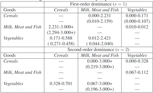
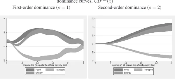
Figure 1 presents relative dominance curves CDR:s(z) for three broad classes
of goods and services and for s = 1, 2, along with two-sided 90% confidence in-tervals. Using the results of Theorem 1, this shows that a marginal tax reduction on
Food or on Energy would be relatively pro-poor, and that this conclusion would be
valid for any relative pro-poor judgements based on indices P ∈ Π1(z) (namely, those that in agreement with the Pen principle) for a wide range of poverty lines reaching almost 3. For s = 2, this is true for all possible poverty lines. Con-versely, a marginal increase in the tax on any of these two classes of goods would be considered relatively “anti-poor”. This suggests that it is important to consider the use to which increases in tax revenues are put to know whether a tax reform is globally pro-poor or not. We return to this below.
Figure 2 presents the corresponding absolute dominance curves CDA:s(z) for three broad classes of goods and services. A marginal reduction in taxes on any of the different goods could not be considered to be absolutely pro-poor. As in-dicated in Corollary 1, this result is not surprising considering the fact that the absolute pro-poor requirements are typically more demanding (since most goods are normal goods) than the relative ones (since not all normal goods are luxury goods) in the case of tax decreases. Conversely, increases in taxes on any of the different goods will be absolutely pro-poor for all P ∈ Π1(z) for a large range of 12In 2004, all foodstuffs were exempt of value-added taxes (VAT) in Mexico. A few of these goods were subsidized, however.
poverty lines and for all P ∈ Π2(z) for all poverty lines.13
4.3 Impact of efficiency-neutral tax reforms
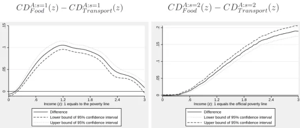
We now turn to the pro-poorness of revenue-neutral tax reforms. We first as-sume that the tax reforms are efficiency neutral, viz, that γ = 1. Recall from page 15 that with γ = 1 the tests for absolute and relative pro-poorness are equivalent. 4.3.1 Efficiency-neutral reforms involving broad classes of goods
Figure 3 presents the difference between the absolute pro-poor consumption dominance curves of Food and Transport, and this, for first and second orders of dominance. Except for rather low poverty lines, the lower bound of the confidence interval of this difference is always greater than zero, and hence a revenue-neutral tax reform that decreases food taxes and increases transportation taxes would be considered absolutely and relatively pro-poor for all P ∈ Π1(z) for a range of poverty lines extending to about 3, and for all P ∈ Π2(z) for all poverty lines, except again for a bottom range of relatively small poverty lines.
Figure 4 presents a similar difference, but this time between Food and Energy. For s = 1, the lower bound of the confidence interval is greater than zero only up to about the official poverty line. Given this degree of statistical insignificance, it is therefore not immediate that one should consider as first-order pro-poor a rev-enue and efficiency neutral tax reform that decreases food taxation and increases energy taxation — or indeed the reverse. The concern is alleviated if we move to
s = 2: the lower bound of the confidence interval is greater than zero after around z = 0.4 and up to almost 3.
Such tests of the effect of revenue and efficiency neutral tax reforms can be performed on every pair of goods. Table 2 summarizes the test results for the pairs of the three main goods. Here are some of the main findings.
• A tax reform that were to increase taxation on Transport and decrease tax-ation on Food would be absolutely and relatively first-order pro-poor over a
13Theoretically speaking, the dominance tests carried out in Section 4 must be applied over ranges varying between 0 and some z+. Statistically speaking, however, there is a general “information-less” problem in the tails of distributions that impedes such testing for values of z close to 0. Hence, statistically speaking, we must restrict the tests to a range that is lower-bounded somewhere above 0. See Davidson and Duclos (2006) for a discussion of this.
wide range of poverty lines (0.145-3 for the estimates, 0.190-2.971 for the statistically significant range).14
• A tax reform that were to increase taxation on Transport and decrease tax-ation on Energy would also be absolutely and relatively first-order pro-poor over a wide range of poverty lines (0.137-3 for the estimates, 0.211-2.953 for the statistically significant range).
• Applying statistical inference techniques can alter conclusions substantially. For instance, the estimates of Table 2 suggest that a tax reform that increases taxes on Energy and that decreases taxes on Food is pro-poor over a wide range of poverty lines (0.15 to 2.711). This is considerably shortened (0.206 to 0.925) when one focusses on the range over which the ranking of the curves is statistically significant.
• If a reform is first-order pro-poor over a range of poverty lines that starts at 0, then that range widens as we move to second-order pro-poorness — see for instance the estimates shown in the first column, where the range of poverty lines over which a rise in Food taxes combined to a fall in Energy taxes is pro-poor increases from 0-0.15 to 0-0.31 as we move from first to second-order dominance.
• This last result, however, is true only when the ranking is valid for a first-order range of poverty lines that right at 0. Table 2 shows alternative in-stances of interesting relationships between the ranges over which first-order and second-first-order dominance hold. For instance, an increase in Energy taxes and a fall in Food taxes (third column) is statistically first-order pro-poor over a range 0.206-0.925 of poverty lines; that range becomes 0.383-2.753 for second-order dominance. Increasing the order of dominance thus reduces statistical significance over the lower values of poverty lines (the lower bound increases from 0.206 to 0.383), but it increases considerably (from 0.925 to 2.753) the upper bound of poverty lines over which the rank-ing of the curves is statistically significant.
14Note that the poverty headcount at z = 0.145 is around 0.3%. Very little statistical informa-tion is thus available below that value, an indicainforma-tion of the informainforma-tion-less problem meninforma-tioned in footnote 13. It would also require a pro-poor judgement that would be almost strictly Rawlsian to reverse the pro-poor judgements implied by the tests over 0.145-3 and 0.190-2.971.
4.3.2 Efficiency-neutral reforms involving foodstuffs
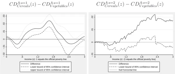
Let us now turn to the pro-poorness of revenue and efficiency neutral tax re-forms involving solely food items. Figure 5 shows for instance the difference between the pro-poor consumption dominance curve of Cereals and that of
Veg-etables for first and second orders. The results are not statistically significant.
Moreover, and as discussed above, when a reform is not statistically pro-poor within a range of poverty lines that starts at 0, the statistically insignificant range can tend to widen as s is increased. This can be seen in Figure 5 by noting that the area over which the confidence intervals overlap with the 0 line is pushed up and is wider with second-order than with first-order dominance.
The pro-poorness results involving the pairs of the three main food items are summarized in Table 3. They indicate that increasing Mexican taxes on Milk, meat
and fish to decrease taxes on Cereals and/or on Vegetables would be pro-poor, both
in terms of normative robustness and in terms of statistical significance, and this, whether we consider first or second-order dominance. The results of Table 3 also show that reforms involving any other combination of food items would not be so robustly pro-poor.
4.4 Impact of efficiency non-neutral tax reforms
We have assumed until now that tax reforms would be efficiency neutral. This assumes that the marginal deadweight loss of indirect taxation per dollar of tax raised is the same across all commodities. This is unlikely to hold since it im-plicitly assumes that compensated price elasticities are the same across all of the goods involved in the reform.
To allow for efficiency non-neutral tax reforms, assume to start with that γ = 2 — that is, that tax reforms are inefficient to the extent that each per capita dollar of tax raised on good j to finance a tax decrease on good i (see (28)) decreases per
capita welfare by 1 (namely, by γ-1) dollar. Figure 6 shows the difference between
the first-order absolute and relative pro-poor consumption dominance curves of
Food and of Energy, when the dominance curve for Energy is weighted by γ = 2.
Setting γ = 2 in that way implicitly supposes that the compensated price elasticity for Food is lower than that for Energy, and that the marginal deadweight loss from taxing Energy is thus greater than that from taxing Food.
Recall from Figure 4 that the difference between the first-order pro-poor con-sumption dominance curves of Food and of Energy was statistically positive only over a small range of poverty lines when γ was set to 1. With γ = 2, Figure 6
shows that the difference in the absolute curves is now nowhere positive. It is even in fact negative between around 0.7 and 2.2, which means that it would now be relatively pro-poor over that range of poverty lines to decrease Energy taxes and increase Food taxes.
The more inefficient it is to tax a good, the greater the tax rate that must be levied on that good to generate the tax revenues needed to decrease taxes on an-other, less price-elastic, good. If the more price-elastic good is not a luxury good, this makes the poor lose proportionately more from an inefficient tax reform than under an efficiency-neutral tax reform. This also makes increasing the price of the more price-elastic good less likely to be relatively pro-poor. Only when the price-elastic good is also a luxury good will an increase in its tax be conducive to greater relative pro-poorness. Since Energy is not a luxury good in Mexico, the greater the deadweight loss associated to taxing Energy, the more relatively pro-poor it will be to tax Food instead. This is true even though, as shown on Figure 1, Food may be less income elastic than Energy in Mexico.
Figure 6 also shows that the difference in the absolute consumption dominance curves is now everywhere positive, which also means that it is now absolutely pro-poor to tax Energy to finance a tax decrease on Food. The reverse also holds: it would absolutely anti-poor to finance a tax decrease on Energy by raising taxes on Food. This is in sharp contrast to the above results for relative pro-poorness. If the price elastic good is a normal good, the distance between the absolute loss of the rich and that of the poor for γ > 1 will be even more considerable than with an efficiency-neutral tax reform. Absolute pro-poorness of increasing taxes on the more price-elastic good is then also more likely to hold in that context.
A similar exercise is repeated in Figure 7, which shows the difference between the first-order relative and absolute pro-poor consumption dominance curve for
Cereals and that for Vegetables. The curve for Vegetables (presumably the more
price-elastic good) is being weighted by γ = 2. This can be compared to Figure 5 in which γ = 1. With γ = 2, it now possible to declare that a revenue-neutral reform that increases taxes on Cereals and decreases them on Vegetables is first-order relatively pro-poor. The reasoning is the same as before: Vegetables are not a luxury good, and it is thus better not to raise taxes on that price-elastic good. But a revenue-neutral reform that decreases taxes on Cereals and increases them on
Vegetables would be first-order absolutely pro-poor over a wide range of poverty
lines, again because, for γ > 1, that would maximize the distance between the absolute loss of the rich and that of the poor.
4.5 Trading off efficiency and distribution
The trade-off between efficiency (which is related to price elasticities) and the shape of the CD curves (which is related to income elasticities) can be usefully exemplified by the following ratio δη:si,j(z) of CD curves:
δi,jη:s(z) = CD
η:s i (z)
CDη:sj (z). (34)
Using (28) and supposing that CDη:sj (z) > 0, we then find that a revenue-neutral tax reform that reduces taxation on good i and increases taxation on good j is
η-pro-poor (η ∈ {A, R}) if and only if
δη:si,j(z) ≥ γi,j ∀z ∈
£
0, z+¤, (35)
where γi,j is the efficiency cost of taxing good j relative to good i. If CDη:sj (z) <
0, then the condition is rather that
δη:si,j(z) ≤ γi,j ∀z ∈
£
0, z+¤. (36)
When CDη:sj (z) > 0, condition (35) shows that we can interpret δη:si,j(z) as those critical efficiency ratios that must not be exceeded by γi,j for a tax reform
that reduces taxation on good i (and increases taxation on good j) to be declared pro-poor. A reverse use of δη:si,j(z) can also be made: we can interpret δi,jη:s(z) as the critical efficiency ratios that must be surpassed by γi,j for a tax reform that
reduces taxation on good j (and increases taxation on good i) to be declared pro-poor. When CDη:sj (z) < 0, condition (36) shows that we can interpret δη:si,j(z) as critical efficiency ratios that must be exceeded by γi,jfor a tax reform that reduces
taxation on good i (and increases taxation on good j) to be declared pro-poor. Figure 8 shows the δη:s(z) curves for a reform involving Food and Energy.
Let us set an upper bound z+ = 2 to the range of poverty lines. Consider first the absolute pro-poorness of a revenue-neutral reform that decreases taxation on
Food and increases taxation on Energy. Since CDA:s
Energy(z) < 0 (see Figure 2),
for such a reform to be absolutely pro-poor according to Figure 8, the efficiency cost γi,j of taxing energy relative to food must be larger than 1.7. This statistic
is given by the maximal height of the upper bound of the confidence intervals shown in Figure 8. At that maximal height, γi,j is indeed statistically greater than
δi,jη:s(z), and condition (36) is therefore statistically verified. With γi,j larger than
1.7, the absolute fall in average real income will always be larger than the fall in the poor’s real income, no matter what value of z below 2 is selected. This is
because a γi,j larger than 1.7 will always involve a sufficiently large increase in
the tax on Energy to compensate for the effect of the fall in Food taxation.
Consider then a revenue-neutral reform that increases taxation on food and decreases taxation on energy, for the same upper bound of z+ = 2. For such a reform to be absolutely pro-poor according to Figure 8, the efficiency cost γi,j of
taxing energy relative to food must be lower than 0.79. This statistic is now given by the minimal height of the lower bound of the confidence intervals, for reasons that are the reverse of those just mentioned.
A similar exercise can be carried out for relative pro-poorness, but with quite different results. Since we now have that CDR:s
Energy(z) > 0 (see Figure 1), the
condition to check is (35). A revenue-neutral reform that decreases taxation on
Food and increases taxation on Energy will be relatively pro-poor according to
Figure 8 if the efficiency cost γi,j of taxing energy relative to food is lower than
around 0.5. Conversely, a revenue-neutral reform that increases taxation on Food and decreases taxation on Energy will be relatively pro-poor if the efficiency cost
γi,j of taxing energy relative to food is greater than 4.5. When 0.5 ≤ γi,j ≤ 4.5,
the effect on relative pro-poorness of a tax reform involving Food and Energy is either statistically insignificant or normatively sensitive to the choice of indices and poverty lines between 0 and 2.
5 Conclusion
This paper develops a methodology for checking wether indirect tax reforms can be considered to be pro-poor or not. The methodology extends previous stochastic dominance techniques and enables one to characterize tax reforms on the basis of wide spectra of possible views of “pro-poorness”. This is done for both absolute and relative pro-poorness, for ranges of possible poverty lines, and for different degrees of distributional sensitivity to the differentiated impact of tax reforms across pre-reform values of welfare. Statistical inference techniques are also provided to make these tools empirically applicable.
The methodology is applied to the pro-poorness of possible reforms of Mex-ico’s indirect tax system, both across broad classes of goods and across foodstuffs. This leads to the characterizations of a number of possible pro-poor indirect tax reforms. The results also show that whether indirect tax reforms can be deemed to be pro-poor can depend to an important extent on the type of distributional and/or pro-poor views that are applied to the analysis, and that it is therefore important to make such views clear when making policy recommendations for pro-poor tax
reforms. The results further indicate that whether indirect tax reforms are pro-poor depends 1) on whether government revenue neutrality is maintained, and 2) on the size of the deadweight gains/losses incurred in the trade-off between bal-ancing efficiency and redistribution.
6 Appendix
6.1 Proof of Theorem 1
First note that, substituting (20) in (18) and (21 in (19), we obtain
∂P∗η(z) ∂ti = −Xi(q) Z ∞ 0 p(1)(y, z) CDη:1 i (y)dy. (37)
The sufficiency condition for s = 1 is proved from (37) by noting that p(1)(y, z) is negative. We then need to integrate by partsR0∞p(1)(y, z) CDη:1
i (y)dy,
Z ∞ 0
p(1)(y, z) CDη:1i (y)dy = p(1)(y, z) CDη:2i (y)¯¯∞0 (38)
−
Z ∞ 0
p(2)(y, z) CDη:2i (y) dy.
We know that CDη:2i (0) = 0 and that p1(∞, z) = 0. The first term on the r.h.s. of the above is thus nil. Consequently, equation (38) may be rewritten as
Z ∞ 0 p(1)(y, z) CDη:1 i (y)dy = − Z ∞ 0 p(2)(y, z) CDη:2 i (y) dy. (39)
Now, assume that we have: Z ∞
0
p(1)(y, z) CDη:1i (y)dy = (−1)s−2 Z ∞
0
p(s−1)(y, z) CDη:s−1i (y) dy. (40)
Integrating by parts equation (40), we get Z ∞
0
p(1)(y, z) CDη:1i (y)dy = (−1)s−2p(s−1)(y, z) CDη:s−1i (y)¯¯∞0 (41)
− (−1)s−2
Z ∞ 0
CDη:si (0) = 0 and p(s−1)(∞, z) = 0 is implied by the definition of ∞ and by (2). We can rewrite (41) as Z ∞ 0 p(1)(y, z) CDη:1 i (y)dy = (−1)s−1 Z ∞ 0 p(s)(y, z) CDη:s i (y) dy. (42)
Equation (39) obeys the relation depicted in (40). We have shown that if (40) is true then equation (42) is also true. This implies that equation (42) is true for all integer s ∈ {2, 3, ..., s − 1}. From equation (37) and (42), we get
∂P∗η(z)
∂ti
= (−1)sXi(q)
Z ∞ 0
p(s)(y, z) CDη:si (y) dy. (43) This last equation together with equation (2) proves the sufficiency of the condi-tion.
In order to establish necessity, consider the set of functions p (y, z) for which the (s − 1)th derivative (with p(0)(y, z) = p (y, z)) is of the following form
p(s−1)(y, z) = (−1)s−1² y ≤ y (−1)s−1(y + ² − y) y < y ≤ y + ² 0 y > y + ². (44) Poverty indices whose function p (y, z) has the particular above form for p(s−1)(y, z) belong to Πs. This yields:
p(s)(y, z) = 0 y < y (−1)s y < y < y + ² 0 y > y + ². (45) Imagine now that CDη:si (y) < 0 on an interval [y, y + ²] for y < z+ and for ² that can be arbitrarily close to 0. For p (y, z) defined as in (44), expression (43) is then positive and the marginal tax reform induces a marginal increase of poverty. Hence, it cannot be that CDη:si (y) < 0 for y ∈ [y, y + ²] when y < z+. This proves the necessity of the condition.
6.2 Proof of Theorem 3
d
CDs(xk; z) is a consistent estimator of CDs(xk; z) by the existence of the first
population moment of xk(y) (z − y)s−2+ and the law of large numbers. dCD
s
(xk; z)
is N0.5 consistent and asymptotically normal by the existence of the second pop-ulation moment and the central limit theorem, with asymptotic variance given by 31 by simple calculation.
6.3 Proof of Theorem 4
Note first that E h
d
CD1(xk; z)
i
= R κh(z − y) xk(y)f (y)dy. Denoting t =
h−1(z − y) and expanding around t
0 = 0, for small h this is approximately equal to E h d CD1(xk; z) i (46) ' Z κ (t) h CD1(x k; z) − thCD10(xk; z) (z) + 0.5t2h2CDd100(xk; z) (z) i dt = +0.5h2dCD100(xk; z) (z) cκ (47)
since R κ (u) du = 1,R uκ (u) du = 0, andR u2κ (u) du = c
κ. Hence, the bias
E h d CD1(xk; z) i − CD1(x k; z) is given by 0.5h2CDd 100 (xk; z)cκ.
By (32), note that dCD1(xk; z) is a sum of iid variables to which we may apply
the central limit theorem and show asymptotic normality. We also have that
N var ³ d CD1(xk; z) ´ = var (κh(z − y) xk(y)) = E £ κh(z − y)2(xk(y))2 ¤ − E h d CD1(xk; z) i2 = Z y κh(z − y)2(xk(y))2dF (y) − E h d CD1(xk; z) i2 = Z u h−2κ (u)2(x k(z − uh))2dF (z − uh) − E h d CD1(xk; z) i2 , (48)
where the last expression is obtained by substituting u for h−1(z − y). For small
h, (48) is approximately equal to Nvar ³ d CD1(xk; z) ´ ∼ = Z u h−1κ (u)2(x k(z))2f (z)du − E h d CD1(xk; z) i2 = h−1f (z) (xk(z))2 Z u κ (u)2du − E h d CD1(xk; z) i2 (49) ∼ = h−1f (z) (xk(z))2 Z u κ (u)2du (50) = h−1f (z)ck(z) Z κ (u)2du. (51)
Hence, lim N →∞Nh var ³ d CD1(xk; z) − CD1(xk; z) − h2Bk ´ = f (z)ck(z) Z κ (u)2du = Vk(z),
which concludes the proof.
References
AHMAD, E. AND N. STERN (1984): “The Theory of Reform and Indian
Indirect Taxes,” Journal of Public Economics, 25, 259–98.
ARAAR, A., J.-Y. DUCLOS, M. AUDET, AND P. MAKDISSI(2007): “Has
Mexican growth been pro-poor?” Tech. rep., Universit´e Laval.
BENNETT, S. AND L. GILSON (2001): “Health financing: designing and
implementing pro-poor policies,” Tech. rep., DFID, .
BESLEY, T.ANDR. KANBUR(1988): “Food Subsidies and Poverty
Allevi-ation,” The Economic Journal, 98, 701–719.
BOURGUIGNON, F. (2003): “The Poverty-Growth-Inequality Triangle,” in Conference on Poverty, Inequality and Growth, Paris: Agence franc¸aise
de d´eveloppement.
BRUNO, M., M. RAVALLION, ANDL. SQUIRE(1998): “Equity and Growth
in Developing Countries: Old and New Perspectives on the Policy Is-sues,” in Income Distribution and High-Quality Growth, ed. by V. Tanzi and K. C. (eds.), Cambridge: MIT Press.
CHAKRAVARTY, S. (1983): “Ethically Flexible Measures of Poverty,” Cana-dian Journal of Economics, XVI, 74–85.
CLARK, S., R. HEMMING,ANDD. ULPH(1981): “On Indices for the
Mea-surement of Poverty,” The Economic Journal, 91, 515–526.
DAVIDSON, R.ANDJ.-Y. DUCLOS(2006): “Testing for Restricted
Stochas-tic Dominance,” IZA Discussion Paper No 2047, IZA.
DOLLAR, D.ANDA. KRAAY(2002): “Growth Is Good for the Poor,” Jour-nal of Economic Growth, 7, 195–225.
DUCLOS, J.-Y. (2009): “What is “Pro-Poor”?” Social Choice and Welfare,
32, 37–58.
DUCLOS, J.-Y. AND A. ARAAR (2006): Poverty and Equity Measure-ment, Policy, and Estimation with DAD, Berlin and Ottawa: Springer
and IDRC.
DUCLOS, J.-Y. AND P. MAKDISSI (2004): “Restricted and Unrestricted
Dominance for Welfare, Inequality, and Poverty Orderings,” Journal of
Public Economic Theory, 6, 145–164.
DUCLOS, J.-Y., P. MAKDISSI, AND Q. WODON (2008):
“Socially-Improving Tax Reforms,” International Economic Review, 49, 1507– 1539.
EASTWOOD, R. AND M. LIPTON (2001): “poor Growth and
Pro-Growth Poverty Reduction: What do they Mean? What does the Evi-dence Mean? What can Policymakers do?” Asian Development Review, 19, 1–37.
ESSAMA-NSSAH, B. (2005): “A unified framework for pro-poor growth
analysis,” Economics Letters, 89, 216–221.
FISHBURN, P. ANDR. WILLIG(1984): “Transfer Principles in Income
Re-distribution,” Journal of Public Economics, 25, 323–328.
FOSTER, J., J. GREER, ANDE. THORBECKE (1984): “A Class of
Decom-posable Poverty Measures,” Econometrica, 52, 761–776.
H ¨ARDLE, W. (1990): Applied Nonparametric Regression, vol. XV,
Cam-bridge, cambridge university press ed.
KAKWANI, N., S. KHANDKER, AND H. SON (2003): “Poverty
Equiva-lent Growth Rate: With Applications to Korea and Thailand,” Tech. rep., Economic Commission for Africa.
KAKWANI, N.ANDE. PERNIA(2000): “What is Pro Poor Growth?” Asian Development Review, 18, 1–16.
KLASEN, S. (2004): “In Search of the Holy Grail: How to Achieve Pro-Poor
Growth?” in Toward Pro Poor Policies-Aid, Institutions, and
Globaliza-tion, ed. by B. Tungodden, N. Stern, and I. Kolstad, New York: Oxford
University Press, 63–94.
KOLM, S.-C. (1976): “Unequal Inequalities, I,” Journal of Economic The-ory, 12, 416–42.
LIBERATI, P. (2003): “Poverty Reducing Reforms and Subgroups
Con-sumption Dominance Curves,” Review of Income and Wealth, 49, 589– 601.
MAKDISSI, P.ANDQ. WODON(2002): “Consumption Dominance Curves:
Testing for the Impact of Indirect Tax Reforms on Poverty,” Economics
Letters, 75, 227–35.
MAYSHAR, J.AND S. YITZHAKI (1996): “Dalton-Improving Tax Reform:
When Households Differ in Ability and Needs,” Journal of Public
Eco-nomics, 62, 399–412.
MCCULLOCH, N. AND B. BAULCH (1999): “Tracking pro-poor growth,”
Tech. Rep. ID21 insights #31,, Sussex, Institute of Development Studies. PEN, J. (1971): Income Distribution: facts, theories, policies, New York:
Preaeger.
RAO, R. (1973): Linear Statistical Inference and Its Applications, New
York: John Wiley and Sons Inc.
RAVALLION, M. (2001): “Growth, Inequality and Poverty: Looking Beyond
Averages,” World Development, 29, 1803–15.
RAVALLION, M. AND S. CHEN (2003): “Measuring Pro-poor Growth,” Economics Letters, 78, 93–99.
RAVALLION, M.ANDG. DATT(2002): “Why Has Economic Growth Been
More Pro-poor in Some States of India Than Others?” Journal of
Devel-opment Economics, 68, 381–400.
SANTORO, A. (2007): “Marginal commodity tax reforms: a survey,” Jour-nal of Economic Surveys, 21, 827–848.
SON, H. (2004): “A note on pro-poor growth,” Economics Letters, 82, 307–
314.
UNITEDNATIONS (2000): A Better World for All, New York.
WATTS, H. W. (1968): “An Economic Definition of Poverty,” in Under-standing Poverty, ed. by D. Moynihan, New York: Basic Books.
WILDASIN, D. (1984): “On Public Good Provision With Distortionary
Tax-ation,” Economic Inquiry, 22, 227–243.
WORLD BANK (2002): “Globalization, Growth, and Poverty,” World bank
YITZHAKI, S.AND J. SLEMROD (1991): “Welfare Dominance: An
Appli-cation to Commodity Taxation,” American Economic Review, LXXXI, 480–96.
YITZHAKI, S. AND W. THIRSK(1990): “Welfare Dominance and the
De-sign of Excise Taxation in the Cote D’Ivoire,” Journal of Development
Economics, 33, 1–18.
Table 1: Shares (by population quintiles) of total expenditures on different goods and services
Expenditure shares in %
Quintile Poorest 2 3 4 Richest Goods and services
Food 42.99 28.88 22.61 17.20 8.04 Energy 6.13 5.09 4.45 3.87 2.64 Transport 11.74 11.90 12.09 13.32 12.42 Other goods 39.14 54.13 60.85 65.61 76.9
Shares of food expenditures
Cereals 25.88 23.91 21.20 18.95 15.90 Milk, meat and fish 28.66 37.92 41.90 45.61 46.44 Vegetables 19.30 18.30 17.63 17.86 17.66 Other food items 26.16 19.87 19.27 17.58 20.00