MECANISMES DE CONNECTIVITE FONCTIONNELLE:
UN EXEMPLE AVEC LE BISON DES PLAINES EN
MILIEU FORESTIER
Mémoire présenté
à la Faculté des études supérieures de l'Université Laval
dans le cadre du programme de maîtrise en Biologie
pour l'obtention du grade de Maître es sciences (M.Sc.)
BIOLOGIE
FACULTÉ DES SCIENCES ET GÉNIE
UNIVERSITÉ LAVAL
QUÉBEC
2010
La connectivité de l'habitat est un déterminant important de la répartition spatiale des animaux. Cette connectivité dépend de leurs comportements face aux diverses composantes de l'habitat. Notre étude évalue les mécanismes de connectivité fonctionnelle chez les bisons sauvages. Nous avons déterminé que la sélection du prochain pré visité était influencée par ses caractéristiques intrinsèques (p. ex. disponibilité des plantes) et son accessibilité (p. ex. distance). Les bisons atteignaient le prochain pré sous l'influence de la persistance directionnelle et en orientant leurs déplacements vers les trouées forestières et le pré d'arrivée. De plus, la connectivité fonctionnelle variait durant l'année. Par exemple, ils préféraient des prés offrant davantage de biomasse végétale en hiver. Notre approche permet de quantifier la probabilité d'utilisation des prés et d'établir le chemin probable pour les atteindre. Ceci permet, en retour, de définir la connectivité fonctionnelle des prés, une étape nécessaire pour mieux comprendre la connectivité du paysage.
Abstract
Habitat connectivity is an important determinant of species distribution in heterogeneous environment. Connectivity is influenced by the behavioral interactions of a species with landscape components. In this study, we evaluated the mechanisms of functional connectivity for free-ranging bison. We determined that bison selected their next meadow based on its intrinsic characteristics (e.g., plant availability) and its accessibility (e.g., distance). They reached the next meadow under the influence of directional persistence, and by orienting their movements toward canopy gaps and the target meadow. Also, functional connectivity varied among seasons. For example, bison preferred meadows with higher plant biomass in winter than in summer. Our approach provides a way to quantify the probability of selection of patches and establish the most probable path to reach them. This information constitutes the essence of patch functional connectivity, and as such, it is a fundamental step toward the understanding of landscape connectivity.
Avant-Propos
Ce mémoire de maîtrise a pour but de mieux comprendre les mécanismes de connectivité fonctionnelle dans les milieux hétérogènes en utilisant le bison des plaines du parc national de Prince Albert en Saskatchewan comme modèle d'étude. Le mémoire est composé de trois parties, soit une introduction générale, un chapitre principal écrit sous forme d'article scientifique et une conclusion générale. Le chapitre principal a été rédigé en anglais en collaboration avec mon directeur de maîtrise, le Dr Daniel Fortin, professeur au département de biologie de l'Université
Laval, et la Dre Xulin Guo, professeure associée au département de géographie de l'Université de
Saskatchewan. Cet article sera soumis à la revue scientifique Ecological Applications. Considérant mon implication dans toutes les étapes du projet, je suis la première auteure de l'article.
Remerciements
Mes plus sincères remerciements vont à Daniel Fortin, mon directeur de recherche. Il m'a d'abord donné la chance incroyable de travailler sur un projet aussi exceptionnel, qui dépassait largement ce que je pouvais seulement espérer lorsque j'étais encore étudiante au baccalauréat. Son enthousiasme contagieux vis-à-vis de la recherche et sa curiosité sans bornes ont su me motiver au-delà de mes espérances. Sa patience face à mes périodes parfois difficiles et souvent remplies d'insécurité m'a permis de mener à bien ce projet. Merci Daniel, je dois cet accomplissement à ton grand soutien...
I would also like to thank Dan Frandsen and Lloyd O'Brodovich from Parks Canada for their help with logistics in the field. Dan, your kindness and your quiet nature made me feel like everything would always be alright, and this is priceless in the field. Lloyd, you were like the grandfather 1 never had... I have learned so much from you and I believe that 1 am a better person because of the words of wisdom you always had for me. Let me tell you one last time: I could have never done it without you... Thank you for all your advice and your proteins! I also wish to thank Richard and Cheryl Crashley, for their generosity, for their kindness, for opening their home to the many bison researchers and making us feel welcome...
Merci aux nombreux assistants de terrain, particulièrement à Guillaume Bastille-Rousseau pour sa force herculéenne et son travail acharné. Merci à Élise Rioux-Paquette, Josée-Anne Otis,
Mclntire, William Parsons, Mathieu Basille, Sabrina Courant et Aurore Malapert pour leurs commentaires constructifs suite à la révision des différentes parties de ce mémoire.
Une tonne de merci pour les membres du laboratoire qui ont rendu mon séjour dans la ville de Québec des plus agréables: Ermias Azeria, Jean-Sébastien Babin, Mathieu Basille, Guillaume Bastille-Rousseau, Sabrina Courant, James Hodson, Mélina Houle, Philippe Janssen, Cheryl Johnson, Mélanie-Louise Leblanc, Jérôme Lemaître, David Pinaud et Kim Poitras. Un merci tout spécial à Sabrina, pour sa générosité sans bornes. Pour m'avoir guidée sur le terrain, pour avoir répondu à mes nombreuses questions, pour m'avoir accueillie chez elle, et pour toujours avoir ce que je n'ai pas... Tu es une personne extraordinaire. Un merci particulier pour Nicolas Courbin, Guillaume Bastille-Rousseau, Jean-Sébastien Babin, Mélanie-Louise Leblanc et Mélina Houle qui ont répondu à mes nombreuses questions...
Merci à mes amis, lecteurs assidus des chroniques de la bisonne. Vos courriels sur le terrain m'ont motivée et m'ont aussi permis de me rappeler, lors de moments plus difficiles, combien j'étais chanceuse de vivre toutes ces expériences merveilleuses. Merci d'être aussi patients lorsque je m'emballe et je parle de mes bisons sans m'arrêter... J'aurais besoin d'un mémoire complet pour pouvoir vous exprimer toute ma gratitude...
A mon amoureux, Philippe, pour sa patience (c'est loin la Saskatchewan!) et sa confiance, pour n'avoir jamais douté que je pouvais atteindre mes objectifs et pour me l'avoir rappelé lorsque j'avais tendance à l'oublier, merci mon amour... Je t'aime.
Je veux remercier mon père, d'être l'homme qu'il est, jovial, compréhertsif et attentionné. Je n'aurais pu avoir meilleur papa. À ma sœur, d'être toujours là pour moi, dans les moments joyeux comme difficiles, et pour m'avoir donné un neveu si plein de vie.
À vous tous, merci encore et, comme le dirait Wes Olsen : « puissiez-vous toujours avoir un sentier de bisons pour vous guider. »
Résumé ii Abstract iii Avant-Propos iv
Remerciements iv Table des matières 7 Liste des tableaux 8 Liste des figures 9
Introduction générale 11 La sélection des parcelles 11
La connectivité 12 La connectivité structurelle 12
La connectivité fonctionnelle 13 Les déplacements interparcelles 13
Une représentation réaliste des déplacements interparcelles 16
Objectif de l'étude 17 Chapitre Principal 19 Abstract 20 Introduction 21 Methods 23 Results 31 Discussion 40 Acknowledgments 44 Conclusion générale 45
Connectivité fonctionnelle chez le bison des plaines 45 Recommandations pour l'aménagement et recherche future 47
Table 1. Parameter estimates (coefficient ± robust standard error) of habitat variables predicting which meadow radio-collared bison of Prince Albert National Park will visit next among those available within a 2-km radius, as assessed by conditional logistic regression during
the different seasons of the year 33
Table 2. Factor loadings for the first two principal components axes (PCI and PC2) resulting from principal component analysis conducted on proportions of land cover types characterizing the areas between meadows that radio-collared bison occupied in Prince
Albert National Park and meadows that were available within a 2-km radius 35
Table 3. Factor loadings for the first two principal components axes (PCI and PC2) resulting from principal component analysis conducted on land cover type proportions around the
edge of meadows in Prince Albert National Park 36
Table 4. Candidate models assessing the influence of landscape composition, directional persistence, bias toward the target meadow, and bias toward canopy gaps along
inter-meadow trajectories of bison in Prince Albert National Park 38
Table 5. Average parameter estimates (B) with 95% confidence intervals (CI) for the most parsimonious model (Model ID 5, Table 4) of bison inter-meadow trajectories. B and CI were estimated based on 1000 randomizations of the direction of the 196 bison trails that
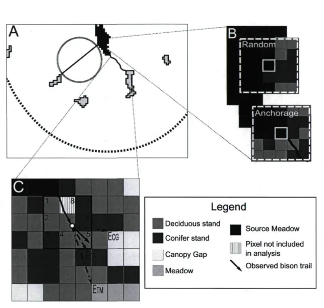
Fig. 1. Methodological design used to evaluate mechanisms of functional connectivity for plains bison in a meadow network A) Meadow selection. Ten available meadows (light gray polygons; four are visible in the section displayed) were randomly selected within a 2-km buffer zone (dashed arc) from the source meadow (black polygon), and were compared to the meadow that was actually visited next (i.e., target meadow). Meadow characteristics included: meadow area, average snow water equivalent (winter model), average plant biomass, shortest Euclidean distance between the source meadow and either a random meadow (e.g., straight black line) or the selected target meadow, and the land cover types contained within a circular buffer between the source meadow and either a random meadow or the target meadow (e.g., small-dashed circle). B) Anchorage point between bison trail and meadow. The land cover types within a 20-m buffer (dashed square) around a pixel (lower white square of 10 m x 10 m) containing a bison trail (Anchorage) were compared to the land cover types around pixels randomly selected among those without a bison trail (Random). C) Inter-meadow movement through a forest matrix. A representation of the grid-based approach describing inter-meadow trajectories from bison trails. The current location along the trail is represented by a white dot. The surrounding, pixels (10 m x 10 m) are comprised of six unused pixels (Pixels 1, 2, 3, 4, 6, and 7) and one used pixel (Pixel 5, reached by the solid black arrow representing the observed bison trail), which altogether form a stratum in statistical analysis. The animal arrived from Pixel 8, which was not included in the stratum. EDP (long-dashed arrow) represents the bearing expected according to directional persistence, ECG (dotted arrow) is the expected direction toward the nearest canopy gap, and ETM (dot-dashed arrow) is the expected direction toward the target
meadow 26
Fig. 2. Relative probability of use of meadow by radio-collared bison in Prince Albert National Park, as a function of above-ground plant biomass. Relative probabilities were calculated
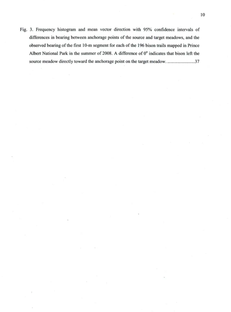
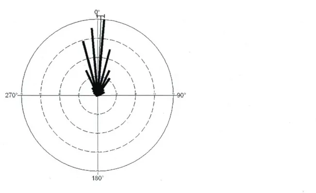
Fig. 3. Frequency histogram and mean vector direction with 95% confidence intervals of differences in bearing between anchorage points of the source and target meadows, and the observed bearing of the first 10-m segment for each of the 196 bison trails mapped in Prince Albert National Park in the summer of 2008. A difference of 0° indicates that bison left the
Introduction générale
Comprendre le lien entre les propriétés du paysage et la répartition spatiale des espèces est un thème central dans plusieurs domaines de l'écologie appliquée. Cette compréhension est essentielle, par exemple, à l'écologie des populations animales (Johnson & Seip 2008, Schick et al. 2008), l'écologie du paysage (Wiens et al. 1993), la conservation (Vane-Wright et al. 1991, Fernandez et al. 2003), et l'aménagement des écosystèmes (Eriksson et al. 2009). À une échelle plus locale, elle est aussi nécessaire à l'élaboration de stratégies d'aménagement ciblées telles que 1'implementation de réserves pour les espèces en péril (O'Brien et al. 2006), la prévention de l'invasion d'espèces non-indigènes (Diez et al. 2009) ou l'atténuation des effets des perturbations anthropiques (Courbin et al. 2009). Les patrons de répartition des espèces dans les milieux hétérogènes dépendent d'abord de la sélection de l'animal pour des parcelles de ressources. Cette sélection est cependant modulée par les qualités intrinsèques de la parcelle et par la capacité de l'animal à se rendre à ces parcelles (Arthur et al. 1996, Rhodes et al. 2005, Martin et al. 2008).
La sélection des parcelles
La sélection des parcelles d'habitat a été étudiée pour mieux comprendre la répartition des espèces (p.ex. Wiens et al. 1993, Wilmshurst et al. 2000, Johnson & Seip 2008). La sélection naturelle devrait favoriser les comportements maximisant la valeur adaptative de l'individu ("fitness") et donc, les décisions comportementales devraient être fortement influencées par le compromis entre les gains, obtenus dans la parcelle, et les coûts pour s'y rendre (Danchin et al. 2005).
La sélection des parcelles peut être influencée par plusieurs facteurs. Notamment, une espèce comme le moucherolle tchébec (Empidonax minimus), sélectionneront une parcelle d'habitat selon la présence de congénères (Fletcher 2009). D'autres, seront influencées par la quantité des ressources disponibles. Le grand brochet (Esox lucius) par exemple, peut atteindre une valeur adaptative plus élevée en sélectionnant des parcelles comportant davantage de ressources (Haugen et al. 2006). Cependant, chez les grands herbivores, le compromis entre le taux de prise alimentaire et la capacité digestive de l'animal fait en sorte qu'ils peuvent maximiser leurs gains
énergétiques en s'alimentant dans des parcelles offrant une quantité intermédiaire de biomasse végétale (Fryxell 1991, Wilmshurst et al. 2000), une théorie supportée par de multiples études empiriques (Wilmshurst et al. 1995, Bergman et al. 2001, Hebblewhite et al. 2008).
Malgré la présence d'une quantité importante des ressources de haute qualité dans la parcelle, son utilisation peut être modulée par son accessibilité (Wiens et al. 1993, Mapelli & Kittlein 2009, Schooley & Branch 2009), c'est-à-dire par son degré de connectivité avec les autres parcelles. 11 s'agit d'ailleurs d'un principe à la base des théories de la biogéographie des îles (MacArthur & Wilson 1967) et des métapopulations (Hanski 1998): la probabilité de colonisation d'une parcelle est non seulement influencée par sa taille mais aussi par son degré d'isolation avec le continent (dans le cas de la biogéographie des îles) ou avec les autres parcelles (dans le cas des métapopulations). Avec l'augmentation de la fragmentation des habitats due notamment à l'anthropisation des paysages, un nombre croissant de scientifiques cherchent à acquérir une meilleure compréhension du processus de connectivité (Taylor et al. 1993, Hanski 1998, Tischendorf & Fahrig 2000, Bélisle 2005, Crooks & Sanjayan 2006, Kadoya 2009).
La connectivité
La connectivité est un second élément ayant un impact majeur sur la répartition des espèces. L'habilité à se déplacer entre les parcelles d'habitat dans les milieux hétérogènes peut influencer directement le succès d'approvisionnement ou de dispersion des animaux et ainsi influencer leur répartition spatiale et la dynamique des populations (Goodwin 2003). Avec la perte et la fragmentation d'habitat causées par l'activité humaine, le nombre d'études sur la connectivité des parcelles a connu une augmentation quasi exponentielle depuis le début des années 1980 (Crooks & Sanjayan 2006). Malgré cette émergence, le terme connectivité et son interprétation demeurent ambigus (Bélisle 2005).
La connectivité structurelle
La connectivité entre les parcelles peut être définie sur des bases structurelles ou fonctionnelles (With et al. 1997, Tischendorf & Fahring 2000, Moilanen & Hanski 2001, Goodwin 2003, Crooks & Sanjayan 2006, Kadoya 2009). La connectivité structurelle considère
l'agrégation spatiale des parcelles et inclut donc la grandeur des parcelles et la distance qui les sépare. La connectivité structurelle d'une parcelle est souvent caractérisée par des indices comme la distance Euclidienne avec sa parcelle voisine la plus proche, l'aire totale des parcelles comprises dans une zone tampon prédéterminée, ou encore, par les modèles d'incidence fonctionnelle qui considère à la fois l'aire de la parcelle et sa distance avec toutes les autres parcelles (Kadoya 2009, Prugh 2009). Les indices sont ensuite utilisés dans des modèles visant à quantifier ou prédire la présence, l'abondance ou la survie des espèces dans cette parcelle (e.g., Lefkovitch & Fahrig 1985, Gustafson & Gardner 1996, Andersson & Bodin 2009). Selon Taylor et al. (2006), la connectivité structurelle est souvent utilisée puisqu'elle peut être quantifiée à l'aide de cartes ou de systèmes d'information géographique. Cependant, elle peut être inadéquate pour l'élaboration de stratégies d'aménagement du paysage pour une espèce particulière puisqu'elle ne considère pas les réponses comportementales de l'animal face à son milieu (Taylor et al. 2006).
La connectivité fonctionnelle
La connectivité fonctionnelle, quant à elle, implique la manière dont le paysage facilite ou gêne les déplacements des espèces entre les parcelles de ressources (Taylor et al. 1993). Il existe une reconnaissance générale à l'effet que la connectivité fonctionnelle reflète de façon plus réaliste les déplacements des animaux en considérant leurs réactions à la structure et à la composition du milieu (With et al. 1997). En effet, un individu se déplaçant entre deux parcelles ajustera ses déplacements en fonction de différentes composantes du paysage dans le but, par exemple, d'éviter certains obstacles ou d'utiliser des corridors. Pour caractériser la connectivité fonctionnelle, il est donc nécessaire d'identifier les facteurs qui influencent les déplacements des individus.
Les déplacements interparcelles
Cet intérêt croissant visant a mieux comprendre les patrons de déplacements des individus a permis l'émergence ou l'amélioration de méthodes quantitatives telles que la fonction de sélection de pas (Fortin et al. 2005a, Coulon et al. 2008, Forester et al. 2009), l'analyse mécaniste des domaines vitaux (Moorcroft & Lewis 2006, Moorcroft et al. 2006), les déplacements aléatoires biaises et corrélés (Turchin 1998, Schultz & Crone 2001, Barton et al.
2009) et les trajets de moindre coût (Adriaensen et al. 2003, Driezen et al. 2007). Ces méthodes permettent de mieux comprendre les réponses comportementales de l'individu face à son milieu mais peu d'études ont utilisé les informations acquises par ces analyses pour mieux comprendre les mécanismes de connectivité fonctionnelle (mais voir Mclntire et al. 2007).
Fonction de sélection de pas
La fonction de sélection de pas évalue l'influence de l'hétérogénéité du paysage en comparant les caractéristiques des pas observés (c.-à-d. le segment liant deux localisations successives d'un animal) et des pas aléatoires. Les pas aléatoires possèdent le même point de départ que le pas observé mais la longueur et l'angle sont généralement tirés aléatoirement de distributions représentants les habitudes de l'espèce étudiée. Par exemple, Fortin et al. (2005a) ont créé les distributions pour un animal à partir des angles et longueurs de pas des autres individus de l'étude pour éviter le problème de circularité dans les analyses. Une régression logistique conditionnelle permet, par la suite, de déterminer si les variables observées le long du pas influencent la probabilité que l'animal effectue ce pas. Cet outil a permis, entre autre, de déterminer l'influence de la topographie, des types de milieux et de la présence d'éléments anthropiques dans le paysage sur les déplacements des grands mammifères (p. ex. Fortin et al. 2005a, Coulon et al. 2008).
L'analyse mécaniste des domaines vitaux
L'analyse mécaniste des domaines vitaux utilise des outils mathématiques dérivés de modèles de déplacements corrélés des individus pour faire des prédictions sur l'utilisation de l'espace (Moorcroft et al. 2006). Moorcroft et al. (2006) ont déterminé, par exemple, que l'organisation spatiale des domaines vitaux des coyotes serait influencée à la fois par la présence de congénères et par l'abondance de proies. Ce modèle représentait de façon plus réaliste les domaines vitaux des coyotes que le modèle combinant la présence de congénères et la topographie. Cette méthode considère donc l'effet de l'hétérogénéité spatiale ainsi que des mouvements des individus pour permettre de mieux comprendre l'établissement des domaines vitaux par les animaux. Par contre, bien qu'elle informe sur l'influence de l'hétérogénéité du paysage sur la répartition spatiale des individus, ce type d'analyse n'est pas utilisé dans un contexte de connectivité fonctionnelle et ne permet donc pas de déterminer les règles qui régissent l'utilisation successive de parcelles de ressources.
Le trajet du moindre coût
L'étude des trajets du moindre coût est l'une des rares méthodes intégrant les déplacements des individus dans l'analyse de la connectivité fonctionnelle. Cette approche, basée sur des grilles de cellules dans un système d'information géographique (SIG), utilise des algorithmes informatiques pour identifier le trajet qui requiert le moindre coût cumulé pour se déplacer entre une cellule de départ et une cellule d'arrivée (Adriaensen et al. 2003). Les coûts associés à chacune des cellules sont déterminés selon les caractéristiques du paysage susceptibles d'influencer le déplacement de l'animal (Adriaensen et al. 2003, Larkin et al. 2004). Par exemple, une cellule caractérisée par une forte densité humaine pourrait avoir un coût élevé pour une espèce réfractaire au développement urbain. Cette approche a été utilisée pour identifier des corridors potentiels de dispersion pour plusieurs grands mammifères tels que le grizzly (Ursus arctos) (Walker & Craighead 1997, Chetkiewicz & Boyce 2009), l'ours noir (Ursus americanus floridanus) (Larkin et al. 2004), et le couguar (Puma concolor) (Larue & Nielsen 2008,
Chetkiewicz & Boyce 2009). Les analyses du trajet du moindre coût ne considèrent cependant pas explicitement les influences potentielles liées au biais interne, soit la tendance de l'animal à se déplacer vers l'avant, et aux biais externes du paysage qui se retrouvent plus loin que les cellules adjacentes. Ne pas considérer ces biais pourrait entraîner une interprétation erronée de l'influence de l'hétérogénéité du paysage sur les déplacements des animaux (Turchin 1998, Schultz & Crone 2001). Les modèles de déplacements aléatoires biaises et corrélés permettent cependant de considérer l'effet de la persistance directionnelle et de l'influence du paysage sur les déplacements des animaux.
Les déplacements aléatoires biaises et corrélés
Les modèles de déplacements aléatoires biaises et corrélés peuvent à la fois tenir compte de la persistance directionnelle et des biais externes. Les biais externes peuvent se refléter par l'attraction des animaux, par exemple, vers des parcelles de ressources de haute qualité (Turchin
1998, Schultz & Crone 2001) ou vers des indices olfactifs ou visuels du milieu (Zollner & Lima 1999, Moorcroft & Lewis 2006). L'ajustement des déplacements peut également se faire en fonction de la topographie (Fortin et al. 2005b, Moorcroft et al. 2006). Avec ce type de modèle, les trajectoires des déplacements peuvent refléter simultanément l'influence de la persistance directionnelle et celle des caractéristiques du paysage le long des trajets (Frair et al. 2008). Les déplacements aléatoires biaises et corrélés ont décrit avec succès les déplacements des animaux
(Schultz & Crone 2001, Fortin et al. 2005b). Néanmoins, bien que les déplacements biaises et corrélés puissent permettre de mieux comprendre la répartition des espèces (Farnsworth & Beecham 1999), les informations acquises ne sont généralement pas intégrées aux études sur la connectivité fonctionnelle.
Une représentation réaliste des déplacements interparcelles
La connectivité fonctionnelle dépend de la perception des parcelles par un animal, de l'utilisation qu'il en fait ainsi que de ses déplacements entre elles (Kadoya 2009). Les analyses de trajet du moindre coût semblent avoir été développées en parallèle avec les autres analyses quantitatives de déplacements telles que les analyses de déplacements aléatoires biaises et corrélés. Ces deux approches possèdent des avantages distincts. Les analyses du trajet du moindre coût sont attrayantes puisqu'elles offrent une représentation visuelle simple à interpréter des coûts associés aux déplacements (Driezen et al. 2007). De plus, la plupart des systèmes d'information géographique (SIG) possèdent des fonctions intégrées permettant d'identifier directement le trajet du moindre coût et facilitent donc l'utilisation de cette approche pour évaluer la connectivité fonctionnelle (Driezen et al. 2007). Cependant, les analyses du trajet du moindre coût supposent que les animaux se déplacent en pleine connaissance du chemin le moins coûteux, ce qui a été mis en doute par certains auteurs (Driezen et al. 2007, Fahrig 2007). Les analyses de déplacements aléatoires biaises et corrélés requièrent l'identification d'un point de départ mais, contrairement aux analyses du trajet du moindre coût, ils considèrent les biais interne et externes pouvant être situés plus loin que les cellules immédiates entourant la cellule de départ. Les présents modèles de déplacements aléatoires biaises et corrélés considèrent généralement un nombre limité d'éléments du paysage (Schultz & Crone 2001, Fortin et al. 2005a, Barton et al. 2009), soit généralement la persistance directionnelle et un seul biais externe susceptible d'attirer ou de repousser les individus lors de leurs déplacements. De plus, ils ont été peu utilisés pour comprendre la connectivité entre des parcelles. Les multiples biais interne et externes imposent certaines contraintes aux déplacements entre les parcelles, ce qui pourrait faire en sorte que les déplacements les plus probables ne sont pas nécessairement les moins coûteux. Par conséquent, Fahrig (2007) insiste sur l'importance d'utiliser le plus souvent possible des données de déplacements obtenues de manière empirique pour suggérer des trajets potentiels dans un réseau de parcelles de ressources. Le concept derrière ces deux méthodes offre
cependant une avenue intéressante pour comprendre les trajets empruntés par les animaux entre les parcelles de ressources. Une considération de l'influence des types de milieux ainsi que des biais interne et externes au sein d'une même analyse nous permettrait d'obtenir une représentation plus réaliste de la connectivité fonctionnelle des parcelles.
Objectif de l'étude
Pour comprendre les mécanismes de connectivité fonctionnelle basée sur la réaction de l'animal aux attributs du paysage, nous devons acquérir de l'information sur la motivation de l'animal à utiliser les parcelles (c.-à.-d. les facteurs influençant les décisions de déplacements entre les parcelles) ainsi que sur l'influence de la complexité du paysage sur le départ de la parcelle et sur la trajectoire utilisée pour atteindre la prochaine parcelle.
Notre objectif était donc d'obtenir une compréhension mécaniste de la connectivité fonctionnelle en intégrant les principes de sélection des parcelles et de déplacements. Nous utilisons un processus en trois étapes, soit 1) la décision de l'animal quant à la sélection de la prochaine parcelle à visiter, 2) l'endroit où l'animal quittera la parcelle et finalement, 3) le trajet qu'il empruntera pour atteindre la parcelle choisie. En considérant ces trois étapes, il nous sera possible d'identifier des liens probables entre des paires de parcelles tout en présentant le trajet le plus probable lors des déplacements interparcelles. Pour démontrer notre approche, nous caractérisons la connectivité fonctionnelle à travers les saisons chez le bison des plaines (Bison bison bison) se déplaçant dans le réseau de prés du parc national de Prince Albert en Saskatchewan.
D'abord, nous devons comprendre les facteurs qui influencent la sélection du prochain pré et ainsi identifier où les bisons sont les plus susceptibles de se rendre lorsqu'ils quittent un pré particulier. Pour ce faire, nous avons muni 23 femelles bisons de colliers GPS enregistrant les localisations à toutes les heures, deux jours par semaine entre mars 2005 et août 2008. Ces localisations nous permettent de déterminer l'utilisation successive des prés et de comparer les caractéristiques de chaque pré utilisé avec les caractéristiques de 10 prés choisis aléatoirement dans un rayon de 2 km. Les caractéristiques des prés susceptibles de faire varier la sélection seront celles influençant la qualité du pré ainsi que le chemin pour s'y rendre. En termes de qualité, les variables utilisées incluent la taille du pré, la biomasse végétale moyenne du pré et,
en hiver, l'équivalence en eau moyenne de la neige retrouvée dans le pré. De plus, la distance Euclidienne ainsi que la composition des forêts présentes entre le pré de départ et les prés aléatoires ou le pré choisi nous informeront sur la préférence des bisons pour les types de couverts qu'ils doivent traverser afin d'atteindre le prochain pré.
Par la suite, il s'agit de déterminer les endroits où les bisons sont les plus susceptibles de quitter un pré. En suivant systématiquement la bordure des prés, il est possible d'observer des sentiers de bisons qui se dirigent dans la forêt (c.-à.d. des points d'ancrage entre le sentier de bison et le pré). Cette recherche systématique s'est faite pour 29 prés et a permis l'identification de 196 sentiers. En comparant les types de milieux entourant ces points d'ancrage et des endroits où aucun sentier n'a été observé, il est possible de déterminer si les bisons établissent ces points d'ancrage de façon aléatoire ou préférentielle, c.-à-d. est-ce qu'un type de milieux sera sélectionné lorsque le bison quitte le pré?
Finalement, nous considérons la trajectoire empruntée par le bison entre la parcelle de départ (parcelle source) et la parcelle d'arrivée. Les sentiers observés à l'étape précédente ont été suivis à l'aide d'un GPS, jusqu'à ce qu'ils rencontrent un autre pré. Nous présentons une nouvelle approche quantitative qui permet de tenir compte à la fois de l'influence de la persistance directionnelle et des caractéristiques de l'habitat à diverses distances sur les déplacements des animaux. Nous évaluerons donc l'influence des types de milieux sur les déplacements à fine échelle (c.-à-d. en pas de 10 m), de la persistance directionnelle ainsi que des biais externes potentiels causés par l'attraction des trouées forestières et du pré d'arrivée.
Chapitre Principal
Mechanisms of functional connectivity: the case of
free-ranging bison in a forest landscape
Karine Dancose1, Daniel Fortin1, Xulin Guo2
1 Centre d'étude de la forêt and Département de biologie, Université Laval, Québec, QC,
G1V0A6, Canada
2 Department of Geography and Planning, University of Saskatchewan, 110 Kirk Hall 117
Abstract
Functional connectivity is a key determinant of animal distributions in heterogeneous landscapes. Patch connectivity depends on both patch selection and accessibility, but few studies have integrated habitat selection and movement analyses to gain a general understanding of functional connectivity. We propose to define functional connectivity by identifying which factors influence the choice of the patch that is visited next, the location from which animals leave the current patch, and the inter-patch trajectory. Twenty-three radio-collared bison were followed across the meadow network of Prince Albert National Park between 2005 and 2008. Selection of the next meadow visited over available meadows was assessed by comparing their characteristics and land cover composition of the area separating them from the departure meadow. Additionally, we used 196 bison trails originating from 29 meadows to evaluate movement rules during inter-patch travels. Bison preferred to travel in deciduous rather than in conifer stands during summer and fall, but displayed no preference during winter and spring. They also selected meadows offering higher plant biomass in winter than in other seasons. Throughout the year, meadow proximity was an important determinant of meadow selection. Inter-patch trajectory was influenced by directional persistence, as well as movement biases toward the next meadow and toward canopy gaps. Unlike the choices individuals made in selecting their next meadow, bison displayed no preference between forest stands during inter-meadow travel, indicating that functional connectivity involves hierarchical movement decisions. We showed that the behavioral determinants of functional connectivity varied over spatio-temporal scales. First, forest stand composition between meadows influenced the next target, but not the trajectory during inter-meadow travels. Second, meadow selection varied among seasons. Therefore, while structural connectivity may be immutable to such behaviorally induced changes in inter-patch movements, functional connectivity would adequately account for such modifications in animal spatial dynamics. Our study provides the tools to detect the behavioral changes necessary to bridge the gap between patch connectivity and landscape connectivity.
Introduction
Understanding the link between animal distributions and landscape properties is a central theme of ecological research. This relationship has implications in a wide range of fields, such as population ecology (Johnson & Seip 2008, Schick et al. 2008), landscape ecology (Wiens et al. 1993), and conservation biology (Vane-Wright et al. 1991, Fernandez et al. 2003). Space use patterns of animals in patchy environments strongly depend on two aspects of landscape heterogeneity: the intrinsic quality of individual habitat patches and the ability of the animal to reach these patches (/Arthur et al. 1996, Rhodes et al. 2005, Martin et al. 2008).
Animals can achieve higher fitness by making selective use of habitat patches (Morris & Davidson 2000, McLoughlin et al. 2006). Patch selection can be influenced by factors such as conspecific abundance (e.g., Fletcher 2009), presence of limited resources (e.g., Redfern et al. 2003), and the abundance of forage and its nutritional attributes (e.g., Hebblewhite et al. 2008). The use of high-quality patches, however, may be modulated by their accessibility (Wiens et al. 1993, Mapelli & Kittlein 2009, Schooley & Branch 2009), a principle central to island biogeography and metapopulation theories (MacArthur & Wilson 1967, Hanski 1998). Accessibility also determines patch use within home-ranges. For example, elk (Cervus elaphus) tend to select aspen patches in winter, unless they need to negotiate > 65° slopes to reach them, in which case they would favor open grasslands (Fortin et al. 2005a). By understanding movement decisions, we can characterize inter-patch movements and, hence, patch connectivity.
Patch connectivity can be defined on both structural and functional bases (With et al. 1997, Tischendorf & Fahring 2000, Moilanen & Hanski 2001, Goodwin 2003, Crooks & Sanjayan 2006). Structural connectivity involves the spatial contagion of habitat types, which accounts for patch size and inter-patch distances, but it does not consider behavioral processes influencing animal movement (Dunning et al. 1992, Crooks & Sanjayan 2006). In contrast, functional connectivity involves how landscapes influence the movement of organisms among patches (Taylor et al. 1993, Kadoya 2009). There is now a general recognition that functional connectivity should reflect animal spatial dynamics more faithfully by accounting for their responses to landscape structure and composition (With et al. 1997, Bélisle 2005).
A faithful characterization of functional connectivity should be based on a detailed understanding of animal movements. The growing interest in animal movement analysis has led
to the emergence and improvement of multiple quantitative methods, such as step-selection functions (Fortin et al. 2005b), mechanistic home-range analysis (Moorcroft et al. 2006), biased random walks (Schultz & Crone 2001), and least-cost paths (Adriaensen et al. 2003). Few of these methods specifically address how movement can be integrated into a framework aimed at understanding patch connectivity. Least-cost path (LCP) analysis is one of the few. This approach uses computer algorithms to identify the path which requires the least cumulative costs to move from a source to a target patch. Individual habitat units are assigned a cost, and animals are assumed to use the path of least resistance to travel between two patches. Cost attribution and the functional link between these costs and animal movement, however, are rarely validated from field observations (Fahrig 2007).
Also, LCP overlooks the potential influence of internal movement biases, such as directional persistence (i.e., the propensity for animals to keep moving ahead), and external biases toward or away from landscape features that are located farther than the adjacent habitat units (Fahrig 2007). Not accounting for these biases may lead to incorrect interpretation of the influence of habitat heterogeneity on animal movements (Turchin 1998, Schultz & Crone 2001). Biased correlated random walk models (BCRW) account for both the directional persistence and the attraction of animals to other stimuli, such as high-quality resource patches (Schultz & Crone 2001), topography (Fortin et al. 2005b, Moorcroft et al. 2006), or olfactory and visual cues (Zollner & Lima 1999, Moorcroft & Lewis 2006). Although BCRWs can be a powerful approach to understanding animal distributions (Farnsworth & Beecham 1999), this information is generally not integrated into functional connectivity studies (but see Mclntire et al. 2007).
Overall, functional connectivity depends on an animal's perceptions and use of individual patches, as well as on its movements among them (Kadoya 2009). By describing movement behavior based on the influence of multiple land cover types, together with internal and external biases, we should be able to provide a more realistic depiction of functional connectivity by identifying the most probable routes among patches (Fahrig 2007). However, because departure and arrival points will not be automatically identified, as with the cumulative cost trajectory determined through LCP, we need to determine whether animals select these two locations or place them randomly along patch edges. In summary, to understand mechanisms of functional connectivity based on the animal's responses to landscape features, we need to gain information
on factors influencing patch selection, trail-patch anchorage locations, and movement trajectories toward the target patch.
Our objective was to develop a mechanistic understanding of functional connectivity by integrating patch selection and inter-patch movement decisions. We proposed a three-step approach: first, we identified factors influencing the probability of a patch being visited next; second, we determined the locations from which animals are most likely to leave the current patch; and third, we evaluated the determinants of movement trajectories between the current and target patches. Inter-patch trajectories were assessed using a grid-based approach that can account for internal biases, as well as external movement biases caused by the characteristics of adjacent and remote cells. The three-step approach was implemented based on extensive spatial information on plains bison (Bison bison bison) traveling among meadow patches in Prince Albert National Park, Saskatchewan, Canada.
Methods
Bison population and study area
The bison population of Prince Albert National Park (53°44'N, 106°40'W) was estimated at 385 individuals in 2006 (Fortin et al. 2009). The bison range is dominated by a matrix of conifer and deciduous stands (85%), interspersed with meadows (10%) and water bodies (5%). Bison strongly select meadows rich in grasses and sedges (Fortin et al. 2003). In this context, meadows can be considered as high-quality patches imbedded within a forest matrix.
Field data collection
Two sets of data were collected in the field. First, we followed radio-collared bison to identify meadows that were successively visited. Second, bison trails were mapped from field surveys to identify trail-meadow anchorage points (i.e., the locations where bison trails meet the meadow edge), and trail trajectories between meadows.
Radio-collared bison
Global positioning system (GPS) collars (4400M from Lotek Engineering, Newmarket, Ontario, Canada) were installed on 23 female bison. Individuals were followed for periods ranging from 82 to 997 days (mean = 454 days) between March 2005 and August 2008. Differences in period lengths were due to animal mortality, collar malfunctions, or battery exhaustion. GPS locations were taken every three hours five days a week and every hour two
days a week, but only hourly locations were used to identify meadows that were successively visited.
Bison trails
Bison are gregarious animals, which travel within extensive networks of trails (McHugh 1958). In summer, bison trails are large, conspicuous, and denuded of vegetation. They can be easily distinguished from those of other ungulates by their large rounded hoof prints and presence of faeces (Elbroch 2003), although other species also use bison trails. During the summer of 2008, bison trails (number of trails: 9.2 ± 1.1 [mean ± SE] trails per meadow; range: 2-28 trails, N = 196) were systematically located by walking around the edge of 29 meadows (meadow area: 8.5 ± 1.94 ha; range: 0.08-33.7 ha). All trails were followed using a handheld Global Positional System unit (GPS76, Garmin International, Inc., Olathe, Kansas, USA) until they reached another meadow. The information was then transferred to a Geographic Information System (GIS, ArcGIS 9.3, Environmental Systems Research Institute, Redlands, California, USA).
Remote sensing and geographic information system of bison habitat
A supervised classification of a SPOT5 multispectral image (August 2008; 10 m x 10 m pixel resolution) was performed to define landscape attributes over the bison range, based on 310 random field locations. Each field location was taken in a 30 m x 30 m area composed of a single land cover type. The resulting map depicted, with an accuracy of 89% (N =310), six different landscape covers: WATER, AGRICULTURE, CONIFER stands, DECIDUOUS stands, MIXED stands, and open areas. Open areas were subsequently transformed into two categories: MEADOW and canopy GAP. A meadow was an aggregation of at least five pixels (> 0.04 ha), whereas a gap included fewer than five aggregated pixels. Groups of MEADOW pixels were then transformed into a polygon layer. The area of each of these patches was estimated using Hawth's analysis tools for ArcGIS (Beyer 2004).
To obtain a general indication of plant abundance over the bison range, we followed the example of Anderson et al. (2005) and sampled vegetation when the biomass was at its highest (i.e., August 2008). We collected five vegetation samples of 0.25 m2 of above-ground vegetation
at 24 sites of 30 m x 30 m, one in the center and four approximately 5 m from each edge toward the center. Samples were oven-dried to constant mass. We then established a relationship between total above-ground dry biomass and the Normalized Difference Vegetation Index
(NDV1): NDVI = (NIR - RED)/(N1R + RED), with surface reflectance values for near-infrared (NIR) and red bands (RED) that were obtained from the SPOT5 image. The relationship between total dry biomass (kg/m2) and NDVI was as follows: Total dry biomass = 1.52 x NDVI - 0.77,
(R2 = 0.47, N = 24, P < 0.01). This relationship was used to estimate average biomass in each
meadow.
During winter, bison access their food by removing snow with their heads. This obstacle implies extra energy expenditure, and deep or dense snow can therefore decrease meadow quality. We characterized snow conditions in meadows across the bison range, based on the snow model described by Fortin et al. (2009). In summary, snow depth and density was measured every 10 m along a 70-m transect located in each of 18 open areas during the winters of 2006 (4 surveys), 2007 (5 surveys), and 2008 (4 surveys). Snow depth was recorded and the snow contained in a metal tube of known diameter was weighed with a spring scale to obtain snow density. Snow water equivalent (SWE) was then calculated from the product of snow depth and density. An inverse distance weighting function was used to extrapolate SWE to unsampled areas (Schloeder et al. 2001). Model cross-validation indicates a robust relationship between predicted and observed values (R2 = 0.76). A different map was created for every snow survey.
Because snow surveys were taken approximately every two weeks, a given snow map was associated with all observations of radio-collared bison that had been taken from one week prior to the snow survey to one week after the survey. Snow maps were used to estimate SWE in the meadows from January to mid-March.
Analysis of functional connectivity Meadow selection
We used sequences of GPS locations ( 1 -h relocation interval) from radio-collared bison to characterize their successive use of meadows. We first identified a meadow with at least one bison GPS location (i.e., the source meadow), and then determined which meadow was visited next (i.e., the target meadow). We then characterized this target meadow, together with 10 meadows randomly chosen (random meadow) within a 2-km radius of the source meadow (Fig.
I
Legend
| Deciduous stand
1 Source Meadow | Conifer stand
™ Pixel not included Mill jn a n a|ySjS
J Canopy Gap
™ Pixel not included Mill jn a n a|ySjS
• j Meadow > y Observed bison trail
Fig. 1. Methodological design used to evaluate mechanisms of functional connectivity for plains bison in a meadow network. A) Meadow selection. Ten available meadows (light gray polygons; four are visible in the section displayed) were randomly selected within a 2-km buffer zone (dashed arc) from the source meadow (black polygon), and were compared to the meadow that was actually visited next (i.e., target meadow). Meadow characteristics included: meadow area, average snow water equivalent (winter model), average plant biomass, shortest Euclidean distance between the source meadow and either a random meadow (e.g., straight black line) or the selected target meadow, and the land cover types contained within a circular buffer between the source meadow and either a random meadow or the target meadow (e.g., small-dashed circle). B) Anchorage point between bison trail and meadow. The land cover types within a 20-m buffer (dashed square) around a pixel (lower white square of 10 m x 10 m) containing a bison trail (Anchorage) were compared to the land cover types around pixels randomly selected among those without a bison trail (Random). C) Inter-meadow movement through a forest matrix. A representation of the grid-based approach describing inter-meadow trajectories from bison trails. The current location along the trail is represented by a white dot. The surrounding
pixels (10 m x 10 m) are comprised of six unused pixels (Pixels 1, 2, 3, 4, 6, and 7) and one used pixel (Pixel 5, reached by the solid black arrow representing the observed bison trail), which altogether form a stratum in statistical analysis. The animal arrived from Pixel 8, which was not included in the stratum. EDP (long-dashed arrow) represents the bearing expected according to directional persistence, ECG (dotted arrow) is the expected direction toward the nearest canopy gap, and ETM (dot-dashed arrow) is the expected direction toward the target meadow.
We characterized each meadow by its area, average plant biomass (kg/m2), squared biomass
(second order, to test for a possible quadratic relationship between use and plant biomass, Wilmshurst et al. 1995) and, for the winter model, the average SWE of the meadow. We centred biomass estimates to avoid muticollinearity in subsequent statistical models. We also determined the Euclidean distance linking the edge of the source meadow and the edge of target or random meadows. To account for the environmental characteristics of the area between the source and the target meadows or the source and the random meadows, we created a circular buffer with a diameter equal to the shortest distance linking a given pair of meadows and centred on the midpoint of this vector (cf., Johnson et al. 2002b; Fig. 1A). The proportion of the different land cover types within the buffers was estimated. Because the proportions of the land cover types were non-independent, we used a principal component analysis (PCA) to reduce the dimensions of the data to two independent components (PCI and PC2) that identified the major spatial gradients among the land cover types (Graham 2003).
We contrasted the characteristics of target (score = 1) and random (score = 0) meadows with conditional logistic regression (Compton et al. 2002, Fortin et al. 2005a), for which each stratum was comprised of one target meadow and its 10 associated random meadows. Models were built for each season (Summer, June-August; Fall, September-November; Winter, January to mid-March; Spring, mid-March to the end of May). Winter did not include December because of the lack of snow data. Model robustness was evaluated for each season with &-fold cross-validation for conditional logistic regression (Fortin et al. 2009). For validation, each model is build utilizing 80% of randomly selected stratum and, using the parameter derived from this portion of the data, the probability of use (w(x)) is evaluated for the remaining 20% of the stratum. A high Spearman rank correlation (rs) indicates high model robustness (cf., Fortin et al. 2009). The
process was repeated 1000 times for this study. We present the average r. ( r. ) resulting from the 1000 randomizations.
Anchorage points between bison trails and meadows
To evaluate whether or not bison trails were randomly established along meadow edges, we calculated the proportion of the different land cover types (i.e., deciduous stands, conifer stands, mixed stands, meadows, canopy gaps, and water) in a 20-m buffer around pixels (i.e., 24 adjacent pixels) where a trail connects the meadow (i.e., anchorage point, coded as 1). For each trail found at the edge of a meadow, we also randomly selected pixels along the meadow edge where trails were absent (i.e., coded as 0) and characterized the proportion of land cover types around them (Fig. IB). When there were sufficient pixels of meadow edge, we randomly selected five pixels without trail for each pixel with trail; otherwise, all pixels without trails were included in the analysis. Again, because the proportions of the land cover types were non-independent, we used a principal component analysis (PCA) and estimated PC 1 and PC2 scores. We then used a conditional logistic regression to contrast PC scores of pixels with- and without-trails. Because each meadow was characterized by more than one bison trail, all anchorage pixels and associated random pixels of a given meadow were grouped into the same stratum in the regression (i.e., each stratum had multiple Is, each representing a bison trail, with multiple 0s). This approach accounted for the statistical non-independence of all the trails reaching a given meadow.
Estimated parameters of the model were used to calculate the probability of finding an anchorage point at any given pixel along the meadow edge (i.e., random and anchorage points). With a robust model, pixels with the highest probabilities should have an actual anchorage point (i.e., be coded as 1). We thus evaluated the number of times that pixels with the highest probabilities were anchorage points. This was done separately for each of the 29 meadows; for example, for a meadow with five anchorage points, we identified the five pixels with the highest probabilities and determined whether they had an anchorage point. We then reported the percentage of times that anchorage points were successfully identified. A high percentage is indicative of a robust model. Additionally, to evaluate the improvement of our model over random establishment of anchorage points, a null model that assumed completely random establishment of anchorage points on the meadow's edge (i.e., Is were randomly attributed among the pixels) was also constructed. Random assignment of anchorage points was repeated 1000 times, and the mean percentage is reported for the null model.
Inter-meadow movements through the forest matrix
We developed a grid-based approach to assess the simultaneous effects of land cover type preferences and movement biases on animal movement. We considered that biases of bison movement could include directional persistence, a bias toward the target meadow, and a bias toward canopy gaps, which could be used as stepping stones during inter-meadow travel. Bison trails were split into 10-m segments (i.e., 10-m steps). The current location was surrounded by eight pixels: one pixel where the animal came from, one that was subsequently used, and six unused pixels. A choice set (a stratum) thus includes the used (coded as 1) and the six related unused pixels (coded as 0). We compared the characteristics of used and unused pixels (Fig.lC).
Pixels were characterized through a set of dummy variables, each representing a given land cover type (i.e., DECIDUOUS stand, CONIFER stand, MIXED stand, MEADOW, or canopy GAP). WATER was not included in the analysis because it was unavailable along the bison trails. We also considered that when an animal is exhibiting directional persistence, the expected
direction of the current step, Eop(9t), equals that of the previous step: Eop(Ot) = 6.-1. We calculated
the cosine of the difference between EDP(0,) and the direction toward each of the seven
neighboring pixels (XDP). For example, Pixel 2 would have XDP value of cosine 125° (i.e., -0.57),
whereas Pixel 3 would be assigned a XDP value of cosine 85° (i.e., 0.09; Fig 1C).
The expected step direction in the case of a bias toward the target meadow (ETlvi(0t))
corresponds to the bearing direction between the current location and the target meadow (Fig. 1C). Each pixel of a stratum was then assigned a value corresponding to the cosine of the
difference between ETM(OI) and the bearing of the vector going from the current location to the
pixel (XTM)- For example, Pixel 1 would be assigned a XTM value of cosine 170° (i.e., -0.98) and
Pixel 2, a XTM value of cosine 125° (i.e., -0.57). Because the strength of the bias could vary with distance (Barton .et al. 2009), we also accounted for the Euclidean distance (DJM) to the target
meadow by multiplying XTM by DTM° (no distance effect), DTM°'5 (effect increasing with
distance), or DTM"° 5 (effect decreasing with distance) (Eq. 1 ).
Finally, we also considered an external bias toward canopy gaps. The expected step direction
toward canopy gaps (ECG(OI)) was the bearing direction between the current location and the
nearest canopy gaps (Fig. 1C). Because gaps could be used as stepping stones while traveling toward the target patch, we assumed that bison would be influenced only by canopy gaps
only be within 90° on either side of the previous step bearing direction). Each pixel of a stratum
was then assigned a value (XCG) corresponding to the cosine of the difference between ECG(0I)
and the bearing of the vector going from the current location to the pixel. We also accounted for potential changes in the strength of this external bias with the Euclidean distance (DCG) to the canopy gap (Eq. 1).
We used conditional logistic regression to evaluate the combined influence of movement biases (i.e., directional persistence, bias toward target meadow, and bias toward canopy gaps) and land cover types on the probability of pixel use. The regression model was based on a paired design whereby each pixel actually used (i.e., pixel part of the trail, coded as 1) was associated with the six unused pixels available from that location (pixels adjacent to the trail, coded as 0s) to form a stratum. Robust 95% confidence intervals of regression parameters were estimated using generalized estimating equations (GEE; Craiu et al. 2008, Koper & Manseau 2009) to control for the lack of independence in the information along each trail. All strata associated with a given trail were assigned to a given cluster in the GEE analysis.
We contrasted the relative empirical support provided by seven candidate models. The first three models (wmove(x)), Models 1 to 3, included only variables of movement parameters:
wm0ve(x) = exp(pDPXDP + PTMXTMDTM0 + PCGXCGDCG0), ( 1 )
To investigate distance effects on the strength of external biases, we tested a model with no distance effect (c = 0, Model 1), as well as models based on the two different functional forms of distance effects: a decreasing effect (c = -0.5, Model 2), and an increasing effect (c = 0.5, Model 3).
The next model (wcover(x)), Model 4, included only dummy variables representing the land
cover types:
wcover(x) = exp(PcoNiFERXcoNiFER +PDECIDUOUSXDEC]DUOUS+PMEJ\DOWXMEADOW + PGAPXGAP), (2)
with MIXED stands being the reference category.
The last three models included both land cover types and movement parameters with varying
ww_-/{x) = winoVe(x) x wcmer(x) = exp(pDpXDp + PCGXCGD0 +...+ PCONIFERXCONIFER +■••+
PGAPXGAP), (3)
where c varied as described above to create three additional candidate models: no distance effect (c = 0, Model 5), decreasing effect (c = -0.5, Model 6), and increasing effect (c = 0.5, Model 7).
Because trails could be used in both directions, all estimates of bearing direction associated with potential internal and external biases could vary depending on which way we considered the animals to be moving. To get a general assessment of factors influencing inter-patch movement trajectories, we randomly selected a direction for each of the 196 bison trails, and estimated the regression parameters. We repeated this randomization procedure 999 times and reported average regression parameters with 95% confidence intervals for the 1000 runs. For each randomization, the seven candidate models were contrasted based on the Quasi-likelihood under Independence Criterion (QIC; Pan 2001, Craiu et al. 2008), and we reported the percentage of the 1000 runs for each model that had the lowest QIC. The model with the lowest QIC was considered the best one among the seven candidate models and, therefore, the model with the highest percentage was considered to have received the most empirical support.
Results
Meadow selection
Models of meadow selection revealed that multiple habitat characteristics influenced which meadow bison visited next. In all seasons, bison leaving a meadow were more likely to end up in a large rather than a small meadow, among those that were available within a 2-km radius (Table 1). This effect could have been expected simply by chance, but needed to be accounted for before assessing the response of bison to other habitat variables. Throughout the year, bison were also more likely to visit meadows closer to their current location. Snow water equivalent (SWE) in meadows did not influence its selection.
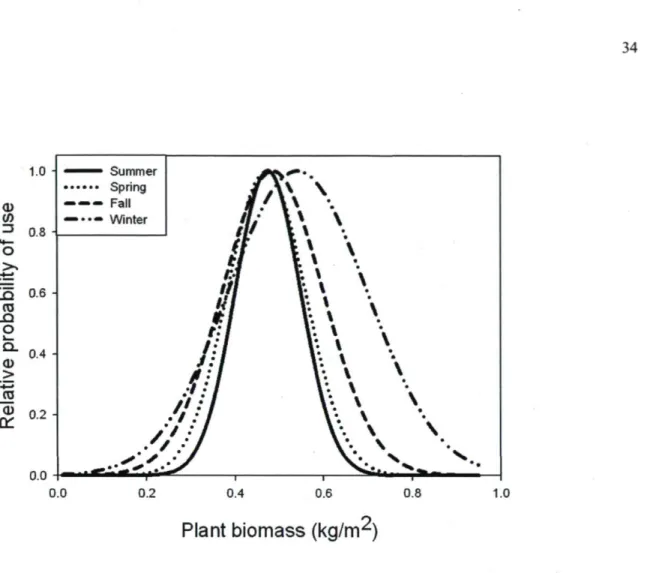
Bison were most likely to visit a meadow offering an intermediate amount of plant biomass (Fig. 2) within the estimated range (0.02-0.75 kg/m2). The relative probability of use of meadows
was highest when biomass was approximately 0.48 kg/m2 during snow-free seasons, and 0.54
source and target meadow. The first two PCA axes explained 63% of the variance in the land cover types located between the source meadow and the available ones. PCI reflected a gradient of forest types from deciduous to conifer stands, whereas PC2 mostly represented a water gradient (Table 2). In winter and spring, land cover types did not significantly affect selection of the next meadow (Table 1). In fall and summer, however, bison were more likely to travel toward meadows separated from their current location by a high proportion of deciduous stands than by conifer stands. In summer, bison avoided areas comprised of a high proportion of water (i.e., negative association with PC2). Models of meadow selection were robust to cross-validation during any season (r. > 0.84, Table 1).
o 'JO d d o 'JO ■7 V V V V 35 DQ _) TS | E 00 o o r i p v O i n i / - ) TS | — 00 o n r i p O O .—< CJ oo u o , 1 d d d d 0 0 O g w oo o -H -H -H +i -H l 0 0 o '5b -H -H m oc oc O 1 d _o C Q . r- r-oc o O oc ro "rô o o d 1 d N E d d r i i
a
c o o •a " 5 __ __ c o o N C i r > __ r i O i n £ " 5 c o tt, o i n O n r- o 0 0 £ CJ o d d d d d O X > N X J V V Le -a w5
S u r-t û j o JO e _ t * ■ * oo oc oc l O g ( De»
o ro d o o n 0 0 rjo JOe»
oo -H o _ _ ■ d d d o \ D «_> C_ oo -H -H C N -H r^ -H ro o -H ro -H -H -H 0 0 d S c__ ro r~ ro O — ] *""■ ga 3 o d d d d o 1_u
T3 i x ro.s
E , ! __ __ ro E O o o n O N o > t tt, O o o o r t o 1 r - l tt, o d d d d d c .v
v V V -S C ro x !£ t * -o'1
" 3 PL o ao r- o N O » o n .—-I M u W o -H o o o d r--' d d d O t X _ro OO -H o -H o o o +1 c -H -H O C +1 -H O N 1 1 oo d T .i
' 3 > c . c a . o -H o o o O N r i O N ro d i o d O C rs -a U 1 c j o « O ta -C ta — c/0 M o O o r t , | o 3 c tt, o C o O o o 1 X O o E a tt, o V d V d V d d d V -H >-. h * C £ E 3 oo O N eu c fc_ £ E 3 oo , oc oc N O N C ** '•7. C . u > N £ E 3 oo 00 o © ~ d O d d d i r > '> u 00 -H -H -H -H -H -H 1 O S O o X 4 - * -H oo C N ■ 3 - ■ t U - l n O O o*5
<4_ C Q . o O N — —' 1 ! » B l*5
O o O C ro O O r i U _* WD t O N 1 1 • ro E t -C3 0 -c O V3 1 t a u . U « J E H 73 c o .ta. C3 C3 _) c E i—s"
o o ro TJ t a u . U « J E Hz
ë
_.! r i •JO ' 5 o C .—. TJ o èa "rô > i --c_ _> -5 ■jj E o 15 S 'JO ro E O XJ +—' c ro CL U o E o TJ èa 'JO C L U X J S r -X ) < u CJ ç CL o x 60 ç *£_ 3 ■ o 4 > "ca > o U 'es J = c . • J — < ■jj E o 15 S 'JO ro E O XJ +—' c ro CL i JO CS § | '3 "S Q 5b ro t -Sb i -ro S OJ CJ c ro v . Q u E ç oo S CJ - vGO 1.0 0.8 O _5 ro .a o 0.6 ■ " " 0.4 >
S.
02 0.0 ^ ^ ^ Summer *""•. / / _N ^ — — - Fall / /Y *
_ . . _ . winter'f
'f
\ * *
\ \ \
rf\ \ \
M\ t
\ \ \
W
l \ \
* /l \ \
'•7
1" \
/ / /1" \
In
1" \
'in
• f X IV.
x
• / / /
V * N
• / / /
V ^
- * • ■ ' . • _ _ / V - N v._r.V_>V,>^ ,
>fc^. * » ^ 0.0 0.2 0.4 0.6 0.8 1.0Plant biomass (kg/m
2)
Fig. 2. Relative probability of use of meadow by radio-collared bison in Prince Albert National Park, as a function of above-ground plant biomass. Relative probabilities were calculated using the seasonal models presented in Table 1.
Table 2. Factor loadings for the first two principal components axes (PCI and PC2) resulting from principal component analysis conducted on proportions of land cover types characterizing the areas between meadows that radio-collared bison occupied in Prince Albert National Park and meadows that were available within a 2-km radius.
Land cover type Conifer-deciduous gradient Water gradient
PCI PC2 Proportion of water 0.09 0.84 Proportion of conifer stands 0.58 -0.03 Proportion of deciduous stands -0.64 -0.23 Proportion of mixed stands 0.49 -0.41 Proportion of canopy gaps -0.02 0.27 Notes: PCI and PC2 have eigenvalues of 2.0 and 1.2, respectively; collectively, they explained 63% of variation in the correlation matrix.
Anchorage points of bison trails
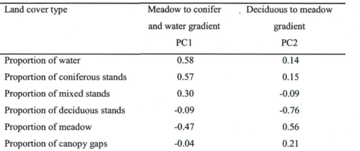
We characterized the area surrounding the anchorage points of bison trails, with the first two PCA axes, which altogether explained 57% of the variation in land cover types. The first principal component (PC 1 ) mostly distinguished meadows from conifer stands and water bodies, whereas the second component (PC2) represented a gradient from deciduous stands to meadows (Table 3). The probability of finding trail anchorage points along a meadow edge was influenced by both PCI ((3 ± SE = 0.13 ± 0.06, N = 250, P = 0.02) and PC2 (p ± SE = -0.74 ± 0.07, N = 250, P < 0.0001). PCI indicated that anchorage points are more likely to be found in areas with a low proportion of meadows, and a high proportion of coniferous stands and water bodies. We suggest that this relationship with PC 1 was largely driven by a response to meadows, and had little to do with conifer stands and water bodies. First, a univariate analysis confirmed that the probability of finding an anchorage point at a given location decreased with the proportion of meadow around that location (P ± SE = -5.55 ± 0.56, N = 250, P < 0.0001), but was independent of conifer stands (p ± SE = -3.95 ± 2.87, yV= 250, P = 0.16) or water bodies (P ± SE = -1.80 ± 1.69, N = 250, P = 0.28). Second, PC2 also indicated that trail anchorage points were selectively placed in areas characterized by a small proportion of meadow. PC2 further revealed that trails were most likely
to connect meadows in areas with a high proportion of deciduous stands. The presence of deciduous stands at anchorage points was confirmed through a univariate analysis (P ± SE = 5.85 ± 0.60, N= 250, P < 0.0001).
Our model correctly identified pixels with a trail anchorage point 39% of the time, which exceeds random expectations (mean 21%; range [15-28%]). Model parameters thus significantly improved our ability to predict where bison trails connect to meadows.
Table 3. Factor loadings for the first two principal components axes (PCI and PC2) resulting from principal component analysis conducted on land cover type proportions around the edge of meadows in Prince Albert National Park.
Land cover type Meadow to conifer , Deciduous to meadow and water gradient gradient
PCI PC2
Proportion of water 0.58 0.14
Proportion of coniferous stands 0.57 0.15 Proportion of mixed stands 0.30 -0.09 Proportion of deciduous stands -0.09 -0.76
Proportion of meadow -0.47 0.56
Proportion of canopy gaps -0.04 0.21
Notes: PCI and PC2 have eigenvalues of 1.81 and 1.61, respectively; collectively, they explained 58% of the variation in the correlation matrix.
Inter-meadow movement through forest matrix
We estimated the difference between the bearing direction at a trail anchorage point and the arrival point in the next meadow, together with the bearing direction of the first 10-m segment of the trail. This difference in bearing direction averaged 2.54° ± 1.34° (mean ± SE, N = 392), with a 95% confidence interval that included 0° (Fig. 3). The length of the mean vector (r) was 0.9 indicating a high concentration around the mean and the distribution of the differences in bearing direction was not uniform (Rayleigh test of uniformity, P < 0.001 TV = 392). Bison thus tended to leave directly in the direction of their arrival point in the target meadow. Anchorage points of bison trails were rarely located in the areas corresponding to the shortest Euclidean distance
between the two meadows. The Euclidean distance that linked the anchorage points of the two meadows was 135.9 ± 25.3% longer (mean ± SE; median: 23.8%, N = 196, range: 0 - 2252.1%) than the minimum distance between the two meadows. This indicates that, although bison leave directly toward the target meadow, they do not use the shortest trajectory to reach it.
2701
ISO-Fig. 3. Frequency histogram and mean vector direction with 95% confidence intervals of differences in bearing between anchorage points of the source and target meadows, and the observed bearing of the first 10-m segment for each of the 196 bison trails mapped in Prince Albert National Park in the summer of 2008. A difference of 0° indicates that bison left the source meadow directly toward the anchorage point on the target meadow.
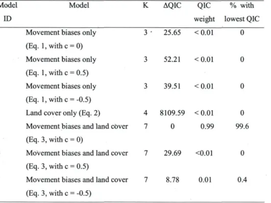
Among the seven candidate models that investigated the factors shaping the trajectory of bison trails, Model 5 received the greatest empirical support. Its QIC was the lowest 99.6% of the time (N = 1000). Model 5 implied that bison trail trajectories resulted from the influences of land cover types, directional persistence, and external biases without a distance effect (average QIC weight > 0.99, N = 1000; Table 4). Models that only accounted for land cover types or movement biases had poor empirical support (QIC weight < 0.01, in both cases). Also, considering that
effects of external biases increased or decreased with distance did not improve model fit (QIC weight < 0.03 for Models 3,4, 6 or 7, Table 4).
Table 4. Candidate models assessing the influence of landscape composition, directional persistence, bias toward the target meadow, and bias toward canopy gaps along inter-meadow trajectories of bison in Prince Albert National Park.
Model ID
Model K AQIC QIC % with
weight lowest QIC 1 Movement biases only
(Eq. l,withc = 0) 2 Movement biases only
(Eq. 1, withe = 0.5) 3 Movement biases only
(Eq. 1, withe = -0.5) 4 Land cover only (Eq. 2)
5 Movement biases and land cover (Eq. 3, with c = 0)
6 Movement biases and land cover (Eq. 3, with c = 0.5)
7 Movement biases and land cover (Eq. 3, with c = -0.5) 3 • 25.65 < 0.01 0 3 52.21 <0.01 0 3 39.51 <0.01 0 4 8109.59 <0.01 0 7 0 0.99 99.6 7 29.69 <0.01 0 7 8.78 0.01 0.4 Note: AQIC, QIC weights and % with lowest QIC are calculated, based on the average QIC of
1000 randomizations of directionality in the 196 bison trails.
The top-ranking model (model 5) indicated that, along their paths, bison were not more likely to use deciduous or conifer stands than mixed stands (Table 5). Trails also bypassed meadows that were located between the source and target meadows. Meadow avoidance simply pointed out that, although bison tended to select meadows that were in relatively close proximity (Table 3), trails did not always connect the two nearest meadows. We found that bison trails were more likely to go through canopy GAPS than other land cover types. Moreover, we detected positive