This is an author-deposited version published in :
http://oatao.univ-toulouse.fr/
Eprints ID : 5624
To link to this article : DOI: 10.1109/TSP.2012.2190066
URL : http://dx.doi.org/10.1109/TSP.2012.2190066
O
pen
A
rchive
T
OULOUSE
A
rchive
O
uverte (
OATAO
)
OATAO is an open access repository that collects the work of Toulouse researchers and
makes it freely available over the web where possible.
To cite this version :
Kail, Georg and Tourneret, Jean-Yves and Hlawatsch, Franz
and
Dobigeon, Nicolas
Blind deconvolution of sparse pulse sequences
under a minimum distance constraint: a partially collapsed Gibbs
sampler method
.
(2012) IEEE Transactions on Signal Processing,
vol. 60 (n° 6). pp. 2727-2743. ISSN 1053-587X
Any correspondence concerning this service should be sent to the repository
administrator:
[email protected]
Blind Deconvolution of Sparse Pulse Sequences
Under a Minimum Distance Constraint: A Partially
Collapsed Gibbs Sampler Method
Georg Kail, Jean-Yves Tourneret, Senior Member, IEEE, Franz Hlawatsch, Fellow, IEEE, and
Nicolas Dobigeon, Member, IEEE
Abstract—For blind deconvolution of an unknown sparse
se-quence convolved with an unknown pulse, a powerful Bayesian method employs the Gibbs sampler in combination with a Bernoulli–Gaussian prior modeling sparsity. In this paper, we extend this method by introducing a minimum distance constraint for the pulses in the sequence. This is physically relevant in ap-plications including layer detection, medical imaging, seismology, and multipath parameter estimation. We propose a Bayesian method for blind deconvolution that is based on a modified Bernoulli–Gaussian prior including a minimum distance con-straint factor. The core of our method is a partially collapsed Gibbs
sampler (PCGS) that tolerates and even exploits the strong local
dependencies introduced by the minimum distance constraint. Simulation results demonstrate significant performance gains compared to a recently proposed PCGS. The main advantages of the minimum distance constraint are a substantial reduction of computational complexity and of the number of spurious components in the deconvolution result.
Index Terms—Bernoulli–Gaussian prior, blind deconvolution,
Markov chain Monte Carlo method, partially collapsed Gibbs sampler, sparse deconvolution.
I. INTRODUCTION
T
HE problem of blind deconvolution (BD) arises in many applications where some desired signal is to be recovered from a distorted observation, e.g., in digital communications [1]–[5], seismology [6]–[9], biomedical signal processing [10]–[13], and astronomy [14], [15]. The BD problem is ill-posed since different input sequences and impulse responses can provide the same observation. As a consequence, additional assumptions or constraints have to be considered in order to re-duce the number of solutions. Examples of constraints that haveG. Kail and F. Hlawatsch are with the Institute of Telecommunications, Vi-enna University of Technology, A-1040 ViVi-enna, Austria (e-mail: georg.kail@nt. tuwien.ac.at; [email protected]).
J.-Y. Tourneret and N. Dobigeon are with the University of Toulouse, IRIT-INPT/ENSEEIHT, 31071 Toulouse, France (e-mail: Jean-Yves.Tourneret@ enseeiht.fr; [email protected]).
Digital Object Identifier 10.1109/TSP.2012.2190066
been considered are monotonicity [16], positivity [17]–[19], and sparsity [20]–[22]. In the Bayesian setting, which will be adopted here, constraints can be modeled through appropriate prior distributions.
In this paper, we propose a Bayesian BD method that is based on a novel combined sparsity and minimum distance constraint. We consider a sparse, random sequence
convolved with a pulse of unknown shape. For a conve-nient modeling of the sparsity of , we use a random binary
in-dicator sequence , where at
each temporal position where is nonzero and else. The binary indicators thus mark the positions of the weighted replicas of the pulse in the observed sequence. Our goal is to detect the positions of the nonzero (equivalently, to detect the indicators ) and to estimate their amplitudes (the values of the nonzero ) as well as the pulse shape.
Most Bayesian BD approaches exploiting sparsity use a Bernoulli–Gaussian prior for the sparse sequence , i.e., the are independent and Bernoulli distributed and the nonzero are Gaussian distributed [7], [8], [23]–[26]. However, here we will use a modified Bernoulli–Gaussian prior incorporating a hard minimum distance constraint that requires the temporal distance between any two nonzero (or two nonzero indica-tors ) to be not smaller than some prescribed minimum distance. This is physically relevant in many applications, including layer detection [12], biomedical signal processing [11], [13], seismology, and multipath parameter estimation [27], [28]. We will demonstrate that the minimum distance constraint provides a computationally efficient way to ensure sparsity, avoid overfitting, and improve resolution. To the best of our knowledge, a minimum distance constraint has not been considered previously for BD (prior to our work in [12]).
The proposed BD method is based on a Bayesian strategy using a Markov chain Monte Carlo (MCMC) algorithm, which is a powerful approach for complex problems with a large number of parameters [29], [30]. The Gibbs sampler is a simple and widely used MCMC method with interesting properties for BD [9], [24], [26], [31]; however, it is computationally ineffi-cient when there are strong dependencies among the parameters [23], [32]. Such dependencies are caused by our minimum dis-tance constraint, since a nonzero indicator determines all indicators within a certain neighborhood to be zero. There-fore, we will use a partially collapsed Gibbs sampler (PCGS) [33], which is a recently proposed generalization of the Gibbs sampler with significantly faster convergence for strongly
dependent parameters. The PCGS has been applied to various estimation problems [34] including blind Bernoulli–Gaussian deconvolution [23], [35]. Here, elaborating on our work in [36], we develop a PCGS for BD subject to a minimum dis-tance constraint. Our method tolerates and even exploits the challenging probabilistic structure imposed by the minimum distance constraint.
This paper is organized as follows. In Section II, we describe the signal model, our choice of prior distributions, and the minimum distance constraint. Section III discusses the esti-mators and detectors underlying the proposed PCGS method. The PCGS is then presented in Section IV. In Section V, the proposed method is extended in order to resolve a scale and shift ambiguity. Finally, simulation results assessing the per-formance of the proposed method are presented in Section VI.
II. SIGNALMODEL ANDPARAMETERPRIORS A. Signal Model
We consider a sparse sequence of length , which is con-volved with an unknown pulse and corrupted by additive noise , yielding the observed sequence . All sequences are complex-valued. The pulse is defined for , where typically . The observed sequence can be ex-pressed as
(1)
where for convenience we have set for
. Like , is defined for ;
thus, nonzero values of for near 1 or correspond to copies of the pulse in that are cut off at the edges. Defining
the vectors , ,
, and , the signal model (1) can be
written as
(2) with the Toeplitz matrix toep that has
as its first column and as its first row.
Our goal is to estimate the sparse sequence along with the pulse shape and noise variance from the observation . For this, following [23], [25], [32], [37], it will be convenient to introduce the binary indicator sequence
if
if , (3)
Let denote the corresponding
vector. The number of nonzero (equivalently, nonzero ) will be denoted as ; note that
. We can rewrite (2) as
(4) where denotes the matrix of size that is obtained from by removing all columns such that and denotes
the vector of length that contains the corresponding , i.e., all nonzero entries of .
The indicator sequence is subject to a hard minimum
dis-tance constraint , where the “constraint set”
is the set of all such that the temporal distance between any two nonzero entries and (equivalently, any
) satisfies , with a given .
Thereby, the set of possible hypotheses for is significantly re-duced ( rather than ). This reduction of the number of hypotheses results in large complexity savings in the deconvolution algorithms to be presented later.
For estimation of the pulse shape vector , it is convenient to represent by a basis expansion
(5)
where is a random coefficient vector and is a known matrix containing the basis vectors . The basis vectors are fixed; their number and their shapes (viewed as time-domain signals) express some prior information about the pulse , e.g., regarding its maximum possible time and frequency supports. Here, we choose the basis functions as the first Hermite functions [12], [38], [39], centered at the th entry. The first Hermite functions cover an elliptic region in the time-frequency plane whose area is roughly equal to [40], [41, p. 26]. Using (5), we can rewrite the signal model in (2) as
(6)
where is the Toeplitz matrix with
first column and first row
. Because of (5), estimation of the length- pulse vector reduces to estimation of the length- coefficient vector . Typically, , so that a parsimonious parametric representation of is obtained.
B. Parameter Priors
Our goal is to estimate the sparse sequence , along with the unknown pulse coefficients and noise variance . The Bayesian methodology adopted in this study requires the specification of prior distributions for all unknown quantities [42, p. 9]. The priors we will use are described in what follows.
Sparse Sequence: Rather than specifying the prior
prob-ability density function (pdf) directly, we will specify and , as previously done in [23], [25], and [32]. To ensure consistency with Section II-A, must be chosen such that (3) is true and must be chosen such that is guaranteed. Assuming that different random transitions
(i.e., for different ) are statistically independent, we have
(7) Furthermore, we assume (note that implies )
if
where is the Dirac delta function, is a fixed hyperparam-eter, and denotes the circularly symmetric com-plex Gaussian pdf with mean and variance . Consequently, the conditional prior of is
(9) Here, denotes the multivariate circularly sym-metric complex Gaussian pdf with mean and covariance matrix . Note that depends on because its dimension is
.
Indicator Sequence: For a compact formulation of the prior
of , we will use the indicator function if
if .
We then define , up to an irrelevant normalization factor, as the product of —expressing the minimum distance con-straint—and an independent and identically distributed (i.i.d.) Bernoulli pdf , i.e.,
(10) Here, means “proportional to,” and the “1-probability” is a fixed hyperparameter. Together, and determine1
, i.e., the a priori mean rate of 1’s in . For , the priors (7)–(10) simplify to the classical Bernoulli–Gaussian model. We note that our model can be extended by assigning prior distributions also to and hyperparameters like etc. that are assumed fixed here; these hyperparameters can then be estimated along with the model parameters using a hierarchical Bayesian algorithm. Furthermore, the modified Bernoulli prior in (10) can be replaced by a more sophisticated Markovian prior (cf. [43]).
Pulse Shape: We choose the prior of as i.i.d., zero-mean, and circularly symmetric complex Gaussian, i.e.,
(11) where the variance is a fixed hyperparameter.
Noise Variance: The noise is modeled as i.i.d. circularly symmetric complex Gaussian with a constant variance , which is treated as a random hyperparameter and is estimated jointly with the other unknown parameters. Our stochastic model is thus a hierarchical Bayesian model. For the prior of
, we choose an inverse gamma pdf, i.e.,
(12) where is the gamma function, is the unit step func-tion, and and are fixed hyperparameters. The inverse gamma
1It can be shown that ,
where is the positive real solution of the equation .
distribution is convenient (and commonly used in similar con-texts) because it is the conjugate prior for the Gaussian likeli-hood function [42, p. 152]. The same is true for the priors
and .
C. Posterior Distribution
The unknown quantities to be estimated are , , , and or, equivalently, , , , and . According to the adopted Bayesian methodology, their estimation is based on the poste-rior distribution, whose determination involves the likelihood function and the priors [42, p. 9]. The likelihood function of our model is, according to (2), (4), (6), and the i.i.d. Gaussian prior for the ,
(13) Assuming that , , and are a priori independent, the joint posterior distribution of , , , and is then obtained from the likelihood function and priors as
(14) where the factors in the final expression are given in (7), (8), and (10)–(13).
III. MONTECARLODETECTION-ESTIMATIONMETHOD
In this and the next two sections, we will develop a Monte Carlo detection-estimation method for BD. Following [37], our approach is to first detect (i.e., detect which or, equivalently, are nonzero) and then estimate the cor-responding nonzero . Without the detection step, sparsity of would not be ensured [37]. In addition, we will estimate the unknown pulse coefficients and noise variance . We first present the basic detector and estimators and their conceptual relation to optimal detectors and estimators.
A. Sequence and Component Detectors
MAP Sequence and Component Detectors: As a motivation
for the block detector to be proposed in Section III-B, we first consider two well-known optimal methods for detecting the in-dicator sequence and their Monte Carlo (sample-based) coun-terparts. The MAP sequence detector
(15)
is optimal in that it minimizes the probability of a sequence error [44, p. 80]. Note that . Similarly, the MAP
component detector
(16)
minimizes the probability of a component error ; it is also known as “maximum posterior marginal/mode
(MPM) detector” (e.g., [45]). It can be shown that .
In principle, both used in (15) and used in (16) can be derived from the joint posterior
by marginalization. However, due to the high
dimension-ality of , we will use a Monte Carlo
ap-proach [29, p. 79], [46], i.e., we will generate a sample of realizations
from and then
perform the detection based on this sample. Note that depends on the observation . The generation of will be discussed in Section IV.
Sample-Based Sequence Detector: Using the sample , marginalizations are easily done by ignoring the undesired
components of each realization . We
first consider the marginalization that corresponds to the mar-ginal posterior underlying the MAP sequence detector in (15). Let denote the relative multiplicity of some in , i.e., the number of occurrences of in normalized by the sample size . In particular,
if does not occur in . Let denote the set of the contained in (i.e., for which ); note that due to our minimum distance constraint. If the process generating does not exclude parts of the support of
, i.e., parts of , then converges to as increases without bound [46, p. 5]. Therefore, the sample-based
sequence detector
approximates for sufficiently large. Note that is simply the occurring most often in .
Unfortunately, is usually not sufficiently large; it is much smaller than the number of hypotheses among which in (15) selects the best. This means that cor-responds to a very coarse quantization of the probability distri-bution of the admissible hypotheses in steps of . This often leads to ties among multiple hypotheses that simultaneously maximize even though their true posterior probabilities are not equal (see Section VI-B).
Sample-Based Component Detector: The above problem is
avoided by the sample-based version of the MAP component detector (16), which is given by
Here, is the relative multiplicity of some in , i.e., the number of realizations in that have the given at position , normalized by the sample size . Thus, is the that the majority of the realizations contain at position . If the process generating does not exclude parts of the support of , i.e., of {0,1}, then converges to as increases without bound [46, p. 5]. Therefore, the sample-based component detector is an approximation of the MAP component detector . The fact that is usually
rather small is no problem here since there are only two possible hypotheses for . Hence, will be a good approximation of and, in turn, will be a good approximation of
. Again, is in . This is because
each realization is in , and hence, for and such that , none of the realizations can contain 1’s at both positions and . Thus, it is impossible that the majority of the realizations contain a 1 at position and, at the same time, the majority of the realizations contain a 1 at position
.
However, the MAP component detector has itself a problem that renders it unsuitable in our context. In regarding only one marginal at a time, ignores a signif-icant part of the information contained in the joint posterior , which may yield counterintuitive results. In particular, consider a fixed time interval of length , and sup-pose that for a given observed , the probability that there is exactly one active indicator in is 1. Equivalently, since the events are mu-tually exclusive for (there may not be more than one in because of the minimum distance constraint). Sup-pose further that is not much larger at any of the possible positions than at the respective other
po-sitions, so for all . This means that
for all , which implies that for all , i.e., the MAP component detector does not detect any pulse in . This is clearly counterintuitive as the probability that there is no pulse in is zero.
B. The Proposed Block Detector
In order to mitigate the problems described above, we con-sider a block detector that is a compromise between the se-quence detector and the component detector. The sese-quence is split into nonoverlapping blocks of generally different
lengths , , i.e., . Each block
is detected independently of the others. Thus, the MAP block
detector is given by
Here, is again a marginal of and is the set of all conforming to the minimum distance con-straint. The MAP block detector minimizes the block error prob-ability . The overall detection result is obtained by concatenating all detected blocks , i.e.,
. Note that the MAP sequence detector and the MAP component detector are special cases of the MAP block detector corresponding to ,
and , , respectively.
The sample-based approximation of the MAP block detector is given by
Here, is the relative multiplicity of in , i.e., the number of in that have the given
as the th block, normalized by , and is the set of all that are featured by the contained in (i.e., the for which ). The overall detection result is again obtained by concatenating all detected blocks,
i.e., .
For the definition of the block intervals, we can exploit the typical structure of induced by the sparsity of . We first calculate , i.e., the relative multiplicity of , at each position . We have observed empirically that, for a sparse , and assuming that the signal model is well matched to the problem, the sequence typi-cally consists of long “zero intervals” and short “nonzero in-tervals.” That is, the intervals of positions where some re-alizations contain nonzero indicators are separated by longer intervals where no realization contains a nonzero indicator. We propose to use these zero intervals and nonzero intervals as blocks. Within zero intervals, , which means that no in features a nonzero indicator in the interval considered, and thus the sample-based block detector trivially yields the zero block. Nonzero intervals, on the other hand, have at all positions. They are typically short enough to avoid the problems of the sequence detector. Moreover, they are sepa-rated from each other by the zero intervals, which reduces their statistical dependence and thus avoids the problems of the com-ponent detector.
The block detector will perform well if the nonzero intervals are short (not much longer than ) and the zero intervals are long (longer than ). We note that is not guaran-teed to be an element of , or even of , because the different blocks are processed independently; only the special cases and are guaranteed to be in . However, if has the interval structure described above, is highly likely to sat-isfy the minimum distance constraint. Also, sparsity of is ensured because all realizations satisfy the minimum distance constraint. Conditions for to feature zero and nonzero intervals include a well-matched signal model, time-shift compensation (see Section V), and a close match between and the process generating . In the case of MCMC methods—see Section IV—the last condition presup-poses convergence of the Markov chain, i.e., a long enough burn-in period. For a given sample , it is easy to calculate and check if it has the desired interval structure. When it does not, a more sophisticated detector like the sequence de-tector proposed in [47] may be used. This dede-tector maximizes a specially designed metric that is calculated from all jointly and enforces the minimum distance constraint.
C. Estimation of Amplitudes, Pulse Coefficients, and Noise Variance
Amplitudes: For estimation of the amplitudes given the previously detected indicator sequence , we ideally use the minimum mean square error (MMSE) estimator
However, calculating by marginalization
of is not feasible. A solution is again provided by a sample-based estimator. Unfortunately, a sample-based ap-proximation of is not available because is not guaranteed to be an element of . We therefore condi-tion each only on the respective detected indicator , i.e., we consider the componentwise MMSE estimator
Accordingly, we use a sample-based approximation of
rather than of . Note
that, in contrast to , is guaranteed to occur in due to our definition of the block detector in Section III-B. The sample-based version of is then obtained as follows. For each , we partition the set of realization indices into two complementary subsets
and containing all indices for which and
, respectively. Then, is estimated as
(17)
where is the th entry of and denotes the
cardinality of . Note that because
occurs in . Furthermore note that entails , because all realizations with are zero; thus, (17) has to be calculated only for those where .
The above sample-based componentwise estimator is com-putationally efficient and performed well in our simulations. An alternative is provided by the joint conditional MMSE estimator
Using the Gaussianity of , one easily obtains
(18)
where is the that corresponds to and .
Note that presupposes prior estimation of and , to be discussed below. In our simulations, the performance of was consistently—if only slightly—better than that of in (17). However, the complexity is higher.
Pulse Coefficients and Noise Variance: For estimation of the
pulse coefficients and noise variance , we use the sample-based versions of the respective MMSE estimator, i.e.,
IV. PARTIALLYCOLLAPSEDGIBBSSAMPLER
MCMC methods [29], [30] are often used when the analytic expression of a detector or estimator is too complex to be cal-culated directly. The detector or estimator is approximated by a sample-based scheme (as, e.g., in Section III), where a sample is generated by means of an ergodic Markov chain whose sta-tionary distribution is the target distribution from which the sample realizations are to be drawn. In this section, we first re-view the Gibbs sampler and the PCGS and discuss their suit-ability for problems with deterministic constraints such as our minimum distance constraint. Then, we propose a PCGS that exhibits fast convergence in the presence of a minimum distance constraint.
A. Review of Gibbs Sampler and PCGS Gibbs Sampler: Consider a random vector
, and let denote without the th entry . (The generalization to the case where the are themselves vec-tors is straightforward.) To obtain realizations from the joint
distribution —which corresponds to in
our problem—the Gibbs sampler iteratively samples each from in an arbitrary order. This strategy is known to converge to the target distribution , which is the sta-tionary distribution of the underlying Markov chain [29, p. 378], [46]. After convergence, such sampling steps produce a new realization from ; this will be referred to as one
itera-tion of the Gibbs sampler. Since the initializaitera-tion may strongly
influence the first few realizations, only the realizations after a certain “burn-in period” are used in the sample. The main strengths of the Gibbs sampler are the generality of its formu-lation and the fact that it circumvents the “curse of dimension-ality.” However, a known weakness is that statistical dependen-cies between (some of) the tend to result in slow convergence of the Markov chain to its stationary distribution [23], [32].
PCGS: The PCGS is an extension of the Gibbs sampler that
allows the following three modifications [33].
• Marginalization. Rather than sampling only the entry in step , some other entries may be sampled along with in-stead of being conditioned upon. Let , and let the vectors and contain the en-tries of indexed by and by its complement , respectively. Then step may sample
from instead of . This
can improve the convergence rate significantly, especially when there are strong dependencies between the . Note that, in general, some for different overlap. Within one entire PCGS iteration, some are thus sampled several times.
• Trimming. If a is sampled several times in consecu-tive steps, only the last value is relevant, since the other values are never used. Such unused entries can thus be dropped from the respective sampling distribution. We can
formulate this as follows: For any ,
let the vector contain those entries of that are not contained in , i.e.,
. Then step may sample from
in-stead of , which may reduce the
com-plexity of the sampling steps. The convergence behavior is not affected. Note that the distributions used for sampling are generally no longer conditional distributions associated with the full joint distribution , but conditional dis-tributions associated with certain marginal disdis-tributions of
.
• Permutation. It is reasonable to choose the (arbitrary) sam-pling order such that trimming can be performed to a max-imum extent. After trimming, permutations are only lowed if they preserve the justification of the trimming al-ready applied.
These modifications do not change the stationary distribution of the Markov chain [33]. The PCGS’s flexibility regarding the choice of the sampling distributions makes it applicable to many cases in which the sampling distributions required by the Gibbs sampler cannot be calculated analytically (see [34] and refer-ences therein).
Deterministic Constraints: Deterministic constraints such as
our minimum distance constraint may cause slow convergence of the Gibbs sampler and may even inhibit its convergence alto-gether. This is because each of the sampling steps constitutes a jump along one of the axes of the -dimensional hypothesis space. A deterministic constraint may restrict the hypotheses with nonzero probability to disjoint regions such that one region cannot be reached from another by such jumps. Sampling sev-eral jointly, as in the PCGS, corresponds to a jump along the linear span of the axes associated with these . Thus, there are more configurations of disjoint regions in the hypothesis space between which the sampler can jump. In the Gibbs sampler, the may be grouped into vectors, too, but these vectors must be disjoint. Therefore, the possible directions of the jumps are still orthogonal to each other. The restricted hypothesis space typi-cally demands more freedom for the jumps, which can be pro-vided by the overlapping subvectors that are possible in the PCGS.
B. The Proposed PCGS
We recall that our goal is to obtain a sample from the posterior
distri-bution ;
from this sample, the unknown parameters , , , and can be detected or estimated as discussed in Sections III-B and III-C. We now present a PCGS—briefly referred to as “proposed sampler” and abbreviated PS—that exhibits fast convergence in the presence of a minimum distance constraint. For now, we ignore the scale and time shift ambiguity inherent to BD; a modification of the PS that accounts for this ambiguity will be discussed in Section V.
For a given time , let
denote a right-hand neighborhood of whose length is except when is so close to the se-quence end point that less than entries are left, i.e., we set
and . Let
denote the corresponding subvector of , and the complementary subvector. Analogous defini-tions apply to . The neighborhoods are special instances
of the parameter index subsets considered in Section IV-A. One iteration of the PS is stated as follows.
One PS iteration • Sample from . • For , — sample from ; — sample from . • Sample from .
Thus, a PS iteration consists of three sampling steps, where the second step is split into substeps. The th substep samples
and , and is equivalent to jointly sampling from . The PS is not a Gibbs
sam-pler because is not a
con-ditional distribution associated with . Rather, it is a conditional distribution associated with
marginalized with respect to all parameters in without and . Thus, and are not contained in the condi-tion for , which is hence sampled regardless of the pre-vious realization of and . This difference from the Gibbs sampler allows the PS to explore the restricted hypothesis space efficiently.
The PS is a valid PCGS, because it is the trimmed
version of a sampler that samples from
rather than just
from . In the
untrimmed version of the sampler, all the sampling distribu-tions are conditional distribudistribu-tions associated with the full joint posterior. The trimming is justified because all elements of except itself are also contained in
(cf. Section IV-A).2
The fact that and do not contain
in their conditions is not the result of trimming but reflects the fact that and are conditionally independent of
when is given, i.e., and
.
For a full validation of the PS as a PCGS, Appendix A derives the PS from a classical Gibbs sampler, using only modifications that are allowed by the PCGS concept.
C. Sampling Distributions
We will now present closed-form expressions of the sampling distributions involved in the PS. Detailed derivations of these distributions are provided in Appendix B.
Pulse Coefficients: The sampling distribution for is (19) 2This also explains why we define as a one-sided neighborhood: within
, is the only entry that cannot be trimmed because it is conditioned upon in the next substep. If we defined as a two-sided neighborhood, supported on both sides of , we would not be allowed to trim the entries with indices lower than . This is a direct consequence of the order of sampling steps and substeps we choose for the algorithm, namely with as-cending from 1 to . If we chose a random order of these substeps (which would not violate the PCGS concept), no trimming could be performed at all, regard-less of how we define ; i.e., we would have to sample
from in each substep.
with
(20) Thanks to the moderate size of and its jointly Gaussian pos-terior, the entries of can be sampled jointly. (This is the point where we exploit the benefit of the basis expansion, i.e., the lower dimensionality of compared to .) Before is sampled, is constructed from the most recent realization of . Simi-larly, after is sampled, is updated using the new realization of before the other parameters are sampled (see below).
Indicators: In order to obtain the sampling distribution
analytically, we would have to marginalize the joint posterior with respect
to and . While the marginalization
with respect to is easily done in closed form, we want to avoid the marginalization with respect to the
dis-crete-valued . Instead, we sample
from and then use the
contained in the sampled . The sampling distribution is
(21) with
(22)
Here, , consists of the
columns of indexed by , and is without these columns. We evaluate (21) for all hypotheses ; summing the results yields the normalization constant which makes (21) a valid probability mass function (pmf). In this step, we exploit the minimum distance constraint: since in (21) contains the factor , all hypotheses that violate the constraint have a probability of zero. Because the length of is at most , this applies to all hypotheses that contain more than one 1. Without the minimum distance constraint, there would be hypotheses with potentially nonzero prob-ability. With the constraint, there are only , namely one which contains no 1’s and which contain one 1. We only need to evaluate (21) for these hypotheses. This drastic reduction of the number of hypotheses is the key to the high efficiency of the PS.
The are sampled in ascending order , and the sampling distribution of each is conditioned on the pre-viously sampled (contained in ). Together with the factor in (21), this guarantees that the realization obtained after the substeps is in . Thus, for
all in .
Amplitudes: The sampling distribution for is
if
with
(24) Here, is the th column of . When the sampled equals 1,
then in (22), and thus and .
This means that and need not be calculated.
Noise Variance: The sampling distribution for is (25) where, as in (12), denotes the inverse gamma pdf with parameters .
D. An Alternative PCGS
An alternative PCGS, referred to as “alternative sampler” (AS), can be formulated as follows.
One AS iteration
• Sample from .
• For , sample from
.
• Sample from .
• Sample from .
This sampler, too, is a valid PCGS. The difference from the PS is that in the sampling substeps for the , is entirely marginalized out, which is similar to the samplers proposed in [23] and [35]. (Subsequently, can be sampled jointly be-cause it is of moderate dimension and jointly Gaussian.) At first sight, the AS appears to be a promising alternative to the PS, because it is “more collapsed” than the PS, i.e., its sam-pling distributions are conditioned on fewer parameters. There-fore, the gain in convergence rate relative to the Gibbs sampler is slightly larger than for the PS. However, the complexity of computing the sampling distributions is much higher. In partic-ular, the simple expression in (21) is replaced by
, with a length- vector and a matrix that have to be calculated for each of the hy-potheses, each time a is sampled. An efficient update method described in [23] can be used for a recursive calculation of the relevant pmf, thus avoiding the explicit inversion of a matrix for each hypothesis. However, even in that case, the AS is still significantly more complex than the PS.
E. Reducing Complexity
The complexity of the PS depends strongly on the number of hypotheses (for all ) for which the probabilities have to be evaluated in one PS iteration. An approximation of can be obtained by ignoring the reduced neighborhood lengths near the block boundary , i.e., by assuming that all neighborhoods
, have length . Then, each of the
sampling substeps of for requires
evalu-ating in (21) for
hypotheses, and therefore, . We can use
two modifications of the PS to reduce approximately by the factor , so that , without changing the sampler results. For simplicity, we assume that is not near the block boundary , which means that and
.
For the first modification, assume that we sample
at position . This will be present in the condition of the sampling distributions of all subsequent indicators
, , and it forces the next
in-dicators to be zero. This is because the factor in (21) assigns zero probability to all hypotheses in which not
all are zero. Therefore, after sampling
, the subsequent indicators can
be set to zero and the corresponding sampling sub-steps can be skipped. This includes skipping the sampling of
and setting these amplitudes to zero. The second modification applies to the complementary case, i.e., after sampling . As a motivation, we note that (21)
is proportional to . Here, consists of
and , which are contained in the argument and
condition of in (21),
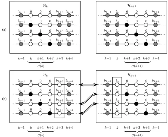
respec-tively. Let denote the set of the hypotheses con-sisting of the respective and (the latter is the same for all hypotheses). It can be shown—the case will be elaborated presently—that is invariant to a shift of the neighborhood to for a given if the nonoverlapping parts of and contain only zeros. (In that case, also the nonoverlapping parts of and contain only zeros.) This means that, if some is contained in both and and the nonoverlapping parts of and contain only zeros, the probability of this is the same in the sampling substeps corresponding to and ; thus, it has to be calculated only once.
An example for the case (corresponding to hypothesis sets and ) is shown in Fig. 1. It is assumed
that , so there are hypotheses in
and also in . In [see the left box in Fig. 1(a)], there is one hypothesis with all indicators in —i.e., —equal to zero. The other hypotheses each contain exactly one 1 in . The indicators at the
remaining positions, and , are
the same for all hypotheses. (Among them, note that , in particular, is equal to the respective realization drawn in the previous sampler iteration.)
Similarly, in [see the right box in Fig. 1(a)], there is one hypothesis with all indicators in —i.e.,
—equal to zero, and each of the other hypotheses contains exactly one 1 in . The remaining
indicators and are the same for
all hypotheses. (Among them, in particular, is equal to the respective realization drawn in the previous substep.)
The following can now be verified by inspection [see Fig. 1(b)]: If both drawn in the previous sampler iteration and drawn in substep [highlighted by boxes in Fig. 1(b)] are zero, then of the hypotheses in appeared already in . (In Fig. 1(b), these hy-potheses are indicated by arrows.) This means that only one
Fig. 1. (a) Hypothesis sets and for . White (black) nodes depict zero (nonzero) indicators. Gray nodes may be zero or nonzero, depending on the outcome of the past sampling substeps. (b) The same, under the condition that in (left set) and in (right set)—both are highlighted by boxes—are zero (white). It can be seen that sequences in also appear in , as indicated by the arrows.
hypothesis is new. Therefore, has to be
calculated only for one hypothesis; for all others, the values
of from the previous sampling substep
can be reused. (Note, however, that the values to be reused are those of (21), i.e., before normalization.)
Therefore, after sampling , (21) is calculated for only one hypothesis in substep (unless ), which amounts to an average computation of little more than one prob-ability per substep.3In the complementary case, i.e., after
sam-pling , we apply the first modification and skip
substeps. Then, we calculate (21) for hypotheses in the following substep . Again, this amounts to an average computation of approximately one probability per substep. The effects of the two modifications thus complement each other. When both modifications are used, the overall average com-plexity per PS iteration, , is reduced from about
to about , the number of substeps.
V. RESOLVING THESCALE ANDSHIFTAMBIGUITY A. Problem Formulation
Assuming for the moment an infinite temporal domain of ,
, and , we have for and
3The effect of the case on the overall complexity is small, since
is sparse and thus contains only few nonzero entries. This means that the case occurs very rarely.
, with an arbitrary amplitude scale factor and an arbitrary time shift . Provided that some
exists such that , this can be expressed
as toep toep . This equality has the following two consequences.
First, the observation is invariant to amplitude scalings and time shifts of the true and . Thus, unless the true parame-ters are constrained in a way that uniquely defines and , BD methods are inherently invariant to amplitude scalings and time shifts of the true and . This means that the BD result may feature an incorrect amplitude scale and time shift. In practice, this is not necessarily a major problem.
Second, the likelihood function in (13) is invariant to ampli-tude scalings and time shifts of its arguments:
toep
Therefore, the likelihood function is strongly multimodal: in-stead of a global maximum, there is an equivalence class of com-binations with different and that maximizes the likelihood. With respect to time shifts, however, the ambiguity is relaxed in our case because our system model does not satisfy the two assumptions made above, namely, infinite temporal sup-port and existence of a such that . In fact, since and are confined to the time intervals
of nonzero values or as they are shifted outside their re-spective interval. In this case, the likelihood changes. Further-more, a satisfying the time shift invariance relation
exactly typically does not exist; the relation can only
be satisfied approximately. This means that the likelihood func-tion is only approximately invariant to time shifts. Therefore, there is generally one specific time shift that fits the data best, although others may be almost as good.
As explained in Section II-C, our BD method is based on the joint posterior distribution
, where the likelihood appears as one of the factors. Due to the other factors, the pos-terior is not invariant to scalings and time shifts. Nevertheless, it usually preserves a multimodal structure similar to that of the likelihood function. This is problematic for both phases of MCMC detection/estimation: the generation of the sample and the sample-based detection/estimation.
B. Scale and Shift Ambiguity in the Sampling Phase
In the sampling phase, the multimodality of the posterior leads to slow convergence of the sampler. In fact, each has an “ideal partner” with respect to scale and shift, and vice versa. The sampling steps proposed in Section IV-B generate new realizations of and conditioned on the respective other vector, rather than jointly. Therefore, the scale and shift param-eters hardly change, i.e., the sampler stays within one mode of the likelihood for many iterations. Following [23], [48], this problem can be avoided by adding two joint sampling steps for , one for shift compensation and one for scale compen-sation. Both are inserted after the first PS step, i.e., after sampling (see Section IV-B), and they use the Metropolis–Hastings (MH) sampling algorithm [29, p. 267]. Based on the current realization , we first sample a proposal from
some proposal kernel . Then, with some
acceptance probability , we replace by ,
i.e., becomes the current realization of the sampler, whereas with probability , remains the current
realization. Here, is determined by and
the stationary distribution of the sampler, (see [29, p. 267] and [48] for details).
The first MH sampling step is for shift compensation and con-sists of the following substeps.
• Sample from a uniform distribution on , denoted , with some fixed . • Obtain and from and by means of a circular
shift by steps, i.e., and
.
• Sample from [see (19)]. (It can be
shown that this corresponds to the proposal kernel .)
• With probability , replace , , and by , , and , respectively. Here,
where with and
as defined in (20).
This shift compensation method differs from that in [23] and [48] by the support of the uniform distribution of , which is instead of { 1,0,1}. This allows larger jumps, which we observed to be beneficial. Another difference, due to our different priors, is the presence of in the expression of .
The MH sampling step for shift compensation is succeeded by that for scale compensation, which is based on the same con-cept and consists of the following substeps:
• Generate by sampling from
with some fixed and from a uniform distribution on . (These pdf’s will be denoted by and .)
• The proposal consists of , , and ,
where , , and denote the realizations that were accepted in the shift compensation step. (It can be shown that this corresponds to the proposal kernel
.)
• With probability , replace by and by . Here,
After shift/scale compensation, the PS continues with the sampling step, as described in Section IV-B.
C. Scale and Shift Ambiguity in the Detection/Estimation Phase
In the sample-based detection/estimation algorithms of Section III, the scale and shift ambiguity causes severe prob-lems. For example, the estimators are averages over the sample , which become mean-ingless if the individual realizations
feature different scales and shifts. A method for achieving identical scales and shifts in all realizations is described in [48].
VI. NUMERICALSTUDY A. Simulation Setup
We will compare the performance of the proposed sampling method (PS) with that of the AS described in Section IV-D. As a performance benchmark, we also consider the following “ref-erence sampler” (abbreviated RS) that does not exploit the min-imum-distance constraint.
One RS iteration
• Sample from .
• For , sample from .
• Sample from .
• Sample from .
This sampling algorithm, up to minor modifications, was pro-posed in [23] for a Bernoulli–Gaussian sequence . Note that
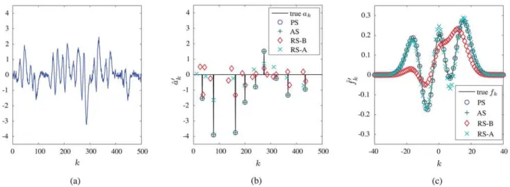
Fig. 2. Results of detection/estimation: (a) Signal , (b) estimates , (c) estimates . The results shown here are obtained after 60 iterations (PS and AS) or 1500 iterations (RS-A and RS-B). The vertical lines in (b) indicate the true . Real parts are shown.
our signal model is different because the Bernoulli–Gaussian prior of is modified by the minimum-distance constraint. Just as the PS and AS, the RS is a PCGS, not a classical Gibbs sam-pler, because the sampling distribution for is a conditional distribution associated with , rather than with the full joint posterior . The RS differs from the AS in that the AS exploits the minimum distance constraint by
sampling from . Like the AS, the RS
requires many matrix inversions. It is much more complex than the PS, even if the recursive inversion method of [23] is used.
We consider two versions of the RS. The first, denoted RS-A, is based on the true signal model (with minimum distance
con-straint), in which . Since the RS
be-haves like a classical Gibbs sampler with respect to dependen-cies within , it is not well suited to this prior. Therefore, we consider also a second RS version, denoted RS-B, which (at the cost of a model mismatch) is based on the unconstrained Bernoulli–Gaussian model for which the RS was proposed in [23]. We thus interpret realizations from as Bernoulli se-quences from , where is the approximation of described in Section II-B. It can be shown that the average distances between 1’s in sequences drawn from and are approximately identical. Consistently replacing
by and by in RS-A, we obtain RS-B.
We generated 100 realizations of from parameters ran-domly drawn according to the priors given in Section II-B,
using , , , , ,
, , , and (the latter two
parameters provide a noninformative prior for ). For each realization of , we generated four Markov chains according to the four sampler methods. Detection and estimation were then performed on each of the four samples as described in Section III. As mentioned in Section V, the time shift and amplitude scale of the estimate are arbitrary and, indeed, usually irrelevant. Therefore, for performance assessment, we matched the time shift and amplitude scale of each estimate to the true , i.e., we calculated the shifted/scaled version of
minimizing , and the corresponding shifted/scaled .
B. Simulation Results
As an example, the result of one simulation run—corre-sponding to one realization of —is shown in Fig. 2. Here, the detected/estimated sequences and pulse shapes of both the PS and AS are seen to coincide with the true and after only 60 iterations. The results of RS-A and RS-B after 1500 iterations are significantly worse. We note that all methods use the joint conditional estimator in (18); however, almost identical results are obtained with the componentwise sample-based estimator in (17).
To assess the convergence rates of the various samplers, Fig. 3(a) shows the empirical normalized mean-square error (NMSE) of versus the number of iterations. The empirical NMSE is defined as the average (over the 100 realizations) of normalized by the average of . The number of iterations indicated on the abscissa equals the total length of the Markov chain. Out of each chain, the last 20% of the iterations were used for detection/estimation. Again, was used for amplitude estimation; however, the NMSE obtained with is effectively equal for AS, RS-A, and RS-B and only about 0.3 dB higher for PS. The values of the NMSE of after 60 and 1500 iterations are also given in the first two rows of Table I. It is seen from Fig. 3(a) that RS-A fails to produce satisfactory results, and its error does not decrease with time. This is easily explained by the bad match between model and algorithm: the model features strongly dependent indicators because of the minimum distance constraint, whereas RS-A treats the indicators like a classical Gibbs sampler, which performs poorly in the presence of strong dependencies. This problem is circumvented in RS-B, since the model is adapted to the algorithm by dropping the minimum distance constraint. Indeed, we observe a steady decrease of the error, but at a very low rate: after 1500 iterations, the NMSE has only decreased by less than 2 dB. By contrast, both PS and AS achieve a low error after about 50 iterations. This fast convergence may appear surprising, as the MCMC concept is based on the law of large numbers. It can, however, be explained by the fact that the minimum distance constraint excludes large parts of the param-eter space that would otherwise have a nonnegligible posterior
Fig. 3. Detection/estimation performance versus the number of iterations: (a) Empirical NMSE of , (b) normalized average error of , (c) empirical NMSE of .
TABLE I
REPRESENTATIVESELECTION OFSIMULATIONRESULTS
probability. Within the remaining parts of the parameter space, the posterior probability is thus increased, which leads to faster convergence. From the superiority of the results of PS and AS over those of RS-A and RS-B, we can conclude that the use of the minimum distance constraint is highly beneficial.
In Fig. 3(b), we study the sparsity of the estimates (or, equivalently, ) by assessing the accuracy of . More specifically, we show the average (over the 100 realizations) of normalized by the average of versus the number of iterations. The values of the normalized average error of after 60 and 1500 iterations are also given in the third and fourth rows of Table I. In RS-B, the absence of a strict sparsity con-straint leads to very high values of (up to 5 times the true ) in the first iterations. After the first 10 iterations, the error slowly but steadily decreases. In RS-A, a certain level of spar-sity is enforced by the minimum distance constraint, leading to a normalized error between 0.07 and 0.09 after about 10 itera-tions. This error does not decrease with further iteraitera-tions. The sparsity achieved by RS-A may be meaningless in view of the failed convergence of . By contrast, both PS and AS reach er-rors below 0.04 after about 25 iterations.
Fig. 3(c) shows the empirical NMSE of versus the number of iterations. The results are roughly similar to those in Fig. 3(a). It can be seen that, in general, the error of the estimated pulse shapes is smaller than that of the estimated sparse sequences. Furthermore, RS-A outperforms RS-B because its realizations of are more sparse due to the minimum distance constraint. However, this is of little relevance since both RS-A and RS-B fail to estimate appropriately.
One reason why RS-B converges so slowly appears to be our choice of a relatively wide class of random pulse shapes in our simulation. To study this issue, we generated 100 realizations
Fig. 4. Empirical NMSE of versus the number of iterations, for realizations of using the pulse shape described in [23].
of from parameters drawn as described above, except that the pulse shape was fixed, namely, the one used in [23]. The estimation methods were not changed, i.e., they still estimated the pulse shape rather than using the true one. Fig. 4 shows the empirical NMSE of versus the number of iterations for this case. It is seen that the error of RS-B (and also that of PS and AS) decreases significantly faster than in Fig. 3(a). We can conclude that many of the pulse shapes that we generated randomly are harder to detect and estimate than the pulse shape used in [23].
Next, we illustrate the rationale of our choice of the block detector (see Section III-B). Out of a Markov chain of length 1000 generated by the PS, the last 200 realizations of were used as a sample. Within the sample, two realizations appear 22 times and no realization appears more than 22 times. In this case, the sample-based MAP sequence detector in
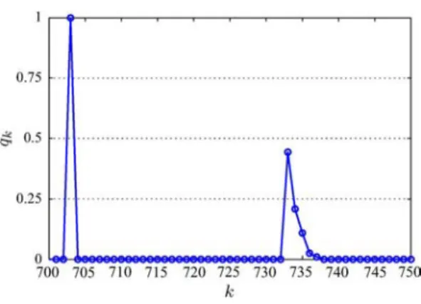
Fig. 5. Relative multiplicity versus .
Section III-A would fail, since the maximum is achieved by two realizations simultaneously. As explained in Section III-A, this is due to the coarse quantization of the probability. In another simulation run, again with sample size 200, we obtained a sequence that is depicted for in Fig. 5. Within that interval, there are two “zero intervals” (where no realization contains a 1, and thus in the zero intervals); these zero intervals are sep-arated by the “nonzero interval” (i.e.,
for all ). Within the sample, the following different realizations of occurred. Out of the 200 realizations, 89 contain a 1 at position 733, 42 contain a 1 at position 734, 22 contain a 1 at position 735, 4 contain a 1 at position 736, and 2 contain a 1 at position 737. The re-maining 41 realizations contain no 1 within . No realization contains more than one 1 within . Thus, at each position , less than half of the 200 realizations contain a 1; therefore, the component de-tector would not detect any 1’s. In the block dede-tector, on the other hand, the five positions are combined into a block . According to the multiplici-ties in the sample listed above, there are six hypotheses with relative multiplicities given by 89/200, 42/200, 22/200, 4/200, 2/200, and 41/200. The maximum relative multiplicity (89/200) is achieved by the hypothesis with a 1 at po-sition 733. Thus, the MAP block detector would detect a 1 at position 733, which is more intuitive than the result of the com-ponent detector.
We finally note that the computational complexities of the PS, AS, RS-A, and RS-B differ significantly. Exemplary computa-tion times for 20 iteracomputa-tions are reported in the last row of Table I for an unoptimized Matlab R2009b 64-bit implementation on a 2.2-GHz Intel Core 2 Duo processor. The processing time of the AS is almost 9 times that of the PS. This high complexity is not justified by a better performance, since (as shown by our simulation results) the performance of the AS is very similar to that of the PS. The processing times of the RS-A and RS-B are about 3 and 17 times that of the PS, respectively.
VII. CONCLUSION
We studied Bayesian blind deconvolution of an unknown sparse sequence convolved with an unknown pulse. Our ap-proach extended the conventional Bernoulli–Gaussian prior
(modeling sparsity) by a hard minimum distance constraint, which requires any two detected pulse locations to have a certain minimum separation. Such a constraint is physically motivated in many applications and is an effective means of avoiding spurious detected pulses. However, the minimum distance constraint implies strong dependencies, which lead to slow convergence of the classical Gibbs sampler. We demon-strated that this problem can be overcome by a new Monte Carlo blind deconvolution method based on the recently in-troduced PCGS principle. The proposed method exploits the structure that the constraint imposes on the parameter space to achieve fast convergence and low computational complexity. Our simulation results demonstrated a significant reduction of both the complexity and the number of spurious components compared to a recently proposed PCGS that is not specifically designed for the minimum distance constraint.
The proposed method can be easily generalized to inverse problems with a minimum distance constraint that are not de-scribed by a convolution model. This makes it potentially inter-esting for many signal processing applications including signal segmentation [49], optical coherence tomography [50], elec-tromyography [10], [11], and electrocardiography [13], [51]. Furthermore, the minimum distance constraint itself can be gen-eralized to a wider class of “local deterministic constraints,” which can be exploited in an analogous way [36].
APPENDIXA VALIDATION OF THEPS
To validate the PS as a PCGS, we will derive it from a clas-sical Gibbs sampler by means of marginalization and trimming (see [33] and Section IV-A). These modifications are allowed because they do not change the stationary distribution of the sampler. One iteration of the Gibbs sampler is given as follows:
• Sample from .
• For , sample from
.
• Sample from .
This is a valid Gibbs sampler, since each parameter is sampled once per iteration and each sampling distribution is conditioned on all other parameters (i.e., all except those being sampled).4
This concept is not compromised by the fact that some parame-ters are sampled jointly, namely and as well as all entries of .
The first modification we use is a marginalization, which leads to a sampler in which the second step of the Gibbs sampler is replaced by the following:
• For , sample from
.
Here, additional parameters are sampled in each sampling step. The sampler is no longer a Gibbs sampler, since the and (for all ) are now sampled several times within each sampler it-eration, in varying combinations. The choice of
as a replacement of the tuple sampled by the original Gibbs sampler is key to the fast convergence of the PS. On 4As mentioned in Section IV-B, does not appear in the conditions of the
sampling distributions of and because, for a given , is conditionally independent of and .
the one hand, the subvector is large enough so that the parameters that strongly depend on each other (due to the minimum distance constraint) are sampled jointly. On the other hand, it is small enough to allow efficient sampling as discussed below (22). Note that all sampling distributions are still conditioned on all parameters except those sampled. Thus, they are still conditionals associated with the joint posterior
.
Next, we apply trimming to obtain the following modified second step:
• For , sample from
.
Since some entries of —namely, all except —are removed from the argument of the sampling dis-tribution of the respective substeps, these sampling disdis-tributions are no longer proportional to the joint posterior . As previously explained in Section IV-B, the trimming is
justi-fied because all elements of except
itself are also contained in .
Therefore, out of , the untrimmed sampler uses only in the condition of the next substep, whereas the other entries are ignored. (This is true even for , trivially,
since .)
Finally, joint sampling of can be achieved by first sampling and then sampling conditioned on the thus obtained. Thus, the following final version of the second step is obtained:
• For ,
— sample from ;
— sample from .
Together with the first and third steps of the Gibbs sampler, this is equal to the PS described in Section IV-B.
APPENDIXB SAMPLINGDISTRIBUTIONS
In this appendix, we derive the sampling distributions used by the PS (cf. Section IV-C).
Pulse Coefficients: To obtain the sampling distribution for
in (19) and (20), we note that
We now insert (13) and (11), and obtain
This can be rewritten in terms of and as defined in (20):
Finally, normalization leads to ,
which equals (19).
Indicators: In order to derive (21) and (22), we start from
. Noting that is
composed of and and is composed of
and , and using (14), we obtain
In the last step, we used (7) and dropped factors that are constant with respect to and . Using (13) and again (7) yields
(26)
where and consists of the
columns of indexed by .
We now exploit the minimum distance constraint, i.e., the fact that can contain at most one nonzero entry. We will
con-sider the cases and separately. (This
means that we may not drop any constant factors until we find a joint expression for both cases.) For the case , let denote the (unknown) position of the nonzero entry. Noting that and using (8), we can write (26) as
Using and as defined in (22), this can be rewritten as
Integrating out then yields
(28)
For the case , we can rewrite (26) as
Integrating out gives
(29)
Now according to (22), implies that and
. Formally inserting these values into (28) yields (29).
Therefore, (28) is valid for both and .
Finally, dropping the constant factors in (28) yields (recall from (22) that and depend on )
which is (21).
Amplitudes: For the derivation of the distribution in (23), we
first note that
The right-hand side can be calculated by marginalizing with respect to all
entries of and except and : using to
denote , we have
(30) We will develop this expression separately for the two cases in (23), i.e., for and . For , the summation collapses:
(31) This is due to the minimum distance constraint: if , then the only hypothesis for with potentially nonzero
proba-bility is . Our case , is a special
case of , namely with . We now recall that
an expression of for the case
was given in (27). For , (27) reads
where constant factors have been dropped. Inserting this into (31) yields
or, equivalently,
. As explained below (24), due to , and equal, respectively, and as given in (24). Thus, we have verified (23) for .
In the complementary case , we can rewrite (26) as
Inserting this into (30) yields
After proper normalization, we obtain
, which is (23) for .
Noise Variance: To derive the sampling distribution for
Inserting (13) and (12), we obtain further
Normalization then leads to , which is (25).
REFERENCES
[1] D. N. Godard, “Self-recovering equalization and carrier tracking in two-dimensional data communication systems,” IEEE Trans.
Commun., vol. 28, pp. 331–344, Nov. 1980.
[2] J. R. Treichler and B. G. Agee, “A new approach to the multipath cor-rection of constant modulus signals,” IEEE Trans. Acoust., Speech,
Signal Process., vol. 31, pp. 1867–1875, Feb. 1983.
[3] G. Xu, H. Liu, L. Tong, and T. Kailath, “Least squares approach to blind channel identification,” IEEE Trans. Signal Process., vol. 43, pp. 2982–2993, Dec. 1995.
[4] E. Moulines, P. Duhamel, J.-F. Cardoso, and S. Mayrargue, “Subspace methods for the blind identification of multichannel FIR filters,” IEEE
Trans. Signal Process., vol. 43, pp. 516–525, Feb. 1995.
[5] A. M. Bronstein, M. M. Bronstein, and M. Zibulevsky, “Relative op-timization for blind deconvolution,” IEEE Trans. Signal Process., vol. 53, pp. 2018–2026, Jun. 2005.
[6] J. M. Mendel and J. Goutsias, “One-dimensional normal-incidence in-version: A solution procedure for band-limited and noisy data,” Proc.
IEEE, vol. 74, pp. 401–414, Mar. 1986.
[7] J. Idier and Y. Goussard, “Stack algorithm for recursive deconvolution of Bernoulli–Gaussian processes,” IEEE Trans. Geosci. Remote Sens., vol. 28, pp. 975–978, Sep. 1990.
[8] Q. Cheng, R. Chen, and T.-H. Li, “Simultaneous wavelet estimation and deconvolution of reflection seismic signals,” IEEE Trans. Geosci.
Remote Sens., vol. 34, pp. 377–384, Mar. 1996.
[9] O. Rosec, J.-M. Boucher, B. Nsiri, and T. Chonavel, “Blind marine seismic deconvolution using statistical MCMC methods,” IEEE J.
Ocean. Eng., vol. 8, pp. 502–414, Jul. 2003.
[10] D. Ge, E. Le Carpentier, and D. Farina, “Unsupervised Bayesian de-composition of multi-unit EMG recordings using Tabu search,” IEEE
Trans. Biomed. Eng., vol. 56, pp. 1–9, Dec. 2009.
[11] D. Ge, E. Le Carpentier, J. Idier, and D. Farina, “Spike sorting by sto-chastic simulation,” IEEE Trans. Neural Syst. Rehabil. Eng., vol. 19, pp. 249–259, Jun. 2011.
[12] G. Kail, C. Novak, B. Hofer, and F. Hlawatsch, “A blind Monte Carlo detection-estimation method for optical coherence tomography,” in
Proc. IEEE Int. Conf. Acoust., Speech, Signal Process. (ICASSP),
Taipei, Taiwan, Apr. 2009, pp. 493–496.
[13] C. Lin, C. Mailhes, and J.-Y. Tourneret, “P and T-wave delineation in ECG signals using a Bayesian approach and a partially collapsed Gibbs sampler,” IEEE Trans. Biomed. Eng., vol. 57, pp. 2840–2849, Dec. 2010.
[14] S. Bourguignon and H. Carfantan, “Spectral analysis of irregularly sampled data using a Bernoulli Gauss model with free frequencies,” in Proc. IEEE Int. Conf. Acoust., Speech, Signal Process. (ICASSP), Toulouse, France, May 2006, pp. 516–519.
[15] S. Bourguignon, H. Carfantan, and J. Idier, “A sparsity-based method for the estimation of spectral lines from irregularly sampled data,”
IEEE J. Sel. Topics Signal Process., vol. 1, pp. 575–585, Dec. 2007.
[16] M.-H. Chen and J. J. Deely, “Bayesian analysis for a constrained linear multiple regression problem for predicting the new crop of apples,” J.
Agricult. Biol. Environ. Stat., vol. 1, pp. 467–489, Dec. 1996.
[17] G. A. Rodriguez-Yam, R. A. Davis, and L. L. Scharf, “A Bayesian model and Gibbs sampler for hyperspectral imaging,” in Proc. IEEE
SAM, Washington, DC, Aug. 2002, pp. 105–109.
[18] S. Moussaoui, D. Brie, A. Mohammad-Djafari, and C. Carteret, “Separation of non-negative mixture of non-negative sources using a Bayesian approach and MCMC sampling,” IEEE Trans. Signal
Process., vol. 54, pp. 4133–4145, Nov. 2006.
[19] N. Dobigeon, S. Moussaoui, J.-Y. Tourneret, and C. Carteret, “Bayesian separation of spectral sources under non-negativity and full additivity constraints,” Signal Process., vol. 89, pp. 2657–2669, Dec. 2009.
[20] C. Févotte, B. Torrésani, L. Daudet, and S. J. Godsill, “Sparse linear regression with structured priors and application to denoising of mu-sical audio,” IEEE Trans. Audio, Speech, Lang. Process., vol. 16, pp. 174–185, Jan. 2008.
[21] T. Blumensath and M. E. Davies, “Monte-Carlo methods for adaptive sparse approximations of time-series,” IEEE Trans. Signal Process., vol. 55, pp. 4474–4486, Sep. 2007.
[22] M. Ting, R. Raich, and A. O. Hero, “Sparse image reconstruction for molecular imaging,” IEEE Trans. Image Process., vol. 18, pp. 1215–1227, Jun. 2009.
[23] D. Ge, J. Idier, and E. Le Carpentier, “Enhanced sampling schemes for MCMC based blind Bernoulli–Gaussian deconvolution,” Signal
Process., vol. 91, pp. 759–772, Apr. 2011.
[24] M. Lavielle, “Bayesian deconvolution of Bernoulli–Gaussian pro-cesses,” Signal Process., vol. 33, pp. 67–79, Jul. 1993.
[25] F. Champagnat, Y. Goussard, and J. Idier, “Unsupervised deconvo-lution of sparse spike trains using stochastic approximation,” IEEE
Trans. Signal Process., vol. 44, pp. 2988–2998, Dec. 1996.
[26] A. Doucet and P. Duvaut, “Bayesian estimation of state-space models applied to deconvolution of Bernoulli–Gaussian processes,” Signal
Process., vol. 57, pp. 147–161, March 1997.
[27] K. Hausmair, K. Witrisal, P. Meissner, C. Steiner, and G. Kail, “SAGE algorithm for UWB channel parameter estimation,” presented at the COST 2100 Management Committee Meeting, Athens, Greece, Feb. 2010.
[28] G. Kail, K. Witrisal, and F. Hlawatsch, “Direction-resolved estimation of multipath parameters for UWB channels: A partially collapsed Gibbs sampler method,” in Proc. IEEE Int. Conf. Acoust., Speech,
Signal Process. (ICASSP), Prague, Czech Republic, May 2011, pp.
3484–3487.
[29] C. P. Robert and G. Casella, Monte Carlo Statistical Methods. New York: Springer, 2004.
[30] Markov Chain Monte Carlo in Practice, W. R. Gilks, S. Richardson, and D. J. Spiegelhalter, Eds. London, U.K.: Chapman & Hall, 1996. [31] S. Yildirim, A. T. Cemgil, and A. B. Ertüzün, “A hybrid method for deconvolution of Bernoulli–Gaussian processes,” in Proc. IEEE Int.
Conf. Acoust., Speech, Signal Process. (ICASSP), Taipei, Taiwan, Apr.
2009, pp. 3417–3420.
[32] S. Bourguignon and H. Carfantan, “Bernoulli–Gaussian spectral anal-ysis of unevenly spaced astrophysical data,” in Proc. IEEE SSP, Bor-deaux, France, Jul. 2005, pp. 811–816.
[33] D. A. van Dyk and T. Park, “Partially collapsed Gibbs samplers: Theory and methods,” J. Amer. Statist. Assoc., vol. 103, pp. 790–796, Jun. 2008.
[34] T. Park and D. A. van Dyk, “Partially collapsed Gibbs samplers: Il-lustrations and applications,” J. Comput. Graph. Statist., vol. 18, pp. 283–305, Jun. 2009.
[35] N. Dobigeon and J.-Y. Tourneret, “Bayesian orthogonal component analysis for sparse representation,” IEEE Trans. Signal Process., vol. 58, pp. 2675–2685, May 2010.
[36] G. Kail, J.-Y. Tourneret, F. Hlawatsch, and N. Dobigeon, “A partially collapsed Gibbs sampler for parameters with local constraints,” in
Proc. IEEE Int. Conf. Acoust., Speech, Signal Process. (ICASSP),
Dallas, TX, Mar. 2010, pp. 3886–3889.
[37] J. J. Kormylo and J. M. Mendel, “Maximum likelihood detection and estimation of Bernoulli–Gaussian processes,” IEEE Trans. Inf. Theory, vol. IT-28, pp. 482–488, May 1982.
[38] R. Haas and J.-C. Belfiore, “A time-frequency well-localized pulse for multiple carrier transmission,” Wireless Personal Commun., vol. 5, pp. 1–18, 1997.
[39] L. Sörnmo, P. Börjesson, M. Nygards, and O. Pahlm, “A method for evaluation of QRS shape features using a mathematical model for the ECG,” IEEE Trans. Biomed. Eng., vol. 28, no. 10, pp. 713–717, 1981. [40] A. J. E. M. Janssen, “Positivity and spread of bilinear time-frequency distributions,” in The Wigner Distribution—Theory and Applications
in Signal Processing, W. Mecklenbräuker and F. Hlawatsch, Eds.
Amsterdam, The Netherlands: Elsevier, 1997, pp. 1–58.
[41] F. Hlawatsch, Time-Frequency Analysis and Synthesis of Linear Signal
Spaces: Time-Frequency Filters, Signal Detection and Estimation, and Range-Doppler Estimation. Boston, MA: Kluwer, 1998.
[42] C. P. Robert, The Bayesian Choice. New York: Springer, 1996. [43] N. Dobigeon, J.-Y. Tourneret, and J. D. Scargle, “Joint segmentation of
multivariate Poissonian time series. Applications to burst and transient source experiments,” in Proc. EUSIPCO, Florence, Italy, Sep. 2006. [44] S. M. Kay, Fundamentals of Statistical Signal Processing: Detection