HAL Id: hal-01004987
https://hal.archives-ouvertes.fr/hal-01004987
Submitted on 2 Feb 2017
HAL is a multi-disciplinary open access
archive for the deposit and dissemination of
sci-entific research documents, whether they are
pub-lished or not. The documents may come from
teaching and research institutions in France or
abroad, or from public or private research centers.
L’archive ouverte pluridisciplinaire HAL, est
destinée au dépôt et à la diffusion de documents
scientifiques de niveau recherche, publiés ou non,
émanant des établissements d’enseignement et de
recherche français ou étrangers, des laboratoires
publics ou privés.
Distributed under a Creative Commons Attribution| 4.0 International License
Elastoplastic Model for Clay with Microstructural
Consideration
Ching S. Chang, Pierre Yves Hicher, Z.Y. Yin, L.R. Kong
To cite this version:
Ching S. Chang, Pierre Yves Hicher, Z.Y. Yin, L.R. Kong. Elastoplastic Model for Clay with
Mi-crostructural Consideration. Journal of Engineering Mechanics - ASCE, American Society of Civil
Engineers, 2005, 42 (14), pp.4258-4277. �10.1061/(ASCE)EM.1943-7889.0000013�. �hal-01004987�
Elastoplastic Model for Clay
with Microstructural Consideration
C. S. Chang
1; P.-Y. Hicher
2; Z. Y. Yin
3; and L. R. Kong
4Abstract:Clay material can be considered as a collection of clusters, which interact with each other mainly through mechanical forces. From this point of view, clay is modeled by analogy to granular material in this paper. An elastoplastic stress-strain relationship for clay is derived by using the granular mechanics approach developed in previous studies for sand. However, unlike sand, clay deformation is generated not only by the mobilizing but also by compressing clusters. Thus, in addition to the Mohr-Coulomb’s plastic shear sliding and a dilatancy type flow rule, a plastic normal deformation has been modeled for two clusters in compression. The overall stress-strain relationship can then be obtained from the mobilization and compressing of clusters through a static hypothesis of the macro-micro relations. The predictions are compared with the experimental results for clay under both drained and undrained triaxial loading condi-tions. Three different types of clay, including remolded and natural clay, have been selected to evaluate the model’s performance. The comparisons verify that this model is capable of accurately reproducing the overall behavior of clay, which accounts for the influence of key parameters such as void ratio and mean stress. A section of this paper is devoted to show the model’s capability of considering the influence of inherent anisotropy on the stress-strain response under undrained triaxial loading conditions.
keywords: Clays; Microstructures; Stress strain relations; Anisotropy; Elastoplasticity.
Introduction
Under a microstructural approach for stress-strain modeling, a set of microsystems共e.g., interparticle contacts兲 is used to represent the material. Material properties are defined for each microsystem and the overall stress-strain relationship for the material is ob-tained from averaging the behaviors of this set of microsystems. If the microsystems are considered as a set of mobilized planes in the material, the approach used to estimate the overall behavior from this set of planes can be linked to G. I. Taylor’s concept, developed long ago, as the slip theory of plasticity for polycrys-talline materials by Batdorf and Budianski 共1949兲. These ideas were applied by Pande and Sharma 共1982兲 to rocks and soils in what they called the overlay model, and to concrete by Bazant et al.共1996兲 in the so-called microplane model.
For granular material, a set of particle pairs in contact are considered as the microsystems, and material constants are de-fined for the interparticle contacts. The approach used to estimate
the overall stress-strain behavior of granular material can be found in the work done over the last two decades. For elastic behavior, work has been done by Jenkins共1988兲, Walton 共1987兲, Rothenburg and Selvadurai共1981兲, Chang 共1988兲, Emeriault and Cambou 共1996兲, Liao et al. 共2000兲, and Kruyt and Rothenburg 共2002兲, among others. For inelastic stress-strain behavior, models can be found in Jenkins and Strack共1993兲, Matsuoka and Takeda 共1980兲, Chang et al. 共1989a,b兲, etc. Chang et al. 共1992a,b兲, and Suiker and Chang 共2004兲. These inelastic models have encoun-tered some difficulties in predicting the correct shear strength in so far as the predicted strength is often overestimated for the models with a kinematic hypothesis 共Chang and Misra 1990兲. These models also have difficulties in predicting correctly the behavior under different stress paths. To overcome these difficul-ties, we have adopted a static hypothesis proposed by Liao et al. 共1997兲 and incorporated the critical state concept to formulate a microstructural model suitable for sand共Chang and Hicher 2005兲. In this paper, we treat clay as a collection of clusters formed by groups of platy clay particles. At the scale of cluster sizes, long range forces are negligible, and the clusters interact with each other mainly through mechanical forces. Thus, clay material can be modeled by analogy to granular material. Some studies on clay fabric supporting this notion are discussed in the “Simple Model for Clay Fabric” section. A stress-strain model is then presented in the “Stress-Strain Model” section, in which we consider a clay cluster as a deformable grain. We then extend the granular me-chanics approach 共i.e., Chang and Liao 1990; Chang and Gao 1995; Chang and Hicher 2005兲 to derive the elastoplastic stress-strain relationship for clay.
The model’s performance is then evaluated by comparing the predicted with the measured triaxial loading results for clay speci-mens of various overconsolidation ratios 共OCRs兲, under various confining stresses, and in both drained and undrained conditions. The experimental results are obtained from two types of remolded
1Professor, Dept. of Civil and Environmental Engineering, Univ. of
Massachusetts, Amherst, MA 01003 共corresponding author兲. E-mail: [email protected]
2Professor, Research Institute in Civil and Mechanical Engineering,
UMR CNRS 6183, Ecole Centrale Nantes, BP 92101, 44321 Nantes, France.
3
Visiting Researcher, Univ. of Massachusetts, Amherst, MA 01003.
4Research Assistant, Research Institute in Civil and Mechanical
Engineering, UMR CNRS 6183, Ecole Centrale Nantes, BP 92101, 44321 Nantes, France.
clay with very different compressibilities. A natural clay with in-herent anisotropy has also been studied to evaluate the model’s ability to model the effects of inherent anisotropy on the stress-strain response under undrained triaxial loading condition.
Simple Model for Clay Fabric
The constituents of clay can be generally viewed across three scales
1. Clay particle: a clay particle is usually platy in shape. Its thickness and size can vary 100 times according to specific clay types, such as montmorillonite, illite, or kaolinite. The size for a platy particle generally ranges from 0.01– 1 m. 2. Clay cluster as an aggregate of clay particles: clay particles
attract each other due to surface forces among particles such as chemical, electrostatic, van der Waals forces, etc. These forces pull together the particles to form particle clusters, which have either a flocculate or dispersed type structure, as shown in Fig. 1. The size of the clusters continues to grow until the clusters are large enough so that the cluster weight, due to gravitation, becomes significantly larger than the in-terparticle surface forces. At this stage, the cluster loses its potential to attract further clay particles, and the size of clus-ters stops to grow. The ultimate cluster-size depends on the clay particle type, the liquid inside the pores, and its sedi-mentation history.
3. Clay material as an assembly of clusters.
Since the clay-particles are strongly attracted to each other by surface forces, a cluster of particles does not deform very much under usual external stresses and can, therefore, be considered as an intact unit. On the other hand, clusters interact mainly through mechanical forces. Thus, as schematically shown on the left side of Fig. 2, clay can be regarded as an assembly of “grains,” in which each grain is also a cluster. The main difference between sand grains and clay clusters is that the clay clusters, compared to sand grains, are more deformable. This deformability depends on the way the clay particles are assembled, which is a function of the mineralogy, adsorbed ions, etc.
A study undertaken by Hicher et al.共2000兲, by means of scan-ning and transmission electron microscopes, related the mechani-cal behavior of two saturated remolded clays, a kaolinite and a bentonite, to the evolution of their microstructural parameters such as particle shape, particle size, and particle orientation. The results of this study show that the main role played by the clay clusters is similar to the role played by the grains in the mechani-cal behavior of granular materials. This explains why sand and clay have similar qualitative behavior even though each material consists of different constituents 共Biarez and Hicher 1994兲. The difference in nature between sand grains and clay clusters can nevertheless explain quantitative differences in their stress-strain relationship. In particular, the deformability of the clusters can have a significant effect on volume change behavior in drained condition and on the shape of stress path in undrained condition. The influence of the cluster’s deformability on the elastic proper-ties of clayey materials is particularly pronounced. Since the elas-tic domain is restricted to very small strains共⬍10−5兲, for which the relative displacements of the clusters are negligible, the de-formation of the material must be mainly due to the dede-formation of individual clusters. Thus, the elastic moduli measured in sands and gravels are much higher than those in clays 共Biarez and Hicher 2008兲.
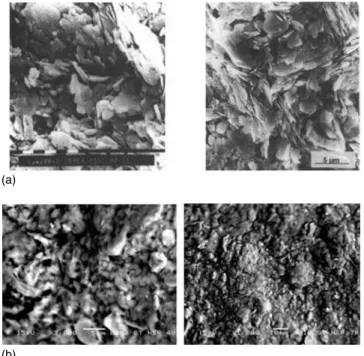
At higher strain level, the major deformation mechanism of the continuous medium is due to the relative displacements of the clay clusters. Under theses conditions, the main factor affecting the overall behavior is the friction between clusters, determined by the nature and the shape of these clusters. The photographs in Fig. 3共a兲 show how kaolinite microstructure is made up of rigid small particles and aggregated in compact clusters. Fig. 3共b兲 shows the clusters of both natural and remolded Saint Herblain clay.
An analysis of the pore size distribution in the kaolinite, by means of mercury intrusion porosimetry, confirmed the existence of two major groups of pore sizes: one centered around 1 m
Flocculate
Disperse
Fig. 1.Flocculate and disperse structure of clay particles
Fig. 2.Schematic illustration of clay clusters as grains
(b) (a)
Fig. 3. 共a兲 Microstructure of a kaolinite clay: left photo: isotropic
consolidation= 10 kPa and right photo: isotropic consolidation = 300 kPa;共b兲 microstructure of Saint Herblain clay: left photo: natu-ral clay共5 m兲 and right photo: remolded clay 共10 m兲
and the other around 10 nm. The first group corresponds to the intercluster pores, whereas the second one is related to the inter-particle pores. The number and the size of large pores progres-sively decreased wit increasing consolidation stresses, while the small pore size remained relatively unchanged under moderate loading stresses. This result confirmed that the volume change during loading is mainly due to the rearrangement of the clay-clusters共Hicher et al. 2000兲.
Stress-Strain Model
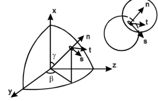
In this model, clay is regarded as an aggregate of clusters. The deformation of a representative volume of the material is gener-ated by mobilizing and compressing the clusters. Thus, the stress-strain relationship can be derived as an average of the deformation behavior of local contact planes in all orientations. For contact planes in the ␣th orientation, the local forces f␣j and the local movements ␦i␣ are denoted by fj␣=兵fn␣, fs␣, ft␣其 and
␦i␣=兵␦n␣, ␦s␣, ␦t␣其, where the subscripts n, s, and t represent the
components in the three directions of the local coordinate system, as shown in Fig. 4. The direction outward normal to the plane is denoted as n; the other two orthogonal directions, s and t, are tangential to the plane.
Density State of a Cluster Assembly
One of the important elements to consider in soil modeling is the critical state concept. At critical state, the clay material remains at a constant volume while it is subjected to a continuous distortion. The void ratio corresponding to this state is ec.
The critical void ratio ec is a function of the mean stress
p =共x+y+z兲/3. The relationship has traditionally been written
as follows:
ec= ecr0− ln
冉
p
pcr0
冊
共1兲 The two parameters 共ecr0, pcr0兲 represent a reference point on the critical state line. For convenience, the value of pcr0is taken to be 0.01 MPa. The critical state line can be defined by two param-eters ecr0and. Using the critical state concept, the density state of an assembly is defined as the ratio e/ec, where e is the void
ratio of the assembly.
Intercluster Behavior
In order to have a more apparent link between the micro and macro variables, we define a local stressi␣and a local strain␥i␣, which are directly related to the local forces f␣j and the local movements␦i␣at each contact by
i␣= Nl␣ 3Vfi ␣; ␥ i ␣=␦ i ␣/l␣ 共2兲
where l␣= length of the branch vector, which joins the centroids of two contact clusters, and V = volume of the representative ele-ment. It is to be noted that the local stressi␣is not the stress on the physical contact area between two clusters. It should be viewed rather as the average stress on the intercluster plane when the cluster and voids in the representative volume are homog-enized into a continuum. For an isotropic medium, the local stress is identical to the tractions resolved on the plane due to global stress共i.e., i␣=jin␣j兲. The proof will be given later in Eq. 共19兲.
In the local coordinate system, the local stress and local strain are respectively denoted as 兵n␣ s␣ t␣其 and 兵␥n␣ ␥s␣ ␥t␣其. For convenience, we use the notation␣=n␣for local normal stress and the notation ␣=␥n␣for local normal strain in the following sections.
Elastic Part
The intercluster behavior can be characterized as the relationship between contact force and contact displacement, given by
fi␣= kij␣␦␣j 共3兲
in which the stiffness tensor can be related to the contact normal stiffness, kn␣, and shear stiffness, kr␣
kij␣= kn␣ni␣n␣j+ k␣r共si␣s␣j+ ti␣tj␣兲 共4兲
In terms of local stress and local strain, an alternative intercluster stiffness is defined as i␣= k¯ij␣␥j␣ 共5兲 where k ¯ ij ␣= k ij ␣N共l␣兲2 3V 共6兲
The intercluster stiffness can be expressed as the form adopted for sand grains by Chang et al.共1989a,b兲, given by
k ¯ n ␣= k¯ n0 ␣
冉
␣ pref冊
n ; ¯kr␣= krR¯kn␣= krR¯kn0␣冉
␣ pref冊
n 共7兲 where␣= local stress in a normal direction; pref= standardrefer-ence pressure taken as 1 MPa.; and krR= ratio of shear to normal
stiffness. k¯n0␣, krRand n are material constants. The value of n is
found to be 0.33 for two elastic spheres according to Hertz-Mindlin’s formulation 共Mindlin 1969兲. Based on experimental measurements of the elastic modulus under different confining stress, the value of n has been found to be 0.5 for sand and 0.5–1.0 for clay.
Plastic Part
Shear Sliding
The elastic part of the tangential movement between two clusters does not have a coupling effect 共i.e., there is no shear induced normal movements兲. However, plastic sliding often occurs along the tangential direction of the contact plane with an upward or downward movement 共i.e., dilation or contraction兲. Stress dila-tancy is a well-known phenomenon in sand关see discussions in the work by Taylor共1948兲, Rowe 共1962兲, Goddard 共1990兲, etc.兴, and should be correctly modeled. The dilatancy equation used here is modified from the equation adopted for sand by Chang and Hicher共2005兲, given by dp d␥p=共sgn兲b
冉
− tan冊冉
冊
a冉
1 − e ec冊
共8兲 The modified equation allows more flexibility in modeling per-formance for different behaviors. In this equation, a, b, and are intercluster property constants, ecis the critical void ratio forthe clay, and 共sgn兲 is the sign of 共/−tan 兲. When the void ratio e is equal to the critical void ratio, zero dilation holds. It is to be noted that the state variables e and ecof the clay are referred
to the cluster assembly, which is used to regulate the dilation of individual intercluster contacts. It is rational to consider the micro variable as a function of the macrostate because the intercluster behavior is indeed influenced by the density state of the specimen. In Eq.共7兲, is the intercluster friction angle, which, in value, is very close to the internal friction angle, measured at critical state. The values of a and b can be calibrated from experimental measurements of triaxial tests, which will be shown in the later section on numerical simulation.
Note that the shear stress and the rate of the plastic shear strain d␥pin Eq.共7兲 are defined as
=
冑
s2+
t
2 and d␥p=
冑
共d␥sp兲2+共d␥tp兲2 共9兲
The yield function is assumed to be of Mohr-Coulomb type, given by
F1共,,1兲 = − 1共␥p兲 = 0 共10兲 where 1共␥P兲=isotropic hardening/softening parameter. Plastic loading corresponds to dF1⬎0. The hardening parameter is defined by a hyperbolic function in the 1-␥p plane, which in-volves two material constants: pand k¯p through the following
relationship: 1= k ¯ ptanp␥p tan p+ k¯p␥p 共11兲 When plastic deformation increases, 1 asymptotically ap-proaches tanp. For a given value of, the initial slope of the
hyperbolic curve is k¯p/. The flow rule is nonassociated. Under a
loading condition, the shear plastic flow in the direction tangential to the contact plane is determined by a normality rule applied to the yield function. However, the plastic flow in the direction nor-mal to the contact plane is governed by the stress-dilatancy equa-tion in Eq.共7兲.
The value of k¯pis found to be linearly proportional to k¯nsuch
that k ¯ p ␣= k pR¯kn␣= kpR¯kn0␣
冉
␣ pref冊
n 共12兲 The ratio kpRis a material parameter.The internal friction angle is a constant for a given mate-rial. However, the apparent friction angle,p, on a contact plane
is dependent on the density state of neighboring clusters, which can be related to the void ratio e by
tanp=
冉
ec
e
冊
m
tan 共13兲
where m = material constant共Biarez and Hicher 1994兲.
In a loose structure, clusters can rotate more freely, preventing the intercluster shear force from fully mobilizing the sliding re-sistance. The apparent frictional anglepis smaller than. On
the other hand, a dense structure has a higher degree of interlock-ing, which requires more effort to mobilize the contacts between clusters. In such a case, the apparent frictional anglepis greater
than . When the loading stress reaches the apparent frictional anglep, the dense structure dilates and the degree of
interlock-ing becomes relaxed. As a consequence, the apparent frictional angle共i.e., the peak angle in this case兲 is reduced, which results in a strain-softening phenomenon.
Normal Compression
To describe the compressible behavior between two clay clusters, a second yield surface is necessary. The second yield function is assumed to be as follows:
F2共,2兲 = − 2共p兲 for ⬎ p
p 共14兲
where the local normal stress and local normal strain p are
defined in Eq.共3兲. The hardening function 2共p兲 is defined as 2=p10 p/c p or p= c plog 2 p 共15兲 where cp= compression index for the compression curve plotted
on thep− log plane. When is less than
p, the plastic strain
produced by the second yield function is null. Thus, p in
Eq. 共12兲 corresponds to the preconsolidation stress in soil mechanics.
Elastoplastic Relationship
With the basic elements of intercluster behavior共elastic and plas-tic兲 discussed above, the final incremental local stress-strain rela-tion of the intercluster contact can be derived
˙i␣= k¯ij␣p␥˙␣j 共16兲
Since it is a standard procedure to derive a detailed expression for the elastoplastic stiffness tensor k¯ij␣p by using the plastic yield functions given above, the derivation is not presented here.
Stress-Strain Relationship
The stress-strain equations at cluster scale represent the relation-ships between two vectors—intercluster stress iand intercluster
strain ␥j—whereas the stress-strain equations at the assembly
scale represent the relationships between two tensors—stressij
and strainkl. Due to the two different levels of complexity, it is
stress-strain equations at cluster scale than those at assembly scale. Thus, in the present model, the stress-strain equations at cluster scale are first established in a phenomenological manner, as shown in the last section. In this section, these equations are used to derive the stress-strain equations at assembly scale. This way is more rational and takes less effort than a straight phenom-enological approach of establishing the stress-strain relationship at assembly scale.
Macro-Micro Relationship
The stress-strain relationship for an assembly of clay clusters can be determined from integrating the intercluster behavior at all contacts. During the integration process, a relationship is required to link the macro and micro variables. Using the static hypothesis proposed by Liao et al.共1997兲, we obtain the relation between the strain of assembly and intercluster strain
u˙j,i=
兺
␣=1 N
␥˙␣jnk␣Bik␣ 共17兲
where␥˙j= local strain between two contact clusters; nk= unit
vec-tor of the branch joining the centers of two contact clusters; and N = total number of contacts, over which the summation is carried out. The tensor Bik␣ in Eq.共16兲 is defined as
Bik␣= Aik−1共l␣兲2 where the fabric tensor Aik=
兺
␣=1 Nli␣lk␣ 共18兲
Using the principle of energy balance, which states that the work done in a representative volume element is equal to the work done on all intercluster planes within the element, we have
iju˙j,i= 1 V
兺
␣=1 N fj␣␦˙␣j= 3 N兺
␣=1 N j␣␥˙␣j 共19兲and using Eq. 共16兲, the local stress on the ␣th contact plane is derived as follows: ˙␣j= N 3˙ijBik ␣n k ␣ 共20兲
For the case of isotropic fabric, it can be derived that Bik
= 3␦ik/N, where ␦ik is the Kronecker delta. Thus Eq. 共19兲 is
re-duced to the usual form˙␣j=˙ijn␣j.
The stress increment˙ijcan be obtained by adding the dyadic
product of the contact force and the branch vectors for all contacts 共Christofferson et al. 1981; Rothenburg and Selvadurai 1981兲. In terms of local stress, it is
˙ij= 1 V
兺
␣=1 N fj␣li␣= 3 N兺
␣=1 N ␣jni␣ 共21兲Applying the defined local stress in Eq.共19兲, Eq. 共20兲 is uncon-ditionally satisfied.
By using Eqs.共15兲, 共16兲, and 共19兲, the following relationship between stress and strain can be obtained:
u˙i,j= Cijmp˙mp 共22兲
where Cijmp= N 3
兺
␣=1 N 共k¯jp ep兲−1n k ␣n n ␣B ik ␣B mn ␣ 共23兲The summation in Eq. 共22兲 can be expressed by a closed-form solution for some limited conditions such as the elastic modulus of randomly packed equal-size particles 共Chang et al. 1995兲. However, for elastic-plastic behavior, due to the nonlinear nature of the local constitutive equation, a numerical calculation with an iterative process is needed to carry out the summation in Eq.共22兲.
Computation Scheme
Initially, we know the global variables共ijandij兲 for the
assem-bly and the local variables 共f␣j and␦j␣兲 for each contact. For a given loading increment, which can be of a stress control, a strain control or a mixed mode, 6 out of the 12 variables共⌬ijand⌬ij兲
are unknown. The objective is to determine all global共ijandij兲
and local variables 共f␣j and␦␣j兲 at the end of the load increment. For a system with N intercluster contacts, the number of un-knowns is 3N for fj␣ and 3N for ␦j␣. The total number of un-knowns is therefore 3N + 3N + 6.
The following constraints must be satisfied:
1. The local constitutive equation, i.e., Eq.共15兲. Since there are three equations for each contact, the total number of equa-tions is 3N; N being the total number of intercluster contacts. 2. The static hypothesis between global stress and local forces,
i.e., Eq.共19兲: the number of equations is 3N.
3. The strain definition between global strain and local dis-placement, i.e., Eq.共16兲. The number of equations is 6 共strain tensor is symmetric兲.
The total number of unknowns is the same as the total number of equations. Therefore, a solution can be determined. To facili-tate the numerical calculation, the summation process in the above equations can be replaced by an integral process in a spherical coordinate system with an orientation distribution func-tion E共␣,兲 for the intercluster contacts, provided that the num-ber of contact N is sufficiently large共Chang and Misra 1990兲. An example is the fabric tensor in Eq.共17兲
Aik=
兺
␣=1 N li␣lk␣= N 2冕
0 /2冕
0 2 E共␣,兲li共␥,兲lk共␥,兲sin ␥d␥dThe surface integration on a sphere can be carried out numeri-cally through Gaussian integration points with weight factors. Thus the integration process requires less effort than the summa-tion process because it can be integrated over a small number of Gaussian integration points共i.e., selected number of contact ori-entations兲. Lebedev 共1976, 1977兲 has pioneered an integration scheme using a set of integration points with octahedral symme-try. Bazant and Oh 共1986兲 has devised an integration method similar to the ones proposed by Lebedev. Along this line, a more refined method has been proposed by Delley共1996兲 for applica-tions in weather forecasting, quantum chemistry, wave scattering, and radiation studies.
For all simulations presented in this paper, we have performed using three numbers of integration points N = 56, N = 74, and N = 122. The predicted stress-strain curves show about 5–7% dif-ference between the results obtained from integration numbers N = 56 and 74, whereas the curves show less than 1% difference between the results obtained from integration numbers N = 74 and 122. Thus N = 74 was found to be adequate. However, it is
antici-pated that in the case of strong anisotropy, the number of orien-tations may require higher values to reach convergence.
For a strain-controlled test, Eq.共21兲 presents numerical diffi-culties at the after-peak range with strain softening. In this case, a method of “elastic predictor-plastic corrector” was adopted to ob-tain the solution. The most widely used method for the solution of nonlinear constitutive equations is in the category of elastic predictor-plastic corrector method 共Ortiz et al. 1983兲, where a purely elastic trial state is followed by a plastic corrector stage 共return mapping algorithm兲. The purpose of the return mapping is to enforce consistency, at the end of the load step, of the pre-scribed yield surface and flow rule. For simple classical plasticity models, the return path can be determined in closed form. How-ever, for the present model that accounts for pressure sensitive nonlinear work hardening/softening, nonlinear elasticity, and two yield surfaces, it becomes necessary to compute the return path in an iterative fashion. An implicit integration scheme is more stable to obtain the solution of the system of nonlinear equations through iterative processes. The specific method adopted for com-putation is the single step backward Euler return method 关see Simo and Hughes共1998兲兴.
It is to be noted that the implicit integration scheme with the single step backward Euler return method is applicable only for a strain controlled test. For a mix-mode loading condition共i.e., for some components, stresses are specified rather than strains such as that in triaxial compression test conditions兲, an additional it-eration process is also needed to satisfy the condition of specified
stresses. Since the procedure is straightforward, thus it is not in-cluded here.
Summary of Parameters
The material parameters are summarized as follows: 1. Microstructural descriptions共two parameters兲.
a. Contact number per unit volume, N/V and mean cluster size, d.
2. Intercluster properties共nine parameters兲.
a. Intercluster elastic constants: k¯n0, krR, and n.
b. Intercluster friction angle: and m.
c. Intercluster plastic normal compression index and plas-tic shear stiffness ratio: cpand kpR.
d. Dilation constants: a and b.
3. Density state of the assembly共three parameters兲. a. Critical state for the soil: and ecr0.
b. Reference void ratio, e0, on the isotropic compression line at p = 0.01 MPa.
The size of a clay cluster d can be estimated from looking at a photograph provided by a scanning electron microscope. The value of N/V is not easy to obtain directly from experiments on clay. According to the experimental data by Oda共1977兲 for three mixtures of spheres, the contact number per unit volume can be approximately related to the void ratio by
N V= 12 d3共1 + e兲e 共24兲 0 0.2 0.4 0.6 0.8 1 1.2 0 0.1 0.2 0.3 ε1 q (MP a) Experiment Simulation (a) NC pi= 0.4 MPa NC pi= 0.8 MPa 0 0.2 0.4 0.6 0.8 1 1.2 0 0.2 0.4 0.6 0.8 1 1.2 p' (Mpa) q( M P a) Experiment Simulation (b) NC pi= 0.4 MPa NC pi= 0.8 MPa 1 0.87 0.4 0.5 0.6 0.7 0 0.1 0.2 0.3 ε1 e Experiment Simulation (c) NC pi= 0.4 MPa NC pi= 0.8 MPa 0.4 0.5 0.6 0.7 0.01 0.1 1 10 p' (MPa) e (d) pi= 0.8 Isotropic consolidation
Critical state line
pi= 0.4
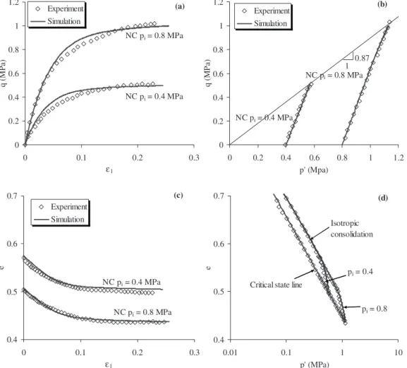
Fig. 5.Comparison of predicted results and experimental results for white kaolinite clay in drained tests:共a兲 stress-strain curves; 共b兲 effective stress paths;共c兲 void ratio versus axial strain curves; and 共d兲 void ratio versus mean stress curves
Here we use this equation as a first-order approximation to estimate N/V for clay by treating d as the mean size of the clay clusters. It is to be noted that the value of contact number per unit volume changes with void ratio. The evolution during the defor-mation process is taken into account.
The intercluster parameters are not feasible to be determined from direct measurements on interclusters due to experimental difficulties. A possible way of parameter determination might re-sort to the numerically simulated cluster behavior by the discrete element method. However, this approach can only be applied after the discrete element simulation is fully verified by experi-ments. Thus, for convenience, the interclusters parameters in the present model are to be phenomenologically calibrated from the behavior of soil sample measured in conventional laboratory tests. Among the interclusters parameters, the exponent n is gener-ally between 0.5 and 1.0 for clay, and the typical value of expo-nent m is 1. The typical value is between 0.25 and 1 for the ratio kpR, and is about 0.5 for the ratio krR. The other parameters can be
easily obtained from standard laboratory experiments.
From an isotropic compression test, four parameters can be determined, namely, e0,, k¯n0␣, and cp. The void ratio e0and can be measured directly from the compression line. The contact stiff-ness k¯n0␣ can be calculated by using the rebound index measured from the rebound curve
k ¯ n0 ␣ =4Ncr2 3V kn0 ␣ = 3共1 + e 0兲 共25兲
where the factor is calculated given the pressure range p1to p2, from which the rebound index is estimated.
=
冉
p2 1−n− p 1 1−n 1 − n冊
2.3 log冉
p2 p1冊
共26兲Using the compression index and the rebound index of an assembly of clay clusters, we can also determine the plastic inter-cluster compression index cpfrom the following equation:
cp= 2.3 3
冉
− 1 + e0冊
共27兲 The other parameters , kpR, krR, a , b, and ecr0 can be ob-tained from two drained triaxial tests. An example will be given in the following section treating parameter calibration for white kaolinite clay.Results of Numerical Simulations on Clays
In order to evaluate the model’s performance, the predicted results are compared with experimental measurements from tri-axial compression tests under both drained and undrained condi-tions for white kaolinite clay and black kaolinite clay. The predicted intercluster behavior are illustrated to show the link between macro and micro phenomena. In addition, a prediction
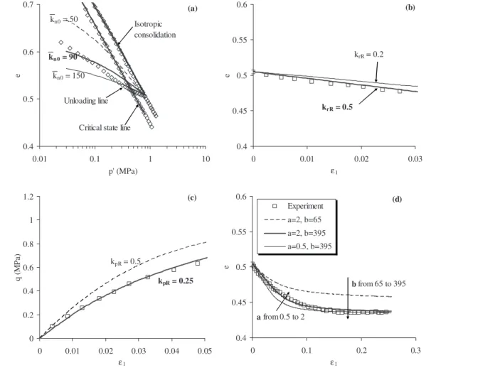
0.4 0.5 0.6 0.7 0.01 0.1 1 10 p' (MPa) e kn0= 50 kn0= 90 kn0= 150 Isotropic consolidation
Critical state line Unloading line (a) 0.4 0.45 0.5 0.55 0.6 0 0.01 0.02 0.03 ε1 e krR= 0.2 krR= 0.5 (b) 0 0.2 0.4 0.6 0.8 1 1.2 0 0.01 0.02 0.03 0.04 0.05 ε1 q (M P a) k pR= 0.5 kpR= 0.25 (c) 0.4 0.45 0.5 0.55 0.6 0 0.1 0.2 0.3 ε1 e Experiment a=2, b=65 a=2, b=395 a=0.5, b=395 (d) a from 0.5 to 2 b from 65 to 395
has also been made for San Francisco Bay Mud to illustrate the ability of this model to predict the behavior of soils with inherent anisotropy.
White Kaolinite Clay
White kaolinite clay is a remolded clay prepared in the laboratory from a mixture of dry clay powder and water. The slurry is then progressively consolidated. The white clay has a plastic limit of about 30% and liquid limit of about 60%. According to scanning electron microscope photos, we assume that the mean cluster size
d is 0.004 mm and the value of N/V is calculated from Eq. 共23兲.
Calibration of Model Parameters
Calibration of the parameters for white kaolinite clay is illustrated in this section. The calibration requires one isotropic compression
test and two drained triaxial compression tests under different confining pressures. The experimental results used for calibration are shown in Fig. 5.
1. Intercluster elastic constants: k¯n0, krRand n—the exponent n
can be determined from stress-strain curves considering very small strains. As reported by Hicher共2001兲, the value is 0.75 for white kaolinite clay. The value of k¯n0can be determined
from Eq. 共24兲, and its calibration is shown in Fig. 6共a兲. krR can be determined from the e-1curve of a drained compres-sion test at a small strain condition, as shown in Fig. 6共b兲, in which the experimental data are taken from Fig. 5共c兲. 2. Intercluster friction angle: and m—the intercluster
fric-tion angle is the slope of the critical state line on the p-q plane, as shown in Fig. 5共b兲. A typical value of 1 is used for m.
3. Intercluster normal hardening rule: cpand kpR—the value of
cpcan be determined from Eq.共26兲 based on the slopes of
Table 1.Model Parameters for Clay
Materials n ecr0 e0 m cp ¯kn0 krR kpR a b
White kaolinite clay 0.75 0.866 0.88 23° 1 0.091 0.022 90 0.5 0.25 2 395
Black kaolinite clay 0.55 1.87 1.84 21° 1 0.238 0.041 45 0.4 0.7 2 350
San Francisco bay mud 0.95 2.283 2.35 31.2° 1 0.1 0.017 300 0.3 0.1 3 225
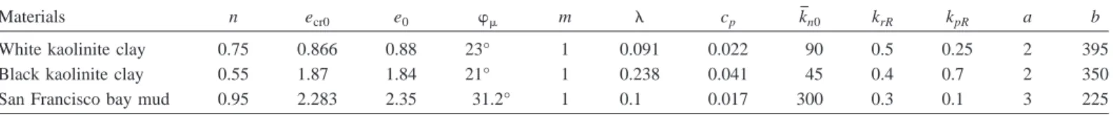
0 0.2 0.4 0.6 0.8 0 0.05 0.1 0.15 ε1 q( M P a) Experiment Simulation (a) OCR = 2 OCR = 1 OCR = 12 Selected 4 steps for
micro-plane's behaviour 0 0.2 0.4 0.6 0.8 0 0.2 0.4 0.6 0.8 1 p' (Mpa) q( M P a) Experiment Simulation (b) OCR = 2 OCR = 1 OCR = 12 1 0.87 Selected 4 steps for
micro-plane's behaviour Step1 Step2 Step3 Step4 -0.2 0 0.2 0.4 0.6 0 0.05 0.1 0.15 ε1 ∆ u( M P a) Experiment Simulation (c) OCR = 2 OCR = 1 OCR = 12 0.4 0.5 0.6 0.7 0.01 0.1 1 p' (MPa) e (d) OCR = 1 Isotropic consolidation Critical state line
OCR = 12
OCR = 2
Fig. 7.Comparison of computed and experimental results for white kaolinite clay in undrained tests:共a兲 stress-strain curves; 共b兲 effective stress paths;共c兲 pore pressure versus axial strain curves; and 共d兲 void ratio versus mean stress curves
the isotropic compression and rebound lines. The value of kpRcan be determined from the q-1curve of a drained com-pression test at a small strain condition as shown in Fig. 6共c兲, in which the experimental data are taken from Fig. 5共a兲. 4. Dilation constants a and b—constants a and b can be
deter-mined from the e-1curve of a drained compression test, as
shown in Fig. 6共d兲. Parameter a controls the magnitude of volume change and parameter b controls the initial slope of the curve.
5. Critical state for the packing: and ecr0.
The value of e0, ecr0and can be determined from the isotro-pic compression line and the critical state line on the e-ln p plane.
0 0.2 0.4 0.6 0.8 0 0.2 0.4 0.6 0.8 1 p' (Mpa) q (MP a) (a) a = 2 a = 5 a = 1 1 M b = 395 0 0.2 0.4 0.6 0.8 0 0.2 0.4 0.6 0.8 1 p' (Mpa) q( M P a) (b) b = 395 b = 65 b = 650 1 M a = 2
Fig. 8.Influence of parameters a and b on undrained stress path
0 0.2 0.4 0.6 0.8 1 0 0.1 0.2 0.3 ε1 q( M P a) Experiment Simulation (a) OCR = 1 OCR = 2 OCR = 4 OCR = 8 Selected 4 steps for micro-plane's behaviour 0 0.2 0.4 0.6 0.8 1 0 0.2 0.4 0.6 0.8 1 1.2 p' (Mpa) q( M P a) Experiment Simulation (b) 1 0.81 OCR = 1 OCR = 2 OCR = 4 OCR = 8
Selected 4 steps for micro-plane's behaviour 0.7 0.8 0.9 1 1.1 1.2 1.3 0 0.1 0.2 0.3 ε1 e Experiment Simulation (c) OCR = 1 OCR = 2 OCR = 4 OCR = 8 0.7 0.8 0.9 1 1.1 1.2 1.3 0.01 0.1 1 10 p' (Mpa) e Experiment Simulation (d) OCR = 1 OCR = 2 OCR = 4 OCR = 8 Isotropic consolidation
Critical state line
Fig. 9.Comparison between predicted and experimental results for black kaolinite clay in drained tests:共a兲 stress-strain curves; 共b兲 stress paths;
The model parameters determined for white kaolinite clay are listed in Table 1.
Drained Tests on Normally Consolidated Clay
Drained triaxial tests on normally consolidated white kaolinite clay have been reported and analyzed by Biarez and Hicher 共1994兲. Two specimens isotropically consolidated up to respec-tively 0.4 and 0.8 MPa, were loaded to failure in drained condi-tion. Using the parameters in Table 1, the predicted test results are plotted in Fig. 5. The stress-strain curves in Fig. 5共a兲 and the void ratio change in Figs. 5共c and d兲 show good agreement between experimental and computed curves. The paths in the e-log p⬘ plane关Fig. 5共d兲兴 show that the void ratio approaches the critical state line when the stress state approaches the failure line in the p-q plane. Since this set of experimental data are used for param-eter calibration, a good comparison is expected.
Undrained Triaxial Tests on Normally and Overconsolidated Clay
Experimental data of undrained triaxial tests on normally and overconsolidated white kaolinite clay specimens were also re-ported by Biarez and Hicher共1994兲. Three samples were isotro-pically consolidated up to 0.8 MPa, and two of them were unloaded to 0.4 and 0.067 MPa, so that the OCRs of the three samples were equal to 1, 2, and 12, respectively. The same mate-rial parameters in Table 1 were used to predict the stress-strain behavior for the three undrained tests.
As shown in Fig. 7共a兲, the computed and measured stress-strain curves are in good agreement. The stress paths shown in Fig. 7共b兲 indicate that for the normally consolidated 共OCR=1兲 and slightly overconsolidated共OCR=2兲 samples, the stress paths do not overpass the critical state line. While, for the strongly overconsolidated specimen共OCR=12兲, the stress path goes above the critical state line, at which dilation occurs, leading to an in-crease of the mean effective stress. The pore pressure develop-ment and e-log p⬘ curves are shown in Figs. 7共c and d兲. The comparisons show good agreement.
It is to be noted that parameters a and b have significant in-fluence on the stress path of undrained test. Fig. 8 shows different effective stress paths as influenced by different values of a and b. Based on the comparison in Fig. 7, the model using parameters calibrated from drained tests is capable of predicting the stress-strain behavior of undrained tests for specimens under different overconsolidation ratios.
Black Kaolinite Clay
Black kaolinite clay is also a remolded clay mixed from clay powder with a darker color. The black kaolinite clay has a plastic limit p= 30%, and liquid limitl= 70%, which is much more
compressible than the white kaolinite clay. The parameters pre-sented in Table 1 are calibrated from triaxial compression tests on normally consolidated specimen, using the method described above. Again, the mean cluster size d is 0.004 mm and the value of N/V is calculated by Eq. 共23兲.
Drained Tests on Overconsolidated Clay
Tests on black kaolinite clay samples were performed by Zervoyanis 共1982兲 and analyzed by Biarez and Hicher 共1994兲.
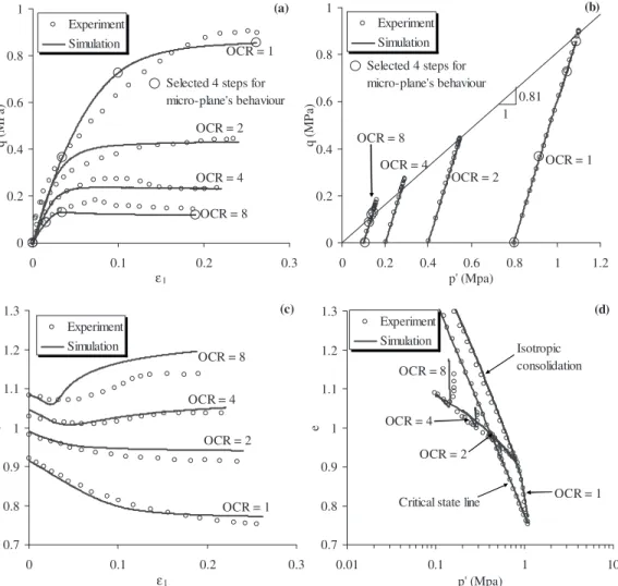
0 0.2 0.4 0.6 0 0.5 1 1.5 σ (Mpa) τ (M Pa ) φ = 21o 18o 28o 45o 72o 55o (a) 0o Selected 4 steps for
micro-planes corresponding to those at global curves
0 0.1 0.2 0.3 0.4 0.5 -0.2 0 0.2 0.4 0.6 γ τ( MP a ) 18o 28o 45o 72o 55o (b) -0.1 0 0.1 0.2 0.3 0.4 0.5 0.6 0 15 30 45 60 75 90 Orientation of micro-planes (o) τ (M Pa ) Predicted values Static hypothesis (c) Step1 Step4 Step3 Step2 0.6 0.8 1 1.2 1.4 1.6 1.8 2 0 15 30 45 60 75 90 Orientation of micro-planes (o) σ (MP a) Predicted values Static hypothesis (d) Step1 Step4 Step3 Step2 -0.1 0 0.1 0.2 0.3 0.4 0.5 0.6 0.7 0 15 30 45 60 75 90 Orientation of micro-planes (o) γ Step1 (e) Step4 Step3 Step2 -0.01 0 0.01 0.02 0.03 0 15 30 45 60 75 90 Orientation of micro-planes (o) ε (f) Step1 Step4 Step3 Step2
Fig. 10.Local stresses and strains on planes of various orientations for drained test on black kaolinite clay共OCR=1兲: 共a兲 local stress paths; 共b兲 local shear stress-strain curves;共c兲 local shear stresses; 共d兲 local normal stresses; 共e兲 local shear strains; and 共f兲 local normal strains
The tests begin with an isotropic consolidation up to 0.8 MPa, then unloaded to 0.4, 0.2, and 0.1 MPa, respectively. The OCRs are 1, 2, 4, and 8, respectively. The predicted void ratio changes in Fig. 9共c兲 show a contractive behavior for OCR=1 and 2, and a dilative behavior for OCR= 4 and 8. The contractive and dilative behaviors can also be seen in the predicted paths on the
e-log p curves in Fig. 9共d兲. For OCR=4 and 8, the stress-strain
curves in Fig. 9共a兲 show strain softening, which corresponds to the stress paths in Fig. 9共b兲 above the critical state line. An over-all good agreement is observed between experimental and pre-dicted results for different OCRs. The two examples of black and white kaolinite clay demonstrate that the model is capable of reproducing with good precision the mechanical behavior of both stiff and soft remolded clays under drained and undrained triaxial test conditions.
Microplane Behavior
The model is capable of describing the intercluster strains for cluster contacts in all orientations. The orientation of a given contact plane is represented by an angle␥ measured from the x axis to the branch vector, as shown in Fig. 4. The angles ␥ se-lected in this study are 18°, 45°, 55°, and 72° respectively共note that the vertical orientation, ␥=0, corresponds to a horizontal contact plane兲. The deformation behavior of the intercluster con-tact planes are discussed here for both drained and undrained conditions.
Drained Conditions
The drained test on black kaolinite clay with OCR= 1 and 3c= 0.8 MPa 共see Fig. 9兲 is selected for showing intercluster
behavior. Four steps are selected for this test关see circles marked on Fig. 9共a兲兴. For each step, the intercluster stress and strain on contacts of various orientations are plotted to show their evolution.
Fig. 10 shows the local stress-strain relationships for the contact planes in the selected orientations. From the - curve 关Fig. 10共a兲兴, we can see that the local stress paths have different slopes for plane orientations from 18° to 72°. The four steps are also marked on each stress path. Under an increase of the vertical stress, the planes oriented near the horizontal direction共i.e., small values of ␥兲 are subjected mainly to a normal stress component ⌬. The shear component becomes more significant when the plane is inclined.
The local shear stress-strain curves 关Fig. 10共b兲兴 show that every plane is mobilized to a different degree. The actively mov-ing planes are located in a narrowly oriented band near the orien-tation of about 55°, which is responsible for the overall deformation of the specimen. Other planes are inactive with small movement. This clearly indicates that the local strains do not uniformly conform to the overall strain of the specimen.
The local stresses plotted in Figs. 10共c and d兲 indicate that the local stresses uniformly conform to the overall stress of the as-sembly, which proves that the static hypothesis 共i.e., j␣=ijni␣兲
used in this model is satisfied in all load steps. The local shear strains plotted in Fig. 10共e兲 indicate that the local shear strains are relatively uniform up to the load Step 2 and become highly nonuniform at Step 3 and Step 4. The largest shear strain occurs on the planes near the orientation at about 55°. Fig. 10共f兲 shows a very small change of the local normal strains during the four load steps. However, at load Step 3 and Step 4, the plot illustrates nonuniform strains, where contraction occurs accompanying the
0 0.02 0.04 0.06 0.08 0.1 0 0.1 0.2 σ (Mpa) τ (M Pa ) φ = 21o 18o 28o 45o 72o 55o (a) 0o Selected 4 steps for micro-planes corresponding to those at global curves
0 0.02 0.04 0.06 0.08 0.1 -0.2 0 0.2 0.4 0.6 0.8 1 γ τ( MP a ) 18o 28o 45o 72o 55o -0.02 0 0.02 0.04 0.06 0.08 0.1 0 15 30 45 60 75 90 Orientation of micro-planes (o) τ (M Pa ) Predicted values Static hypothesis (c) Step1 Step3 Step4 Step2 0 0.1 0.2 0.3 0 15 30 45 60 75 90 Orientation of micro-planes (o) σ (M P a) Predicted values Static hypothesis (d) Step1 Step3 Step4 Step2 -0.2 0 0.2 0.4 0.6 0.8 1 1.2 0 15 30 45 60 75 90 Orientation of micro-planes (o) γ Step1 (e) Step4 Step3 Step2 -0.1 -0.08 -0.06 -0.04 -0.02 0 0.02 0 15 30 45 60 75 90 Orientation of micro-planes (o) ε (f) Step1 Step4 Step3 Step2 (b)
Fig. 11.Local stresses and strains on planes of various orientations for drained test on black kaolinite clay共OCR=8兲: 共a兲 local stress paths; 共b兲 local shear stress-strain curves;共c兲 local shear stresses; 共d兲 local normal stresses; 共e兲 local shear strains; and 共f兲 local normal strains
largest shear strain on the planes near the orientation of 55°. This indicates that a contraction shear band may occur at failure of the normally consolidated clay.
The drained test on black kaolinite clay with OCR= 8 and 3c= 0.1 MPa共see Fig. 9兲 is also selected for showing the inter-cluster behavior. Four load steps are selected for this test 关see circles marked on Fig. 9共a兲兴 to plot intercluster stresses and strains to show their evolution.
The trends of our results are similar to that of OCR= 1. The major difference is that local stresses on some planes can exceed the line of tan due to the interlocking of aggregates in this overconsolidated specimen. Fig. 11共b兲 shows that the plane of the orientation equal to 55° contributes mostly to the deformation of the assembly. The local stress plotted in Figs. 11共c and d兲 indi-cates that the local stresses uniformly conform to the overall stress of the assembly at all steps. The local shear and normal strains plotted in Figs. 11共e and f兲 indicate that the largest shear strain, occurring on the planes near the orientation equal to 55°, is accompanied by large dilation. Thus a dilation shear band may occur at failure for the overconsolidated clay.
Undrained Conditions
The undrained test on white kaolinite clay with OCR= 1 and 3c= 0.8 MPa共see Fig. 7兲 has been selected to demonstrate inter-cluster behavior. Four load steps are also selected for this test关see circles marked on Fig. 7共a兲兴 to show the evolution of local stresses and strains.
From the- curve in Fig. 12共a兲, we can see different local stress paths for undrained loading conditions. The local shear
stress-strain curves 关Fig. 12共b兲兴 show that every plane is mobi-lized to a different degree. The active planes are located in a narrowly oriented band near the orientation of 55°.
The local stresses plotted in Figs. 12共c and d兲 indicate that the local stresses uniformly conform to the overall stress of the assembly, which demonstrates that the static hypothesis 共i.e., j␣=ijni␣兲 is satisfied in all load steps. The local shear strains
plotted in Figs. 12共e and f兲 indicate that the local shear strains are relatively uniform up to the load Step 3, and become highly non-uniform at Step 4. The largest shear strain occurs on the planes near the orientation of 55°, but no specific volume change has been associated with it, because of the constraint of overall zero volume change due to undrained conditions.
Inherent Anisotropy
Natural clay often exhibits anisotropic behavior. Kirkgard共1991兲 performed undrained triaxial test on samples of San Francisco
0 0.1 0.2 0.3 0.4 0 0.2 0.4 0.6 0.8 1 σ (Mpa) τ (M P a) φ = 23o 18o 28o 45o 72o 55o (a) 0o 90o
Selected 4 steps for micro-planes corresponding to those at global curves
0 0.1 0.2 0.3 0.4 -0.2 0 0.2 0.4 0.6 γ τ( MP a ) 18o 28o 45o 72o 55o (b) -0.1 0 0.1 0.2 0.3 0.4 0 15 30 45 60 75 90 Orientation of micro-planes (o) τ (M P a) Predicted values Static hypothesis (c) Step1 Step4 Step3 Step2 0.2 0.4 0.6 0.8 1 1.2 0 15 30 45 60 75 90 Orientation of micro-planes (o) σ (MP a) Predicted values Static hypothesis (d) Step1 Step4 Step3 Step2 -0.1 0 0.1 0.2 0.3 0.4 0.5 0 15 30 45 60 75 90 Orientation of micro-planes (o) γ Step1 (e) Step4 Step3 Step2 -0.006 -0.004 -0.002 0 0.002 0.004 0.006 0 15 30 45 60 75 90 Orientation of micro-planes (o) ε (f) Step1 Step4 Step2 Step3
Fig. 12.Local stresses and strains on planes of various orientations for undrained test on white kaolinite clay共OCR=1兲: 共a兲 local stress paths;
共b兲 local shear stress-strain curves; 共c兲 local shear stresses; 共d兲 local normal stresses; 共e兲 local shear strains; and 共f兲 local normal strains
a0=0 a0=0.6
a0=1
Fig. 13.Distribution of contact orientations with different values of a0
Bay mud to study the degree of anisotropy in this clay deposit. The soil samples were taken from a depth of 6.1 m with a water table depth of 6 m. Gradation analysis showed that the soil con-sists of 55% clay and 45% silt. The soil has the following prop-erties: water content of 98.5%, unit weight of 14.4 kN/m3, specific gravity of 2.55, liquid limit of 1.36, and initial void ratio of 1.35. The samples were tested by applying an axial load in the horizontal and vertical directions to investigate different behav-iors due to material anisotropy.
Material anisotropy is characterized by local material con-stants, which are orientational dependent, and can be expressed as a function of and ␥ 共the two angles in the spherical coordinate system, as shown in Fig. 4兲. To describe such a parameter, a density function E共,␥兲 has been introduced. Integration of E共,␥兲 over all orientations should be equal to 1, i.e.
1 =
冕
0 /2冕
0 2 E共,␥兲sin ␥dd␥ 共28兲 Thus, for an isotropic material, the function E共,␥兲=1/2. For an orthotropic material, the density function can be expanded to a series using the method of spherical harmonic expansion in three dimensions. The truncated form of the series consisting of only second-order terms isE共,␥兲 = 1 2
冉
1 + a0 4共3 cos 2␥ + 1兲 + 3a22sin 2␥ cos 2冊
共29兲 For a cross-anisotropic material, a22becomes equal to zero and Eq.共28兲 is reduced toE共,␥兲 = 1 2
冋
1 +a0
4共3 cos 2␥ + 1兲
册
共30兲 In three dimensions, the inherent anisotropy can be repre-sented by a distribution whose major axis often coincides with vertical or horizontal directions. An example of distributions with different values of a0is shown in Fig. 13. The axes of anisotropy of the soil are identical to those of the axes of loading stresses.It has been found关see Chang and Misra 共1990兲兴 that the an-isotropy can be characterized by a tensor that matches the
coeffi-Horizontal
Sample
Vertical
Sample
1
3
2
Fig. 14.Schematic plot for vertical and horizontal samples
0 0.05 0.1 0.15 0.2 0 0.05 0.1 0.15 0.2 0.25 ε1 q (MP a) Vertical sample Horizontal sample Vertical prediction Horizontal prediction (a) p'i= 0.175 MPa p'i= 0.125 MPa 0 0.05 0.1 0.15 0.2 0 0.05 0.1 0.15 0.2 p' (Mpa) q( M P a) Vertical sample Horizontal sample Vertical prediction Horizontal prediction (b) 0 0.05 0.1 0.15 0.2 0 0.05 0.1 0.15 0.2 0.25 ε1 q( M P a) Vertical sample Horizontal sample Vertical prediction Horizontal prediction (c) p'i= 0.175 MPa p'i= 0.125 MPa 0 0.05 0.1 0.15 0.2 0 0.05 0.1 0.15 0.2 p' (Mpa) q( M P a) Vertical sample Horizontal sample Vertical prediction Horizontal prediction (d)
cients of the spherical harmonic expansion. For example, in the case of a cross anisotropic material, the friction angle can be given by 关兴 = ave
冤
1 + a0 0 0 0 1 −a0 2 0 0 0 1 −a0 2冥
共31兲where ave = average value. In the case of ave= 31.2° and ao= −0.25, the friction angle in the minor axis is1= 23.4° and in the major axes2=3= 35.1°.
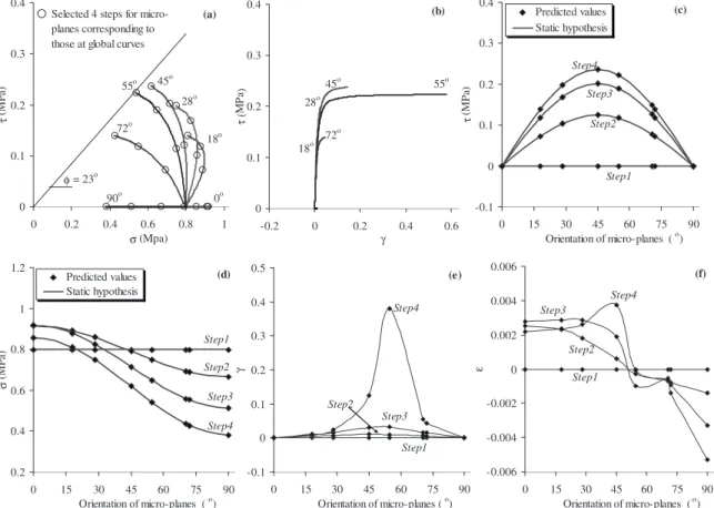
For a soil layer with an inherent anisotropy due to the geologi-cal deposition process, the material properties are usually cross anisotropic, with a symmetry around its major axis that coincides often with the vertical direction. Two samples cored from vertical and horizontal directions are represented schematically as a cube in Fig. 14. The shaded area is perpendicular to the vertical direc-tion 共Direction 1兲. The properties in Directions 2 and 3 are the same, but different from the ones in Direction 1. Using the aver-aged behavior of vertical and horizontal samples, we can calibrate the parameters which are summarized in Table 1.
For the purpose of comparing the predictions with the experi-mental results, two triaxial compression tests were simulated by the model. The two soil samples were isotropically consolidated up to 0.125 and 0.175 MPa, respectively. Afterward, both samples were deviatorically loaded in undrained condition. To model the difference in shear strength for vertical and horizontal samples, we assign the following anisotropy of the friction angle: 3= 35.1° and1= 25.4°. The predicted curves in Fig. 15共a兲 show good agreement with the maximum strength of the two samples. To improve the predicted initial slopes of the undrained stress paths, an additional anisotropy is assigned to the elastic stiffness, 共k¯n0兲1= 600 and共k¯n0兲3= 150. As a result, the predicted undrained stress paths in Fig. 15共d兲 show more difference in the initial slopes between the vertical and horizontal samples, thus showing a better comparison with the experimental results.
Summary and Conclusion
The notion of treating clay clusters as grains makes it promising for extending the well tested methodology of modeling granular material to the modeling of clay. In the newly developed micro-structural model for clay, the overall strain includes plastic sliding and plastic compression among clay clusters. Although the model involves the use of parameters at the scale of clay cluster, we do not need to obtain these parameters directly from experimental tests at this small scale. The parameters can be easily obtained from calibrating two or three conventional triaxial tests on regular size soil specimens.
The model was used to simulate the stress-strain behavior of two different remolded clay. For each type of clay, using the same set of parameters, we could simulate reasonably well both drained and undrained tests. The model was also used to simulate the stress-strain behavior of a natural clay, taking into account its anisotropic nature caused by the clay deposition during geological formation. Based on the model’s performance on these three dif-ferent clays, the microstructural approach seems to be applicable for capturing the effects of confining stress, OCRs, and inherent anisotropy.
References
Batdorf, S. B., and Budianski, B. 共1949兲. “A mathematical theory of plasticity based on concept of slip,” NACA Tech Note 1871. Bazant, Z. P., and Oh, B. H.共1986兲. “Efficient numerical integration on
the surface of a sphere.” J. Appl. Math. Mech., 66共1兲, 37–49. Bazant, Z. P., Xiang, Y., Adley, M. D., Prat, P. C., and Akers, S. A.
共1996兲. “Microplane model for concrete. II: Data delocalization and
verification.” J. Eng. Mech., 122共3兲, 255–262.
Biarez, J., and Hicher, P. Y.共1994兲. Elementary mechanics of soil behav-iour, Balkema, Rotterdam, The Netherlands, 208.
Biarez, J., and Hicher, P. Y.共2008兲. “Mechanisms of soil deformation.” Constitutive modeling of soils and rocks, P. Y. Hicher and J. F. Shao, eds., Wiley, New York, 31–71.
Chang, C. S. 共1988兲. “Micromechanical modeling of constructive rela-tions for granular material.” Micromechanics of granular materials, M. Satake and J. T. Jenkins, eds., Elsevier, Amsterdam, 271–279. Chang, C. S., Chao, S. C., and Chang, Y.共1995兲. “Estimates of
mechani-cal properties of granulates with anisotropic random packing struc-ture.” Int. J. Solids Struct., 32共14兲, 1989–2008.
Chang, C. S., and Gao, J.共1995兲. “Second-gradient constitutive theory for granular material with random packing structure.” Int. J. Solids Struct., 32共16兲, 2279–2293.
Chang, C. S., and Hicher, P.-Y. 共2005兲. “An elastic-plastic model for granular materials with microstructural consideration.” Int. J. Solids Struct., 42, 4258–4277.
Chang, C. S., Kabir, M., and Chang, Y. 共1992a兲. “Micromechanics modelling for the stress strain behavior of granular soil—II: Evalua-tion.” J. Geotech. Engrg., 118共12兲, 1975–1994.
Chang, C. S., and Liao, C.共1990兲. “Constitutive relations for particulate medium with the effect of particle rotation.” Int. J. Solids Struct., 26, 437–453.
Chang, C. S., and Misra, A. 共1990兲. “Application of uniform strain theory to heterogeneous granular solids.” J. Eng. Mech., 116共10兲, 2310–2328.
Chang, C. S., Misra, A., and Acheampon, K.共1992b兲. “Elastoplastic de-formation of granulates with frictional contacts.” J. Eng. Mech.,
118共8兲, 1692–1708.
Chang, C. S., Misra, A., and Weeraratne, S. P.共1989a兲. “A slip mecha-nism based constitutive model for granular soils.” J. Eng. Mech.,
115共4兲, 790–807.
Chang, C. S., Sundaram, S. S., and Misra, A.共1989b兲. “Initial moduli of particulate mass with frictional contacts.” Int. J. Numer. Analyt. Meth. Geomech., 13共6兲, 626–641.
Christofferson, J., Mehrabadi, M. M., and Nemat-Nassar, S. 共1981兲. “A micromechanical description on granular material behavior.” ASME J. Appl. Mech., 48, 339–344.
Delley, B.共1996兲. “High order integration schemes on the unit sphere.” J. Comput. Chem., 17共9兲, 1152–1155.
Emeriault, F., and Cambou, B. 共1996兲. “Micromechanical modeling of anisotropic nonlinear elasticity of granular medium.” Int. J. Solids Struct., 33共18兲, 2591–2607.
Hicher, P. Y.共2001兲. “Microstructure influence on soil behaviour at small strains.” Pre-failure deformation characteristics of geomaterials, M. Jamiolkowski, R. Lancellotta, and D. Lo Presti, eds., Swets and Zeitlinger, Lisse, The Netherlands, 2, 1291–1297.
Hicher, P. Y., Wahyudi, H.and Tessier, D.共2000兲. “Microstructural analy-sis of inherent and induced anisotropy in clay.” Mech. Cohesive-Frict. Mater., 5共5兲, 341–371.
Jenkins, J. T.共1988兲. “Volume change in small strain axisymmetric de-formations of a granular material.” Micromechanics of granular ma-terials, M. Satake and J. T. Jenkins, eds., Elsevier, Amsterdam, 143– 152.
Jenkins, J. T., and Strack, O. D. L.共1993兲. “Mean-field inelastic behavior of random arrays of identical spheres.” Mech. Mater., 16, 25–33. Kirkgard, M. M., and Lade, P. V.共1991兲. “Anisotropy of normally
con-solidated San Francisco bay mud.” Geotech. Test. J., 14共3兲, 231–246. Kruyt, N. P., and Rothenburg, L.共2002兲. “Micromechanical bounds for
the effective elastic moduli of granular materials.” Int. J. Solids Struct., 39共2兲, 311–324.
Lebedev, V. I.共1976兲. “Quadratures on the sphere.” Zh. Vychisl. Mat. Mat. Fiz., 16, 294–306.
Lebedev, V. I. 共1977兲. “Quadrature formulas of orders 25–59 for the sphere.” Sib. Math. J., 18, 132–142.
Liao, C. L., Chan, T. C., Suiker, A. S. J., and Chang, C. S. 共2000兲. “Pressure-dependent elastic moduli of granular assemblies.” Int. J. Numer. Analyt. Meth. Geomech., 24, 265–279.
Liao, C. L., Chang, T. P., Young, D., and Chang, C. S.共1997兲. “Stress-strain relationship for granular materials bases on hypothesis of best fit.” Int. J. Solids Struct., 34共31–32兲, 4087–4100.
Matsuoka, H., and Takeda, K. 共1980兲. “A stress-strain relationship for granular materials derived from microscopic shear mechanisms.” Soils Found., 20共3兲, 45–58.
Mindlin, R. D.共1969兲. “Microstructure in linear elasticity.” Arch. Ration. Mech. Anal., 16, 51–78.
Oda, M.共1977兲. “Coordination number and its relation to shear strength of granular material.” Soils Found., 17共2兲, 29–42.
Ortiz, M., Pinsky, P. M., and Taylor, R. L.共1983兲. “Operator split meth-ods for the numerical solution of the elastoplastic dynamic problem.” Comput. Methods Appl. Mech. Eng., 39, 137–157.
Pande, G. N., and Sharma, K. G. 共1982兲. “Multi-laminate model of clays-a numerical evaluation of the influence of rotation of the
prin-cipal stress axis.” Proc., Symp. on Implementation of Computer Pro-cedures and Stress-Strain Laws in Geotechnical Engineering, C. S. Desai and S. K. Saxena, eds., Acorn, Durham, N.C., 575–590. Rothenburg, L., and Selvadurai, A. P. S.共1981兲. “Micromechanical
defi-nitions of the Cauchy stress tensor for particular media.” Mechanics of structured media, A. P. S. Selvadurai, ed., Elsevier, Amsterdam, 469–486.
Rowe, P. W.共1962兲. “The stress-dilatancy relations for static equilibrium of an assembly of particles in contact.” Proc. R. Soc. London, Ser. A,
269, 500–527.
Simo, J. C., and Hughes, T. J. R. 共1998兲. Computational inelasticity, Springer, New York.
Suiker, A. S. J., and Chang, C. S.共2004兲. “Modelling failure and defor-mation of an assembly of spheres with frictional contacts.” J. Eng. Mech., 130共3兲, 283–293.
Taylor, D. W.共1948兲. Fundamentals of soil mechanics, Wiley, NewYork. Walton, K.共1987兲. “The effective elastic moduli of a random packing of
spheres.” J. Mech. Phys. Solids, 35, 213–226.
Zervoyanis, C.共1982兲. “Etude synthétique des propriétés mécaniques des argiles et des sables sur chemin oedométrique et triaxial de revolu-tion.” Thèse de Docteur-Ingénieur, Ecole Centrale de Paris 共in French兲.