Pre- and post-scheduling memory allocation strategies on MPSoCs

HAL Id: hal-00868945

https://hal.archives-ouvertes.fr/hal-00868945

Submitted on 2 Oct 2013

HAL is a multi-disciplinary open access

archive for the deposit and dissemination of

sci-entific research documents, whether they are

pub-lished or not. The documents may come from

teaching and research institutions in France or

abroad, or from public or private research centers.

L’archive ouverte pluridisciplinaire HAL, est

destinée au dépôt et à la diffusion de documents

scientifiques de niveau recherche, publiés ou non,

émanant des établissements d’enseignement et de

recherche français ou étrangers, des laboratoires

publics ou privés.

Pre- and post-scheduling memory allocation strategies

on MPSoCs

Karol Desnos, Maxime Pelcat, Jean François Nezan, Slaheddine Aridhi

To cite this version:

Karol Desnos, Maxime Pelcat, Jean François Nezan, Slaheddine Aridhi. Pre- and post-scheduling

memory allocation strategies on MPSoCs. Electronic System Level Synthesis Conference (ESLSyn13),

May 2013, Austin, TX, United States. pp.60-65. �hal-00868945�

Pre- and Post-Scheduling Memory Allocation

Strategies on MPSoCs

Karol Desnos, Maxime Pelcat, Jean-Franc¸ois Nezan

IETR, INSA Rennes, CNRS UMR 6164, UEB 20, Av. des Buttes de Co¨esmes, 35708 Rennes email: kdesnos, mpelcat, jnezan@insa-rennes.fr

Slaheddine Aridhi

Texas Instruments France 06271 Villeneuve Loubet, France

email: saridhi@ti.com

Abstract—This paper introduces and assesses a new method

to allocate memory for applications implemented on a shared memory Multiprocessor System-on-Chip (MPSoC).

This method first consists of deriving, from a Synchronous Dataflow (SDF) algorithm description, a Memory Exclusion Graph (MEG) that models all the memory objects of the applica-tion and their allocaapplica-tion constraints. Based on the MEG, memory allocation can be performed at three different stages of the implementation process: prior to the scheduling process, after an untimed multicore schedule is decided, or after a timed multicore schedule is decided. Each of these three alternatives offers a distinct trade-off between the amount of allocated memory and the flexibility of the application multicore execution. Tested use cases are based on descriptions of real applications and a set of random SDF graphs generated with the SDF For Free (SDF3) tool.

Experimental results compare several allocation heuristics at the three implementation stages. They show that allocating memory after an untimed schedule of the application has been decided offers a reduced memory footprint as well as a flexible multicore execution.

I. INTRODUCTION

During the design of an embedded system, memory issues strongly impact the system quality and performance, as the area occupied by the memory can be as large as 80% of the chip and may be responsible for a major part of its power consumption [1]. Consequently, memory allocation plays a crucial role in the implementation process of an application on a Multiprocessor System-on-Chip (MPSoC) and new allo-cation techniques are needed to accommodate the increasing complexity of embedded systems where multiple applications are executed concurrently on a single MPSoC.

This paper focuses on memory allocation of applications described by a Synchronous Dataflow (SDF) Model of Com-putation (MoC) [2]. A SDF MoC models the application as a directed graph of computational entities named actors that exchange data via First In, First Out data queues (FIFOs). Each actor is associated with fixed firing rules specifying its behavior in terms of data token production and consumption. A token is an abstract representation of a data quantum, independent of its size. Actors themselves are “black boxes” of the model and may be implemented in any programming language. Firing an actor consists of starting its preemption-free execution. An example of an SDF graph with 5 actors is given in Figure 1. Edges are labeled with their token production and consumption rates. An edge with a black dot

signifies that initial tokens are present in the FIFO queue when the system starts to execute. The number of initial tokens is specified by the xN label. Initial tokens are a semantic element of the SDF MoC that makes communication possible between successive iterations of the graph execution; they are often used to pipeline applications described with SDF graphs [2].

A

20

B

10

C

50 200 100 150 150

D

40 50 50

E

30 25 50 75 75 x75

Fig. 1. Synchronous Dataflow (SDF) graph

Multicore scheduling is composed of actor mapping, scheduling and timing [3]. Mapping a graph consists of as-signing the computation of each actor to a specific processing element of the architecture. Scheduling consists of ordering the firings of the actors assigned to each processing element. In a timed schedule, not only the order of actor firings is fixed but also the time at which each actor starts and ends its execution. Multicore scheduling stages can be performed at compile time or at runtime.

Section II of this paper presents existing memory allocation techniques. Section III explains the preprocessing of the SDF graph to reveal its memory characteristics. Then, Section IV details the different implementation stages and Section V presents a performance evaluation of our method. Finally, Section VI concludes this paper and proposes directions for future work.

II. RELATEDWORK

Memory optimization for multicore systems has generally been studied as a post-scheduling process. As such, the life-times of the different memory objects of an application are de-rived from scheduling and timing information. Minimization is then achieved by allocating memory objects whose lifetimes do not overlap in the same memory space. Common approaches to perform the memory allocation are:

• Running an online allocation algorithm. Online allocators

assign memory objects one by one in the order in which they arrive. The most commonly used online allocators are the First-Fit (FF) and the Best-Fit (BF) algorithms [4]. FF algorithm consists of allocating an object to the first available space in memory that is sufficiently large to

store it. The BF algorithm works similarly but allocates each object to the available space in memory whose size is the closest to the size of the allocated object.

• Running an offline allocation algorithm [1], [5]. In

con-trast to online allocators, offline allocators have a global knowledge of all memory objects requiring allocation, thus making further optimizations possible.

• Coloring an exclusion graph that models the conflicting

memory objects [6].

• Using constraint programming [7] where memory

con-straints are used together with cost, resource usage and execution time constraints.

The novelty of our memory allocation method is that it is applicable at three different stages of the implementation process. Indeed, memory allocation can be performed before scheduling, after the multicore scheduling process but without actor timing information, or with a timed multicore schedule of the graph actors. As shown in Section IV, these three possibilities offer a trade-off between size of memory footprint and flexibility of actor mapping and scheduling.

III. PREPROCESSING TOWARDMEMORYALLOCATION

Before allocating an SDF graph in memory, a set of transformations is applied to reveal and model its embedded parallelism and its memory characteristics.

A. Transforming the Algorithm

The first transformation applied to the input SDF graph to reveal parallelism is a conversion into a single-rate SDF (srSDF) graph: a SDF graph where the production and con-sumption rates on each FIFO are equal. Each vertex of the srSDF graph corresponds to a single actor firing from the SDF graph. This conversion is performed by computing the topology matrix [2], by duplicating actors by their number of firings, and by connecting FIFOs properly. For example, in Figure 2, actorsB, C, and D are each split in two instances and new FIFOs are added to ensure the equivalence with the SDF graph of Figure 1. An algorithm to perform this conversion can be found in [8].

The second conversion consists of generating a Directed Acyclic Graph (DAG) by isolating one iteration of the algo-rithm. This conversion is achieved simply by ignoring FIFOs with initial tokens in the srSDF. In our example, this approach means that the feedback FIFO C₂ → C₁ which stores 75 initial tokens is ignored.

A

20

E

30

B

1 10

B

2 10

C

1 50

C

2 50

D

1 40

D

2 40 25 25 100 100 150 150 50 50 x75 75 75

Core1 schedule Core2 schedule

Fig. 2. Single-rate SDF (Directed Acyclic Graph if dotpoint FIFO is ignored) Dotpoint arrows depict new precedence relationships introduced by a schedule of the DAG on an architecture with 2 cores.

In the context of memory analysis and allocation, these transformations are applied to fulfill the following objectives:

• Expose data parallelism: Concurrent analysis of data

paral-lelism and data precedence gives information on the lifetime of memory objects prior to any scheduling process. Indeed, two FIFOs belonging to parallel data-paths may contain data tokens simultaneously and are consequently forbidden from sharing a memory space. Conversely, two single-rate FIFOs linked with a precedence constraint can be allocated in the same memory space since they will never store data tokens simultaneously. In Figure 2 for example, FIFO A → B₁ is a predecessor toC₁ → D₁. Consequently, these two FIFOs may share a common address range in memory.

• Break FIFOs into shared buffers: In the SDF model, channels

carrying data tokens between actors behave like FIFO queues. The memory needed to allocate each FIFO corresponds to the maximum number of tokens stored in the FIFO during an iteration of the graph. As this number of tokens depends on the schedule of the actors, methods exist to derive a schedule that minimizes the memory needed to be allocated to the FIFOs [9]. However, in our method, the memory allocation can be independent from scheduling considerations. It is for this rea-son that FIFOs of undefined size before the scheduling step are replaced with buffers of fixed size during the transformation of the graph into a srSDF. In Figure 2, buffers linking two actors will be written and read only once with a data token of fixed size, which simplifies the memory allocation.

• Derive an acyclic model: Cyclic data-paths in an SDF graph

are an efficient way to model iterative or recursive calls to a subset of actors. In order to use efficient static scheduling algorithms [10], SDF models are often converted into DAGs before being scheduled. Besides revealing data-parallelism, this transformation makes it easier to schedule an application, as each actor is fired only once per execution of the resulting DAG. Similarly, in the absence of a schedule, deriving a DAG permits the use of memory objects (communication buffers) that will be written and read only once per execution of the DAG. Consequently, before a memory object is written and after it is read, its memory space will be reusable to store other objects.

B. Extracting Memory Characteristics from the Algorithm

The DAG resulting from the transformations of an SDF graph contains three types of memory objects

• Communication buffers: The first type of memory object,

which corresponds to the single-rate FIFOs of the DAG, are the buffers used to transfer data between consecutive actors. In our approach, we consider that the memory allocated to these buffers is reserved from the execution start of the producer actor until the completion of the consumer actor. This choice is made to enable custom token consumption throughout actor firing time. As a consequence, the memory used to store an input buffer of an actor should not be reused to store an output buffer of the same actor. In Figure 2, the 100 units of memory used to carry data between actorsA and B₁ can not be reused, even partially, to transfer data fromB₁ toC₁.

• Working memory of actors: The second type of memory

object corresponds to the maximum amount of memory allo-cated by an actor during its execution. This working memory represents the memory needed to store the data used during the computations of the actor but does not include the input

buffer nor the output buffer storage. In our method, we assume that an actor keeps an exclusive access to its working memory during its execution. In Figures 1 and 2, the size of the working memory associated with each actor is given by the number below the actor name. This memory is equivalent to a task stack space in an operating system.

• Feedback/Pipeline FIFOs: The last type of memory object

corresponds to the memory needed to store edges ignored as a result of the transformation of a srSDF into a DAG. These edges carry data between successive executions of the DAG and must behave like FIFO queues.

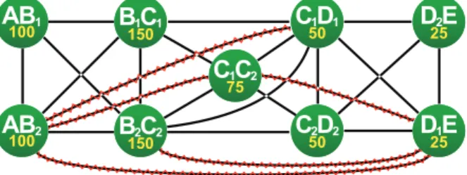
C. Deriving a Memory Exclusion Graph (MEG)

Once an application has been transformed into a DAG and all its memory objects have been identified, the last pre-processing step of our allocation method consists of deriving the MEG [11] used for memory allocation (Section IV).

A Memory Exclusion Graph (MEG) is an undirected weighted graph denoted byG =< V, E, w > where:

• V is the set of vertices. Each vertex represents an

indi-visible memory object.

• E is the set of edges representing the memory exclusions. • w : V → N is a function with w(v) the weight of a

vertex v. The weight of a vertex corresponds to the size of the associated memory object.

• |S| the cardinality of a set S. |V | and |E| are respectively

the number of vertices and edges of a graph.

• δ(G) = _{|V |·(|V |−1)}2·|E| the edge density of the graph corres-ponding to the ratio of existing exclusions to all possible exclusions.

Two memory objects of any type exclude each other (i.e. they can not share the same memory space) if a schedule can be derived from the DAG where both these memory objects store data simultaneously. Some exclusions are directly caused by the properties of the memory objects, such as exclusions between input and output buffers of an actor. Other exclusions result from the parallelism of an application, as is the case with the working memory of actors from parallel data-paths that might be executed concurrently.

The MEG presented in Figure 3 is derived from the SDF graph of Figure 1. The complete MEG contains 18 memory objects and 78 exclusions but, for clarity, only the vertices corresponding to the buffers between actors (1sttype memory objects) are presented. The values printed below the vertices names represent the weightw of the memory objects. Methods to build the MEG are given in [11].

C

1

C

2 75

D

1

E

25

D

2

E

25

C

2

D

2 50

C

1

D

1 50

B

2

C

2 150

B

1

C

1 150

AB

2 100

AB

1 100

Fig. 3. Memory Exclusion Graph (MEG). Crossed out exclusions are removed when considering new precedence edges induced by the schedule of Fig. 2

D. Generating Memory Bounds from MEG

Memory bounds of an SDF graph are introduced in [11] and used in this paper to assess allocation results. The MEG of an application is built and analyzed in order to derive two values that bound the amount of memory needed for the allocation of all memory objects in memory (Figure 4). For example, the memory required for the MEG allocation of Figure 3 is between 525 and 725 memory units.

Insufficient

memory allocated memoryPossible memoryWasted

Available Memory

Lower

Bound≤AllocationOptimal BoundUpper=AllocationWorst 0

Fig. 4. Memory Bounds

This bounding method, independent of timing and archi-tecture constraints, can be used prior to allocation to verify whether a targeted architecture has sufficient memory to run an application. In the next section, we show that a MEG can be updated to incorporate precedence information resulting from a schedule thus allowing the reduction of the amount of allocated memory.

IV. MEMORYALLOCATION

Given an initial MEG constructed from a non-scheduled DAG, we propose three possible implementation stages to perform the allocation of this MEG in shared memory: prior to any type scheduling process, after an untimed multicore scheduling of actors, or after a timed multicore scheduling of the application. The current section details the scheduling flexibility resulting from the three alternatives.

A. Pre-scheduling Memory Allocation

The pre-scheduling memory allocation offers the greatest flexibility of the three alternatives in terms of mapping and scheduling. In this first alternative, the input MEG is allocated in shared memory without being associated with any schedul-ing or timschedul-ing information.

As presented in Section III-C, the MEG models all possi-ble exclusions that may prevent memory objects from being allocated in the same memory space. As we will show in Section IV-B, scheduling a DAG on a multicore architecture always results in removing exclusions from its corresponding MEG but never results in adding new exclusions. Hence, a pre-scheduling MEG models all possible exclusions for all possible multicore schedules of an application. Consequently a compile-time allocation based on a pre-scheduling MEG will never violate any exclusion for any valid multicore schedule of this graph on any shared-memory architecture.

Since a compile-time memory allocation based on a pre-scheduling MEG is compatible with any multicore schedule, it is also compatible with any runtime schedule. The great flexibility of this first allocation approach is that it supports any runtime scheduling policy for the DAG and can accommodate any number of cores that can access a shared memory.

A typical scenario where this pre-scheduling compile-time allocation is useful is a multicore architecture implementation

which runs multiple applications concurrently. In such a sce-nario, the number of cores used for an application may change at runtime to accommodate applications with high priority or those with high processing needs. The compile-time allocation relieves runtime management from the weight of a dynamic allocator while guaranteeing a fixed memory footprint for the application.

The downside of this first approach is that, as shown in the results of Section V, this allocation technique requires substantially more memory than post-scheduling allocators.

B. Post-scheduling Memory Allocation

Post-scheduling memory allocation offers a trade-off be-tween amount of allocated memory and multicore scheduling flexibility. In this second alternative, the input MEG is updated with information from a schedule of the corresponding DAG before allocating the MEG in shared memory.

Scheduling a DAG on a multicore architecture introduces an order of execution of the graph actors, which can be seen as a new precedence relationship between actors. For example, Figure 2 illustrates the new precedence edges that result from scheduling the DAG on 2 cores. In this example,

Core1 executes actorsB2,C1,D2 andE ; and Core2 executes

actors A, B₁,C₂ and D₁. Adding new precedence edges to a DAG results in decreasing the embedded parallelism of the application. For example in Figure 2, the schedule of Core1

creates a new precedence relationship between C₂ andD₁. As presented in Section III-C, memory objects belonging to parallel data-paths may have overlapping lifetimes [11]. Reducing the parallelism of an application results in creating new precedence-paths between memory objects, thus prevent-ing them from havprevent-ing overlappprevent-ing lifetimes and removprevent-ing ex-clusions between them. Since all the parallelism embedded in a DAG is explicit, the scheduling process cannot augment the parallelism of an application and cannot create new exclusions between memory objects. Figure 3 illustrates the updated MEG resulting from the multicore schedule of Figure 2.

The advantage of post-scheduling compared to pre-scheduling allocation is that updating the MEG greatly de-creases its density which results in using less memory to allocate the MEG (Section V).

Like pre-scheduling memory allocation, the flexibility of post-scheduling memory allocation comes from its compat-ibility with any schedule obtained by adding new prece-dence relationships to the scheduled DAG. Indeed, adding new precedence edges will make some exclusions useless but it will never create new exclusions. Consequently, any memory allocation based on the updated MEG of Figure 3 is compatible with a new schedule of the DAG that introduces new precedence edges. For example, we consider a single core schedule derived by combining schedules ofCore₁ andCore₂ as follows A B₂,B₁,C₁,C₂,D₂,D₁ andE . Updating the MEG with this schedule would only result in removing the following exclusions: AB₂−B₁C₁ andC₂B₂−D₁E .

The scheduling flexibility for post-scheduling allocation is inferior to the flexibility offered by pre-scheduling allocation. Indeed, the number of cores allocated to an application may be only dynamically decreased for post-scheduling allocation

while pre-scheduling allocation allows the number of cores to be both dynamically increased and decreased.

C. Timed Memory Allocation

Timed memory allocation offers the least scheduling flex-ibility of the three alternatives. However, this approach is the one that yields the best performance in terms of memory allocation. In this third alternative, the MEG is associated with information from a timed schedule.

A timed schedule is a schedule where not only the ex-ecution order of the actors is fixed, but also their absolute starting and ending times. Such a schedule can be derived if the exact, or the worst-case execution times of all actors are known at compile time [12]. Following assumptions made in Section III-B, the lifetime of a memory object begins with the execution start of its producer, and ends with the execution end of its consumer. In the case of working memory, the lifetime of the memory object is equal to the lifetime of its associated actor. Using a timed schedule, it is thus possible to update a MEG so that exclusions remain only between memory objects whose lifetimes overlap.

A B

Core1

C D

Core2

E F

Core3

(a) Original 3 cores timed schedule

A B

Core1

C

D

Core2

_E

F

(b) 2 cores reschedule with post-scheduling allocation

A

Core1

C

D

Core2

E

B F

(c) 2 cores reschedule with timed allocation

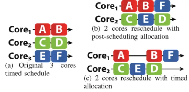
Fig. 5. Re-scheduling from 3 to 2 cores with no precedence between actors

Rescheduling a DAG with a timed memory allocation con-sists of adding precedence edges between all actors with non-overlapping lifetimes. As a consequence, the parallelism of the application is greatly decreased, which leads to less efficient re-scheduling possibilities. Figure 5(a) illustrates this issue with an example where 6 actors, A to F , with no dependency between them are scheduled on 3 cores. Figure 5(b) shows the schedule obtained when rescheduling the 6 actors on 2 cores in the case of post-scheduling memory allocation where actor order from the original schedule must be respected. Figure 5(c) shows the schedule obtained when rescheduling the 6 actors on 2 cores in the case of timed memory allocation where time precedence from the original schedule must be respected. BecauseE must end its execution before B and D are started, this schedule is longer than the schedule obtained with post-scheduling allocation.

Because its MEG has the lightest density, timed allocation has the best results in terms of memory size. However, its reduced parallelism makes it the least flexible scenario in terms of multicore scheduling. The results presented in the next section illustrate the memory allocation efficiency offered by the three implementation stages.

V. RESULTS

The three implementation stages presented in Section IV were tested within the Preesm MPSoC rapid prototyping

framework [12]. For each case, three allocation algorithms were tested to allocate the MEGs in memory: the First-Fit (FF) and the Best-Fit (BF) algorithms [4], and the Placement Algorithm (PA) algorithm introduced by DeGreef et al. in [1]. Two types of memory object orders were used in online algorithms that allocate memory objects in order in which they are received. In the Largest-First (LF) order, memory objects are allocated in decreasing order of size. For post-scheduling and timed allocations, we also tested the allocation of the memory objects in scheduling order. This is equivalent to using an online allocator at runtime.

srSDF graph Memory Exclusion Graph (MEG) Nr Application Actors FIFOs |V | δpre δsch δtim Bmax

1 MPEG4 Enc. 74 143 143 0.80 0.60 0.50 2534479 2 H263 Enc.∗ 207 402 603 0.98 0.76 0.50 5238336 3 MP3 Dec.∗ 33 44 71 0.64 0.55 0.31 363104 4 PRACH 308 897 897 0.94 0.67 0.56 4518961 5 Sample Rate 624 1556 1289 0.50 0.22 0.03 1639 *: Actors of this graph have working memory

TABLE I. PROPERTIES OF THE TEST GRAPHS

The different algorithms and stages were tested on a set of MEGs derived from SDF graphs of real applications. Table I shows the characteristics of the tested graphs. The first three entries of this table, namely MPEG4 Enc., H263 Enc., and

MP3 Dec., model standard multimedia encoding and decoding

applications. The Sample Rate graph models an audio sample rate converter. The MPEG4 Enc., H263 Enc. and Sample Rate graphs were taken from the SDF For Free (SDF3) example database1_{. The PRACH graph models the preamble detection}

part of the Long Term Evolution (LTE) telecommunication standard [12]. Information on the working memory of actors was only available for the MPEG4 Enc. and the MP3 Dec. graphs. In Table I, columns δ_pre,δ_sch, andδ_tim respectively correspond to the density of the MEG in the pre-scheduling, post-scheduling, and timed stages. Bmaxgives the upper bound in Bytes for the memory allocation of the applications [11].

In order to complete these results, the different algorithms were also tested on 45 SDF graphs that were randomly generated with SDF31_{tool. These 45 MEGs cover a wide range}

of complexities with a number of memory objects|V | ranging from 47 to 2208, and exclusion densities δ ranging from 0.03 to 0.98. For each stage, a table presents the performance of the three allocators for each application. Performance is expressed as a percentage corresponding to the amount of memory allocated by the algorithm compared to the smallest amount of memory allocated by all algorithms. So, 0% means that the algorithm determined the best allocation. A positive percentage value indicates the degree of excess memory allocated by an allocator compared to the value of the Best Found column. The B_min column gives the lower memory bound found using the heuristic presented in [11]

For each stage, a box-plot diagram presents performance statistics obtained with all 50 graphs. For each allocator, the following information is given: the leftmost and rightmost marks are the best and worst performance achieved by the allocator, left and right sides of the rectangle respectively are inferior and superior to 75% of the 50 measured performances,

1_{SDF3 website: http://www.es.ele.tue.nl/sdf3}

and the middle mark of the rectangle is the median value of the 50 measured performances.

A. Pre-scheduling allocation

First-Fit (FF) Best-Fit (BF)

Nr Best Found Bmin LF LF PA [1] 1 988470 -3% +3% 0% +13% 2 2979776 0% +1% +1% 0% 3 144384 -3% +2% +2% 0% 4 2097152 0% 0% +1% +29% 5 347 -17% 0% +4% +18% Bmin: Lower bound (Bytes) for the memory allocation of the application [11] LF: Algorithm fed in Largest-First Order

TABLE II. PRE-SCHEDULING MEMORY ALLOCATION

Performances obtained for pre-scheduling allocation are displayed in Table II and Figure 6. These results clearly show that the FF-LF algorithm tends to generate a smaller footprint than the other algorithms. Indeed, the FF-LF algorithm finds the best allocation for 29 of the 50 graphs tested. When it fails to find the best solution, it assigns only 1.35% more memory, on average, than the Best Found allocation. Moreover, the solution of the FF-LF is 4% superior, on average, to the lower bound B_min.

0% 5% 10% 15% 20% 25% 30% 35% 40% 45% 50% 55% FF-LF

BF-LF

PA [1]

Fig. 6. Performance of pre-scheduling allocation algorithms for 50 graphs.

Since the pre-scheduling allocation is performed at compile-time, it is possible to execute all allocation algorithms and keep only the best results. Indeed, in our 50 tests, the BF-LF allocator found the best solution for 13 graphs and the PA for 12 graphs.

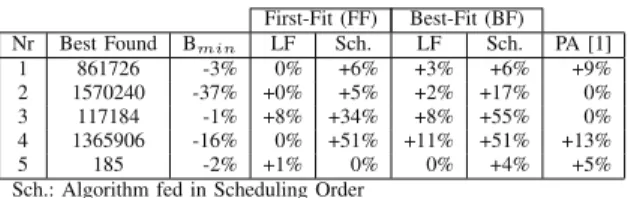
B. Post-scheduling allocation

First-Fit (FF) Best-Fit (BF) Nr Best Found Bmin LF Sch. LF Sch. PA [1]

1 861726 -3% 0% +6% +3% +6% +9% 2 1570240 -37% +0% +5% +2% +17% 0% 3 117184 -1% +8% +34% +8% +55% 0% 4 1365906 -16% 0% +51% +11% +51% +13% 5 185 -2% +1% 0% 0% +4% +5% Sch.: Algorithm fed in Scheduling Order

TABLE III. POST-SCHEDULING MEMORY ALLOCATION

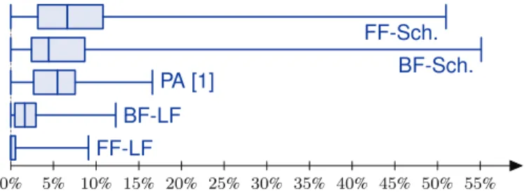
Table III and Figure 7 present the performance obtained for post-scheduling allocation on a multicore architecture with 3 cores. Because the 50 graphs have very different degrees of parallelism, mapping them on the same number of cores decreases their parallelism differently and enables us to have a wide variety of test cases. On average, updating MEGs with scheduling information reduces their exclusion density by 39% which in turns leads to a diminution of the amount of allocated memory by 32%.

As for pre-scheduling allocation, the FF-LF is the most efficient algorithm, finding the best allocation for 29 of the 50

0% 5% 10% 15% 20% 25% 30% 35% 40% 45% 50% 55% FF-LF

BF-LF

PA [1] BF-Sch.

FF-Sch.

Fig. 7. Performance of post-scheduling allocation algorithms for 50 graphs.

graphs and allocating 1.74% more memory, on average, than the Best Found solution for the remaining 21 graphs. Online allocation algorithms fed in scheduling order present the worst performance which was expected since online algorithms do not exploit global knowledge of all memory objects.

C. Timed allocation

Performances obtained for timed allocation are presented in Table IV and Figure 8. The FF-LF allocator is once again the most efficient algorithm as it finds the best allocation for 31 of the 50 graphs, including all 5 real applications.

First-Fit (FF) Best-Fit (BF) Nr Best Found Bmin LF Sch. LF Sch. PA

1 760374 -0% 0% +13% +0% +13% +13% 2 1243072 -0% 0% +28% +10% +48% +3% 3 111008 -3% 0% +3% 0% +3% +1% 4 1231968 -8% 0% +17% +14% +22% +26% 5 41 -10% 0% +5% +5% +2% +17%

TABLE IV. TIMED MEMORY ALLOCATION

The online allocators fed in scheduling order assign more memory than the FF-LF algorithm for 38 graphs with up to 48% more memory being assigned. In the timed stage, online allocators assign only 7% less memory, on average, than the FF-LF algorithm in the post-scheduling stage. In 5 cases, including the PRACH application, online allocators assign even more memory in the timed stage than which was allocated by the FF-LF algorithm in the post-scheduling stage. Considering theO(nlogn) complexity of these online allocators [4], where

n is the number of allocated objects, using the post-scheduling

allocation is an interesting alternative. Indeed, using post-scheduling allocation removes the computation overhead of dynamic online allocation while guaranteeing a fixed memory footprint slightly superior to that which could be achieved dynamically. 0% 5% 10% 15% 20% 25% 30% 35% 40% 45% 50% 55% FF-LF BF-LF BF-Sch. FF-Sch. PA [1]

Fig. 8. Performance of timed allocation algorithms for 50 graphs.

On average, the Best Found timed allocation uses only 11% less memory than the post-scheduling allocations and only

2.7% more memory than the minimum bound B_min. Consid-ering the small gain in footprint and the loss of flexibility induced by this stage (Section IV), timed allocation appears to be a good choice for systems with restricted memory resources where flexibility is not important. However, for systems where the memory footprint is important, but scheduling flexibility is also desired, the post-scheduling allocation offers the best trade-off. Finally for systems where a strong flexibility is essential, the pre-scheduling allocation offers all the required parallelism while ensuring a fixed memory footprint.

VI. CONCLUSION AND FUTURE WORKS

In this paper, we have proposed a new method to perform memory allocation of applications described with SDF graphs. In this method, memory allocation can be performed at three distinct stages of the implementation process, each offering a distinct trade-off between memory footprint and scheduling flexibility. We show that using our method with the First-Fit (FF) allocator fed in the Largest-First (LF) order pro-vides smaller memory footprints that commonly used dynamic online allocators. Furthermore, allocating memory after an untimed schedule of the application has been decided is shown to offer an efficient trade-off between memory footprint and multicore execution flexibility.

Future work on this subject will include a study of the throughput and latency obtained for the different stages of memory allocation. An investigation of a runtime scheduler design that exploits the scheduling flexibility offered by the pre- and post-scheduling allocations is also planned.

REFERENCES

[1] E. de Greef, F. Catthoor, and H. de Man, “Array placement for storage size reduction in embedded multimedia systems,” ASAP, 1997. [2] E. Lee and D. Messerschmitt, “Synchronous data flow,” Proceedings of

the IEEE, vol. 75, no. 9, pp. 1235 – 1245, sept. 1987.

[3] E. A. Lee and S. Ha, “Scheduling strategies for multiprocessor real-time dsp,” in Global Telecommunications Conference, 1989, and

Exhi-bition. Communications Technology for the 1990s and Beyond. GLOBE-COM’89., IEEE. IEEE, 1989, pp. 1279–1283.

[4] D. S. Johnson, “Near-optimal bin packing algorithms,” Ph.D. disserta-tion, Massachusetts Institute of Technology, 1973.

[5] P. Murthy and S. Bhattacharyya, “Shared memory implementations of synchronous dataflow specifications,” in DATE Proceedings, 2000. [6] M. Bouchard, M. Angalovi´c, and A. Hertz, “About equivalent interval

colorings of weighted graphs,” Discrete Appl. Math., vol. 157, pp. 3615– 3624, October 2009.

[7] R. Szymanek and K. Kuchcinski, “A constructive algorithm for memory-aware task assignment and scheduling,” in CODES

Proceed-ings, ser. CODES ’01. New York, NY, USA: ACM, 2001, pp. 147–152.

[8] S. Sriram and S. S. Bhattacharyya, Embedded Multiprocessors:

Schedul-ing and Synchronization, 2nd ed. Boca Raton, FL, USA: CRC Press, Inc., 2009.

[9] W. Sung and S. Ha, “Memory efficient software synthesis with mixed coding style from dataflow graphs,” VLSI Systems, IEEE Transactions

on, no. 5, oct. 2000.

[10] Y.-K. Kwok, “High-performance algorithms of compile-time scheduling of parallel processors,” Ph.D. dissertation, Hong Kong University of Science and Technology, 1997.

[11] K. Desnos, M. Pelcat, J. Nezan, and S. Aridhi, “Memory bounds for the distributed execution of a hierarchical synchronous data-flow graph,” in

SAMOS Proceedings, 2012.

[12] M. Pelcat, S. Aridhi, J. Piat, and J.-F. Nezan, Physical Layer Multi-Core

Prototyping: A Dataflow-Based Approach for LTE eNodeB. Springer Publishing Company, Incorporated, 2012.