HAL Id: hal-02193272
https://hal.archives-ouvertes.fr/hal-02193272
Submitted on 9 Apr 2020
HAL is a multi-disciplinary open access
archive for the deposit and dissemination of
sci-entific research documents, whether they are
pub-lished or not. The documents may come from
teaching and research institutions in France or
abroad, or from public or private research centers.
L’archive ouverte pluridisciplinaire HAL, est
destinée au dépôt et à la diffusion de documents
scientifiques de niveau recherche, publiés ou non,
émanant des établissements d’enseignement et de
recherche français ou étrangers, des laboratoires
publics ou privés.
Multi-task transfer learning for timescale graphical
event models
Mathilde Monvoisin, Philippe Leray
To cite this version:
Mathilde Monvoisin, Philippe Leray. Multi-task transfer learning for timescale graphical event models.
15th European Conference on Symbolic and Quantitative Approaches to Reasoning with Uncertainty
(ECSQARU 2019), 2019, Belgrade, Serbia. �10.1007/978-3-030-29765-7_26�. �hal-02193272�
Graphical Event Models
Mathilde Monvoisin, Philippe Leray
Universit´e de Nantes, LS2N UMR CNRS 6004, Nantes, France [email protected]
Abstract. Graphical Event Models (GEMs) can approximate any smooth multivariate temporal point processes and can be used for capturing the dynamics of events occurring in continuous time for applications with event logs like web logs or gene expression data. In this paper, we propose a multi-task transfer learning algorithm for Timescale GEMs (TGEMs): the aim is to learn the set of k models given k corresponding datasets from k distinct but related tasks. The goal of our algorithm is to find the set of models with the maximal posterior probability. The procedure encourages the learned structures to become similar and simultaneously modifies the structures in order to avoid local minima. Our algorithm is inspired from an universal consistent algorithm for TGEM learning that retrieves both qualitative and quantitative dependencies from event logs. We show on a toy example that our algorithm could help to learn related tasks even with limited data.
Keywords: Graphical Event Model (GEM), Transfer Learning, Multi-task Learning (MTL), Multivariate temporal point process, Process Min-ing
1
Introduction
While probabilistic graphical models such as Dynamic Bayesian Networks [5, 7] allow modeling of temporal dependencies in discrete time, some recent works are dedicated to modeling continuous time processes, with for instance, Contin-uous Time Bayesian Networks [10], Poisson Networks [12], Conjoint Piecewise-Constant Conditional Intensity Models [11].
In [6], Gunawardana and Meek have introduced Graphical Event Models (GEMs) that generalize such models, and Timescale GEM (TGEMs) which are GEMs where the temporal range and granularity of each temporal dependency is made explicit. TGEMs provide a way to understand temporal relationships between some variables, through a graph whose nodes are those variables and whose edges are the dependencies between them. In the case that the observed phenomena is a sequence of events, we can call it a process, so nodes are events and an edge between nodei and nodej means that the appearance of eventi has
In the same work, they have proposed an asymptotically consistent greedy algorithm to learn the structure and parameters of one single TGEM from an event log file. However, one may want to learn multiple processes that might be close. In order to complete this goal, multi-task transfer learning [3] is useful since it allows to learn k related models from k corresponding data sets.
In this paper, we propose an algorithm for transfer learning with TGEM, to allow simultaneous Multi Task Learning (MTL), inspired from Niculescu’s method for MTL [8, 9] with Bayesian Networks. Section 2 is a recall of the back-ground elements useful afterwards, which include Timescale Graphical Event Models definition and current learning methods. Section 3 explains the global strategy used for learning multiple TGEMs, and proposes a method for likeli-hood and prior calculation in order to find the k structures that maximize the posterior probability of the structures given the data. Finally, a toy example in Section 4 illustrates the interest of MTL on TGEMs and Section 5 concludes on the contribution of this paper and the perspectives of research afterwards.
2
Background
This section is a reminder about formal definition of TGEMs and about the greedy search algorithm used for TGEM learning. More details about TGEM definition and learning can be found in Ref. [6].
The data D we use for learning consists in a timed sequence of events until time t∗:
D = {(t1, l1), ..., (ti, li), ..., (tn, ln)}, (1)
where t0 = 0 < ti < ti+1 < t∗ and 1 ≤ i ≤ n − 1. li are labels from a finite
vocabulary. The history h(t) at any time t is the subset of events that occurred before t.
2.1 Timescale Graphical Event Models
A Timescale Graphical Event Model M = (G, T ) is a probabilistic graphical model that can represent data D as given above, using conditional intensity functions. The directed graph G = (L, E) represents the dependencies between events, with L the labels of the events, E the edges of the graph. T = {Te}e∈E
associates each edge e to a list of consecutive timescales Te where |Te| ≥ 1. A
timescale has the form (a, b], with a ≥ 0 and b > a.
We call temporal range the moment during which the timescales of some parent has an impact on the child node. On Fig. 1, the temporal range of A on C takes place between t and t − 2 with a certain intensity and between t − 2 and t − 4 with another one.
In all the models generalizing in the GEM family, the conditional intensity function is used to specify how the present depends on the past in an evolutionary process. This conditional intensity λl of a given event is usually a
A
B C
(0, 2], (2, 4]
Fig. 1. One example of TGEM. L = {A, B, C}, E = {AC} and T = {TAC =
(0, 2], (2, 4]}. The occurrence of event C at time t will depend on possible occurrence of A in time windows [t-4, t-2) and [t-2, t). The occurrences of A and B are independent from other events.
λl(t|h) = λl,Cl(h,t) where the index Cl(h, t) is the parent count vector of l: the
number of occurrences of the parents in the timescales. For the entire paper, we consider that every element of Cl(h, t) is either 0 or 1, thus only the fact that a
parent has occurred or not within the corresponding timescale is important. The marginal likelihood of a TGEM M according to data D can be computed at any time t, as defined in [6]:
p(D|M, λ) =Y l∈L Y j∈pcv λnt,l,j(D) l,j e −λl,jdt,l,j(D), (2)
with nt,l,j(D) and dt,l,j(D) respectively the total, at time t, number of
occur-rences of the event l within its parents configuration j, and duration of this configuration.
2.2 Learning TGEM for a Single Task
Single Task Learning (STL) consists in finding the optimal TGEM (its graph G and its timescales T ) from a dataset D as defined in Section 2.1.
A greedy BIC procedure for TGEM structure learning has been proven as asymptotically consistent in [6]. This strategy is to maximize the BIC score by performing the search on two stages, a Forward search by adding edges and refining the suitability of the timescales, and a Backward search which simplifies the model and deletes unnecessary edges.
The Forward search starts from the empty model M0 and computes the
neighborhood until convergence to finally reach the model MF S. The
neighbor-hood NF S(M) of M is computed with the three operators (add, split and extend )
defined below. M0 ∈ NF S(M) ⇔ ∃O ∈ O = {Oadd(e), Osplit(Te), Oextend(e)}
such as O(M) = M0.
The Backward search starts with MF S and generates all neighbors M0 ∈
NBS(M) such as O(M0) = M until convergence.
The BIC score used for the structure learning procedure is, at time t∗:
BICt∗(M) = log p(D|M, λt∗(D)) −
X
l∈L
|Cl| log t∗, (3)
with λt∗(D) the optimal parameters obtained by likelihood estimation and |Cl|
The subfamily of TGEMs used by the structure learning procedure is called Recursive Timescale Graphical Event Models. A RTGEM refers to any TGEM that can be reached by performing recursively the following operators, starting from an empty model.
The add edge operator Oadd(e) takes as input an edge to be added to the
graph with the default timescale T = (0, hdef] with hdef the default horizon. The
split timescale operator Osplit(Te) takes as input a timescale (a, b] of a specific
existing edge and substitutes it by (a,a+b2 ], (a+b2 , b]. The extend horizon operator Oextend(e) takes as input an existing edge with horizon h and adds a timescale
to this edge (h, 2h] to double its horizon.
Gunawardana and Meek [6] have also proven than RTGEMs can approximate any non-explosive non-deterministic smooth marked point process with finite horizon.
2.3 Distance Between Two RTGEMs
In order to estimate the distance between two RTGEMs, Antakly and al. [1] have proposed an extension of the usual Structural Hamming Distance. The distance between two RTGEMs M1 = ((L, E1), T1) and M2 = ((L, E2), T2) with the
same set of labels, is defined by:
d(M1, M2) = X e∈Esd 1 + X e∈Einter d(T1,e, T2,e), (4)
where Esd are the edges that are present in just one of the two models, and
Einter are present in both models. Ti,eare the timescales for edge e in model Mi
and viis the list of endpoints1of model Mi. The distance between the timescales
is defined by:
d(T1,e, T2,e) =
vnid
vnid+ vid
, (5)
where vnid = |v1\v2| + |v2\v1| and vid = |v1∩ v2| is the number of endpoints
that exist respectively in one and two of timescales T1,e and T2,e.
2.4 Example of Single Task Learning
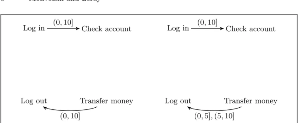
The aim of this example is to illustrate the previously introduced notions. We consider the two models of user behavior on e-banking sites described by the underlying RTGEMs MR1 (Fig. 2) and MR2 (Fig. 3). We also consider that we have (relatively small) web logs D1 and D2 for both sites.
The procedure when considering 2 models separately is to apply the Forward-Backward search introduced in Section 2.2, with a default horizon of edge h = 10. Figure 4 (resp. 5) describes the RTGEM MST L1 (resp. MST L2 ) obtained at the end of this STL algorithm applied to the event log D1 (resp. D2).
1 It is another way of representing timescales. T = (0, a], (a, b], (b, c] is equivalent to
Log out
Log in Check account
Transfer money (0, 10] (0, 5] (0, 10] (0, 10], (10, 20] Fig. 2. Model MR1 Log out
Log in Check account
Transfer money (0, 5] (0, 5], (5, 10] (0, 5] Fig. 3. Model MR2 Log out
Log in Check account
Transfer money (0, 10]
(0, 5]
(0, 10]
Fig. 4. Model MST L1 learned from D1
Log out
Log in Check account
Transfer money (0, 5]
(0, 5], (5, 10]
(0, 5]
Fig. 5. Model MST L2 learned from D2
This single task learning doesn’t take advantage of similarities between both tasks, and can lead to inaccurate results when there is a lack of data. For instance, in this toy example, the event log D1is not sufficient to identify the dependence
between Check Account and Transfer Money in MST L1 .
3
Learning Multiple RTGEMs for Related Tasks
3.1 Problem Statement
In the previous section, we were interested in learning one single RTGEM from one single dataset. We now want to learn a set Sbest = {M∗1, . . . , M∗k} of k
RTGEMs from k datasets D = {D1, . . . , Dk}. The datasets contains event logs
as defined in Section 2.1, with overlapping labels L =Tk
q=1Lq 6= ∅.
We are then interested in maximizing the posterior probability of the set of models given the data:
According to Bayes rules, this posterior probability is proportional to the prior of the models and the marginal likelihood of the set:
p(M1, . . . , Mk|D1, ..., Dk) ∝ p(M1, ..., Mk)p(D1, ..., Dk|M1, ..., Mk). (7)
When considering a priori parameters independence, the marginal likelihood over the set of models can be factorized into the product of the marginal likeli-hood of each data set, and our problem statement can now be expressed as:
Sbest= argmaxM1,...,Mk(p(M1, ..., Mk)
k
Y
q=1
p(Dq|Mq)). (8)
In order to solve this task, we have to compute the marginal likelihood of each model Mq, as well as the prior of the joint distribution over the models M1...Mk
and finally we need a strategy to find the best set.
3.2 Marginal Likelihood
It was demonstrated by Chickering and Heckerman in [4] that the marginal log-likelihood of a Bayesian Network can be approximated by its BIC score. We will conjecture in this paper that the same approximation can be made for Timescale Graphical Event Models, which is the approximation made by [6] and [2]. For a model Mq at time t∗, the marginal log-likelihood log p(Dq|Mq) can
be approximated by the BIC score defined in equation (3) (Section 2.2).
3.3 Prior
The probability p(M1, . . . , Mk) is called the prior because it represents the a
priori knowledge of how similar the models might be. The two extreme cases are therefore, if the models have to be:
– independent: p(M1, . . . , Mk) =Q k
q=1p(Mq),
– equal: p(M1, . . . , Mk) should be 1 if there is no difference between models,
and 0 otherwise.
The solution offered in [8] for Bayesian Networks is to use a constant δ ∈ [0, 1] that penalizes every difference between the models structure when calculating the prior. Niculescu-Mizil and Caruana propose two different priors: one of them considers the minimum number of modifications necessary to make each edge the same in every structure (Edit Prior), and the other one considers the differences per pair of structures (Paired Prior). However, finding the minimum of edits to make all the edges the same is more difficult in TGEMs than in Bayesian Networks. Indeed, there are only two possibilities (present, not present) when considering an arc of a Bayesian Network, while the search space for a single arc of a TGEM is infinite because of the timescales that can always be split
or extended. For this reason, the prior we suggest for TGEM learning is an adaptation of the Paired Prior and is defined as follows:
p(M1, ..., Mk) = Zδ,k Y 1≤q≤k p(Mq) 1 1+(k−1)δ Y 1≤q<q0≤k (1 − δ)d(Mq ,Mq0 )k−1 , (9)
where Zδ,k is a normalization constant and d(Mq, Mq0) is the distance between
two RTGEMs introduced in Section 2.3. In transfer learning context, all the models may not have identical labels. However, for the distance computing, we will only consider shared labels from both models Linter = L1∩ L2 where
M1= ((L1, E1), T1) and M2= ((L2, E2), T2).
The choice of the penalty δ affects the prior such as the higher δ, the closer the models have to be. When δ = 0, the differences d(Mq, Mq0) will not affect
p(M1, . . . , Mk), so the models are considered as independent. When δ = 1, any
distance other than zero between the models makes p(M1, . . . , Mk) = 0 so the
models have to be equal if we want a non-zero prior.
3.4 Finding the Best Set
The strategy named MTL Forward-Backward search that we propose to learn multiple TGEMs is inspired from the one proposed for Single Task Learning in Section 2.2. The strategy uses two steps, one MTL Forward search (algorithm 1) that starts from an empty set S0 (i.e. a set of empty graphs) and one MTL
Backward search (algorithm 2) that starts with the set SF S resulting from the
MTL Forward search.
The scoring function p(S|D) optimized here is obtained from equation (8) with the posterior distribution defined in equation 9 and a marginal log-likelihood approximated by the BIC score defined in equation (3).
Algorithm 1 MTL Forward search Input: D = {D1, · · · Dk}, S0
Output: SF S
1: S ← S0
2: repeat
3: ref ined ← false 4: for S0∈ NF S(S) do
5: if p(S0|D) > p(S|D) then 6: S ← S0
7: ref ined ← true 8: end if
9: end for 10: until not ref ined 11: SF S← S
12: return SF S
Algorithm 2 MTL Backward search Input: D = {D1, · · · Dk}, SF S Output: SBS 1: S ← SBS 2: repeat 3: coarsened ← false 4: for S0∈ NBS(S) do 5: if p(S0|D) > p(S|D) then 6: S ← S0
7: ref ined ← true 8: break
9: end if 10: end for
11: until not coarsened 12: SBS← S
Log out
Log in Check account
Transfer money (0, 10]
(0, 10]
Log out
Log in Check account
Transfer money (0, 10]
(0, 5], (5, 10]
Fig. 6. S = {M1, M2}, set of models obtained during MTL Forward search
As highlighted in [9], changing only one model in the set at each iteration will usually weakly increase the score function or will lead to local optima, so our greedy algorithm has to test modifications in several models at the same time. For this reason, the neighborhoods NF S(S) or NBS(S) are generated thanks to
the three operators (add, split and extend ) introduced in Section 2.2, but applied to all the possible subsets of models in S.
As also observed by Niculescu-Mizil and Caruana for Bayesian Networks, the size of a set of models neighborhood grows much faster than the size of a single model neighborhood. However, the search of the best solution in each neighborhood can be optimized by using a Branch and Bound algorithm, in a similar way to [9], that we can not describe here due to a lack of space.
4
Toy Example of Multi Task Learning
Let us take the simple example (labels are identical) used in Section 2.4, and consider now a Multi Task Learning by applying the MTL Forward-Backward search proposed in Section 3. It is not necessary that the labels are the same, just that they overlap. Figure 6 describes the set of RTGEMs {M1, M2}) jointly
obtained at the end of the third iteration of the MTL Forward phase. The optimal sequence of operators was:
1. M1,2:Oadd(Log in, Check account) (adding the edge in both models),
2. M1,2:Oadd(Transfer money, Log out) (adding the edge in both models),
3. M2:Osplit(Transfer money, Log out, (0,10]) (splitting the edge in M2only).
Let us develop now the next step of this phase. As usual in greedy algo-rithms, the neighborhood of S, NF S(S), will be explored in order to find the
next considered set of models. This neighborhood consists in all the pairs of models {M1, M2} generated from S by applying one single operator to M1
only, M2only, and both M1 and M2.
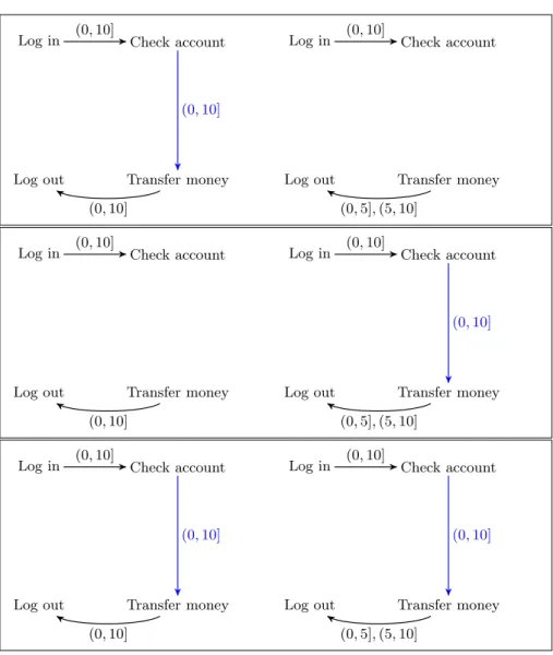
Each box in Fig. 7 contains one neighbor of S corresponding to the operator Oadd(Check account, Transfer money) applied to M1 only, M2 only, or both
Log out
Log in Check account
Transfer money (0, 10]
(0, 10]
(0, 10]
Log out
Log in Check account
Transfer money (0, 10]
(0, 5], (5, 10]
Log out
Log in Check account
Transfer money (0, 10]
(0, 10]
Log out
Log in Check account
Transfer money (0, 10]
(0, 10]
(0, 5], (5, 10]
Log out
Log in Check account
Transfer money (0, 10]
(0, 10]
(0, 10]
Log out
Log in Check account
Transfer money (0, 10]
(0, 10]
(0, 5], (5, 10]
Fig. 7. Some neighbors of S during MTL Forward search: considering to add an edge between Check account and Transfer money (Oadd(Check account, Transfer money))
to M1 only, M2 only, or both M1 and M2 and respectively leading to (from top to
bottom) S1, S2 and S12.
We consider now our objective function (equation (8)) with the Paired prior of equation (9) for our set of two models to determine which of the neighbors will be the one selected for the next step of the phase.
In a need for simplicity, we assume that p(M1) = p(M2). To select the most
likely set, we look for
argmaxM1,M2(p(D1|M1) · p(D2|M2) · (1 − δ)
The distance between the models M1and M2on the sets S, S1, S2and S12.
from figures 6 and 7 are dS1(M1, M2) = dS2(M1, M2) =
4
3 and dS(M1, M2) =
dS12(M1, M2) =
1 3.
pS1(D1|M1) < pS(D1|M1), and M2is the same in both S1and S. From
pre-vious calculations of distances, we know that the penalty term (1 − δ)dS(M1,M2)
is higher than (1 − δ)dS1(M1,M2), so S
1has a lower posterior than S.
We assume that there is a strong dependency between Check account and Transfer money in D2, that makes the presence of the arc from Check account
to Transfer Money in M2 more likely than its absence in M1. We can express
it with: pS12(D1|M1) pS2(D1|M1) >pS12(D2|M2) pS2(D2|M2) . (11) Therefore, from (1 − δ)13 > (1 − δ) 4
3 and equation (11), S12 happens to be
more likely than S2, and both are better sets than S. Finally, S12 is selected for
the next step of the MTL Forward search and the edge between Check Account and Transfer Money is now present in M1 when it was not considered in MST L1
because of the lack of data.
We can see in this example that using our Multi-task learning algorithm can help to learn several related tasks even with limited data by using information from their related tasks.
5
Conclusion
Multi Task Learning is one kind of Transfer Learning, well studied in Machine Learning, but no so developed for probabilistic graphical models such as Bayesian Networks. Graphical Event Models are probabilistic graphical models dedicated to modeling continuous time processes. Single Task Learning such models from event logs have been very recently studied in a few works.
In this paper we proposed an algorithm for Multi Task Learning with Time-scale Graphical Event Models. This algorithm, MTL Forward-Backward search, is an adaptation of the one proposed for Bayesian networks by [9] that also combines the efficient TGEM structure learning method proposed by [6] and the TGEM distance recently proposed in [1]. In this preliminary work, we also illustrated this algorithm with a simple toy example in order to give the intuition of its interest.
In the future, we plan to finalize the implementation of our algorithm, and to apply it on real world case studies in computer security. We also look forward to generalize this approach to another very recent GEM approach (Proximal GEM)[2].
We are also interested in studying beyond Multi-task learning and looking at other Transfer Learning tasks for Graphical Event Models, and dealing with both Incremental and Transfer Learning.
References
1. Antakly, D., Delahaye, B., Leray, P.: Graphical event model learning and verifica-tion for security assessment. In: 32th Internaverifica-tional Conference on Industrial En-gineering and Other Applications of Applied Intelligent Systems, IEA/AIE 2019, Graz, Austria, July 9-11. pp. ?–? Springer International Publishing (2019) 2. Bhattacharjya, D., Subramanian, D., Gao, T.: Proximal graphical event models. In:
Bengio, S., Wallach, H., Larochelle, H., Grauman, K., Cesa-Bianchi, N., Garnett, R. (eds.) Advances in Neural Information Processing Systems 31. pp. 8136–8145. Curran Associates, Inc. (2018)
3. Caruana, R.: Multitask learning: A knowledge-based source of inductive bias. In: Proceedings of the Tenth International Conference on Machine Learning. pp. 41– 48. Morgan Kaufmann (1993)
4. Chickering, D., Heckerman, D.: Efficient Approximation for the Marginal Like-lihood of Incomplete Data given a Bayesian Network. In: UAI’96. pp. 158–168. Morgan Kaufmann (1996)
5. Dean, T., Kanazawa, K.: A model for reasoning about persistence and causation. Computational Intelligence 5(2), 142–150 (1998)
6. Gunawardana, A., Meek, C.: Universal models of multivariate temporal point pro-cesses. In: Gretton, A., Robert, C.C. (eds.) Proceedings of the 19th International Conference on Artificial Intelligence and Statistics. Proceedings of Machine Learn-ing Research, vol. 51, pp. 556–563. PMLR, Cadiz, Spain (09–11 May 2016) 7. Murphy, K.: Dynamic Bayesian Networks: Representation, Inference and Learning.
Ph.D. thesis, University of california, Berkeley (2002)
8. Niculescu-Mizil, A., Caruana, R.: Inductive transfer for bayesian network structure learning. In: Meila, M., Shen, X. (eds.) Proceedings of the Eleventh International Conference on Artificial Intelligence and Statistics. Proceedings of Machine Learn-ing Research, vol. 2, pp. 339–346. PMLR, San Juan, Puerto Rico (21–24 Mar 2007) 9. Niculescu-Mizil, A., Caruana, R.: Inductive transfer for bayesian network structure learning. In: Guyon, I., Dror, G., Lemaire, V., Taylor, G., Silver, D. (eds.) Proceed-ings of ICML Workshop on Unsupervised and Transfer Learning. ProceedProceed-ings of Machine Learning Research, vol. 27, pp. 167–180. PMLR, Bellevue, Washington, USA (02 Jul 2012)
10. Nodelman, U., Shelton, C., Koller, D.: Continuous time Bayesian networks. In: Proceedings of the Eighteenth Conference on Uncertainty in Artificial Intelligence (UAI). pp. 378–387 (2002)
11. Parikh, A.P., , Meek, C.: Conjoint modeling of temporal dependencies in event streams. In: UAI Bayesian Modelling Applications Workshop (August 2012) 12. Rajaram, S., Graepel, T., Herbrich, R.: Poisson-networks: A model for structured
point processes. In: Proceedings of the Tenth International Workshop on Artificial Intelligence and Statistics (January 2005)