HAL Id: inria-00346528
https://hal.inria.fr/inria-00346528
Submitted on 11 Dec 2008
HAL is a multi-disciplinary open access
archive for the deposit and dissemination of
sci-entific research documents, whether they are
pub-lished or not. The documents may come from
teaching and research institutions in France or
abroad, or from public or private research centers.
L’archive ouverte pluridisciplinaire HAL, est
destinée au dépôt et à la diffusion de documents
scientifiques de niveau recherche, publiés ou non,
émanant des établissements d’enseignement et de
recherche français ou étrangers, des laboratoires
publics ou privés.
Mounir Bechchi, Guillaume Raschia, Noureddine Mouaddib
To cite this version:
Mounir Bechchi, Guillaume Raschia, Noureddine Mouaddib. Joining Distributed Database
Sum-maries. [Research Report] RR-6768, INRIA. 2008, pp.29. �inria-00346528�
a p p o r t
d e r e c h e r c h e
0249-6399 ISRN INRIA/RR--6768--FR+ENG Thème SYMJoining Distributed Database Summaries
Mounir Bechchi — Guillaume Raschia — Noureddine Mouaddib
N° 6768
2008
Centre de recherche INRIA Rennes – Bretagne Atlantique
Mounir Bechchi
∗, Guillaume Raschia
∗, Noureddine Mouaddib
†Thème SYM — Systèmes symboliques Équipe-Projet Atlas
Rapport de recherche n° 6768 — 2008 — 26 pages
Abstract: The database summarization system coined SEQ provides
multi-level summaries of tabular data stored into a centralized database. Sum-maries are computed online with a conceptual hierarchical clustering algorithm. However, in many companies, data are distributed among several sites, either homogeneously (i.e. , sites contain data for a common set of features) or het-erogeneously (i.e. , sites contain data for different features). Consequently, the current centralized version of SEQ is either not feasible or even not desirable due to privacy or resource issues.
In this paper, we propose two new algorithms for summarizing hetero-geneously distributed data without a prior "unification" of the data sources:
Subspace-Oriented Join Algorithm (SOJA) and Tree Alignement-based Join Algo-rithm (TAJA). The main idea of such algoAlgo-rithms consists in applying innovative joins on two local models, computed over two disjoint sets of features, to
pro-vide a global summary over the full feature set without scanning the raw data.
SOJA takes one of the two input trees as the base model and the other one is
processed to complete the first one, whereas TAJA rearranges summaries by levels in a top-down manner.
Then, we propose a consistent quality measure to quantify how good our joined hierarchies are. Finally, an experimental study, using synthetic data sets, shows that our joining processes (SOJA and TAJA) result in high quality clustering schemas of the entire distributed data and are very efficient in terms of computational time w.r.t. the centralized approach.
Key-words: Database Summary, Distributed Clustering
∗Atlas-Grim,INRIA/LINA-Université de Nantes †Université Internationale de Rabat
Données
Résumé : Le système SaintEtiQ permet de construire, à partir d’une table
rela-tionnelle, une hiérarchie de concepts résumant cette relation. Les résumés sont générés via un algorithme de classification incrémental et chacun d’entre eux fournit une représentation concise par le biais d’un ensemble de descripteurs linguistiques sur chaque attribut d’une partie des n-uplets de la relation ré-sumée. Les multiples niveaux de granularité qu’offre la structure hiérarchique permettent, a posteriori, d’exhiber une forme résumée de la relation à un niveau de précision voulu.
Actuellement, dans les grandes organisations, les données sont géographiqu-ement distribuées sur plusieurs sites de manière homogène (i.e. , fragmentation horizontale) ou hétérogènes (i.e. , fragmentation verticale). La répartition des données rend inapplicable la procédure de classification conceptuelle telle que définie par SaintEtiQ puisqu’elle exige que les données soient disponibles sur le serveur des résumés; cette hypothèse étant techniquement non satisfiable (i.e. , bande passante, espace de stockage, performance, etc. ) ou trop intrusive (i.e. , confidentialité).
Ce travail propose deux algorithmes pour résumer deux relations hétérogèn-es sans accéder aux donnéhétérogèn-es d’origine: SOJA (Subspace-Oriented Join Algorith-m) et TAJA (Tree Alignement-based Join AlgorithAlgorith-m). Ces deux algorithmes prennent en entrée deux résumés générés localement et de manière autonome sur deux sites distincts et les combinent pour en produire un résumant la re-lation correspondante à la jointure des deux rere-lations locales. Les résultats ex-périmentaux montrent que SOJA et TAJA sont plus performants que l’approche centralisée (i.e. , SaintEtiQ appliqué aux relations après regroupement et join-ture sur un même site) et produisent des hiérarchies semblables à celles que produit l’approche centralisée.
1 Introduction
Because of the ever increasing amount of information stored each day into databases, users can no longer have an exploratory approach for visualizing, querying and analyzing their data without facing the problem often referred to as "Information Overload". Means to circumvent those problems include data reduction techniques and, among them, the SEQ [19] database summarization model which is considered in this paper.
SEQ enables classification and clustering of structured data stored into a database. It applies a conceptual clustering algorithm for partitioning the incoming data in an incremental and dynamic way. The algorithm takes a relational table as input and produces a hierarchical data structure that shows how clusters are related. By cutting the hierarchy at a desired level, a partition-ing of data items into disjoint groups are obtained. Thus, the main concern in the clustering process is to reveal the organization of patterns into "sensible" groups, which allow us to discover similarities and differences, as well as to derive useful conclusions about them. This idea is applicable in many fields [8], such as life sciences, medical sciences and engineering.
Actually, data are often distributed across institutional, geographical and or-ganizational boundaries rather than being stored in a centralized location. Data can be distributed by separating objects or attributes: in the homogeneous case, sites contain subsets of objects with all attributes, while in the heterogeneous case sites contain subsets of attributes for all objects. Because of concerns related to confidentiality, storage, communication bandwidth and/or power limitation, the current centralized version of SEQ is not appropriate for such an environment. For instance, in medical database, only anonymous and statistical information is available since individual information (such as name, address and phone number) can violate patient confidentiality. Even if privacy is not an obstacle, transmitting the entire local data set to a central site and performing the clustering is, in some application areas, quite difficult if not almost impossible. In astronomy, for instance, data sets gathered by telescopes and satellites, spread all over the world, are measured in gigabytes and even terabytes.
The requirement to extract useful information from these databases, with-out pooling the whole data, has led to the new research area of Distributed Knowledge Discovery [16]. In this paper, we propose two new algorithms for summarizing heterogeneously1 distributed data: Subspace-Oriented Join
Algo-rithm (SOJA) and Tree Alignement-based Join AlgoAlgo-rithm (TAJA). Given two
hier-archical clustering schemas (local models) computed over two disjoint sets of features, the main idea of such algorithms consists in applying innovative joins on local models in order to provide a single summary hierarchy over the full feature set without scanning the raw data.
The main concern of this work is to introduce and compare those approaches and list the pros and cons of each one. This raises some questions:
1. How can we define the set of the best representatives (or summaries) of a given data set according to the partial summaries?
2. What are the main critera (time complexity, model consistency, etc.) that need to be taken care of in order to ensure that the join process overcomes the SEQ limitations in distributed systems?
3. How good are the joined hierarchies?
The rest of the paper is organized as follows. In the next section we present the SEQ model and discuss how our proposal can be extended to any grid-based hierarchical clustering algorithm. Then, in Section 3 we define the problem of summarizing distributed heterogeneous data and present some straightforward approaches to address such problem. Two alternative ap-proaches that overcome straightforward apap-proaches limitations are presented in Section 4. Section 5 introduces how to evaluate the correctness of joining algorithm results using an appropriate and consistent clustering validity index. Moreover, an experimental study is detailed in Section 6. Section 7 presents the related work. Finally, in Section 8, we give concluding remarks and future directions of our work.
2 Overview of the SEQ System
Our work relies on the summaries provided by the SEQ system described in [19]. In this section, we introduce the main ideas of the summary model and give useful definitions and properties regarding our proposal. Then, we discuss how our proposal can be extended to any grid-based hierarchical clustering algorithm.
2.1 A Two-Step Process
SEQ (SEQ) is an incremental process that takes tabular data as input and produces multi-resolution summaries of records. Each record, which goes through a mapping step followed by a summarization step, contributes in progressively building the final hierarchy of summaries.
2.1.1 Mapping Service (MSEQ)
SEQ system relies on Zadeh’s fuzzy set theory [25], and more specifically on linguistic variables [14] and fuzzy partitions [15], to represent data in a concise form. The fuzzy set theory is used to translate records in accordance with a Knowledge Base (KB) provided by the user. Basically, the operation replaces the original values of each record in the table by a set of linguistic descriptors defined in the KB. For instance, with a linguistic variable on the attribute INCOME (Figure 1), a value t.INCOME = 440.86e is mapped to
{0.3/tiny, 0.7/very small} where 0.3 is a membership grade that tells how well
the label tiny describes the value 440.86. Extending this mapping to all the attributes of a relation could be seen as mapping the records to a grid-based multidimensional space. The grid is provided by the KB and corresponds to the user’s perception of the domain.
Thus, tuples of table 1 are mapped into two distinct grid-cells denoted by
c1 and c2 in table 2. young is a fuzzy label a priori provided by the KB on
Figure 1: Fuzzy linguistic partition defined on the attribute INCOME
of raw values. The "tuple count" column gives the proportion of records in R that belong to the cell and 0.3/tiny says that tiny fits the data only with a small degree (0.3). It is computed as the maximum of all membership grades of tuple values to tiny in c1.
Table 1: Raw data (R) ID AGE INCOME
t1 22 440, 86
t2 19 542, 12
t3 24 661, 29
Table 2: Grid-cells mapping
Cell AGE INCOME Extent tuple count
c1 young 0.3/tiny t1, t2 0.4
c2 young very small t1, t2, t3 2.6
Flexibility in the vocabulary definition of KB permits to express any single value with more than one fuzzy descriptor and avoid threshold effect thanks to a smooth transition between two descriptors. The mapping of all tuples leads to the point where some tuples become indistinguishable when read using the descriptors. They are then grouped into the multidimensional grid-cells such that there are finally many more records than cells. Each new (coarser) tuple stores a record count and attribute-dependant measures (min, max, mean, standard deviation, etc.). It is then called a summary.
It is worth noticing that a grid of relatively small cells will lead to a greater precision in the summary description. However, the larger the size of a cell, the smaller the precision, hence the difficulty to approximate the exact values of the database records that are represented by any particular cell.
2.1.2 Summarization Service (CSEQ)
Summarization service is the last and the most sophisticated step of the S-EQ system. It takes grid-cells as input and outputs a collection of summaries hierarchically arranged from the most generalized one (the root) to the most specialized ones (the leaves). Summaries are clusters of grid-cells, defining hyperrectangles in the multidimensional space. In the basic process, leaves are grid-cells themselves and the clustering task is performed on L cells rather than
From the mapping step, cells are introduced continuously in the hierarchy with a top-down approach inspired of D.H. Fisher’s Cobweb, a conceptual clustering algorithm [22]. Then, they are incorporated into best fitting nodes descending the tree. Three more operators could be apply, depending on partition’s score U, that are create, merge and split nodes. They allow developing the tree and updating its current state. U is a combination of two well-known measures: typicality [18] and contrast [23]. Those measures maximize between-summary dissimilarity and within-between-summary similarity. Figure 2 represents the summary hierarchy built from the cells c1and c2.
Figure 2: Example of SEQ hierarchy
2.2 Features of the Summaries
Definition 1 Summary Let R be a relation defined over a set E ={A1, . . . , AN} of
attributes. Each attribute Ai ∈ E is defined on a domain DAi. Assume that the
N-dimensional space A1× A2× . . . × ANis equipped with a gridG[E] that defines basic
N-dimensional areas, called cells, in E. The cells are obtained by partitioning every initial feature domain into several sub-domains using linguistic labels from the KB. A summary z (denoted by z⊆ E) of a relation R is the bounding box of a cluster of cells populated by records of R.
The above definition is constructive since it proposes to build generalized summaries (hyperrectangles) from cells that are specialized ones. In fact, it is equivalent to performing an addition on cells such that:
z = c1+ c2+. . . + cm
where ci∈ G[E] is the set of the m cells (summaries) covered by z.
A summary z is then an intentional description associated with a set of tuples
Rzas its extent and a set of cells Lz ∈ P(G[E]), that are populated by records of Rz. P(G[E]) is the set of subsets of G[E]. Hereafter, we shall use LRz and Lz
interchangeably to denote the set of cells populated by records of Rz.
Thus, summaries are areas of E with hyperrectangle shapes provided by
KB. They are nodes of the summary tree built by the SEQ system.
Definition 2 Summary Tree A summary tree HR over R is a collectionZ of
sum-maries verifying:
• ∀z, z&∈ Z, z ! z&⇐⇒ Rz⊆ Rz&;
The relation overZ (i.e. !) provides a generalization-specialization rela-tionship between summaries. And assuming summaries are hyperrectangles in a multidimensional space, the partial ordering defines nested summaries from the larger one to single cells themselves.
In order to provide the end-user with a reduced set of representatives from the data, we need to extract a subset of the summaries in the tree. The straight-forward way of performing such a task is to define a summary partitioning.
Definition 3 Summary Partitioning The set P of leaves of every rooted sub-tree of
the summary hierarchy HRprovides a partitioning of relation R.
We denote by Pzthe top-level partition of z in the summary tree. It is then the most general partitioning of Rzwe can provide from the tree. Note that the most specialized one is the set of cells covering Rz, that is Lz. A partitioning can be obtained a posteriori to set the compression rate depending on user needs. For instance, general trends in the data could be identified in the very first levels of the tree, whereas precise information has to be looked for around leaf-level. Moreover, such partitioning verifies two basic properties: disjunction and coverage.
Property 1 Disjunction
Summaries z and z&are disjoint iff∃i ∈ [1..N], z.Ai∩ z&.Ai=∅.
According to this property, summaries of a partition do not overlap with each other, if we except the overlapping of fuzzy cells borders.
Property 2 Coverage
R =∪z∈PRz
A partition P guarantees complete coverage of relation R since, by definition, representatives of every branch are included into P.
2.3 Time complexity of SEQ
In this section, we discuss the efficiency of the SEQ process and specif-ically, its summarization serviceCSEQ. The mapping serviceMSEQ will not be further discussed as it is a straightforward rewriting process.
The time cost TCSEQofCSEQprocess can be expressed as:
TCSEQ(L) = kSEQ· L · logdL
where L is the number of cells of the output hierarchy, d its average width and logdL an estimation of its average depth. In the above formula, coefficient kSEQ corresponds to the set of operations performed to find the best learning operator to apply at each level of the hierarchy.
Note that the number of leaves L is bounded by pN (i.e. , the size of the grid-based multidimensional space) where p represents the average number of descriptors defined for each feature in E. Of course, the exact number will greatly depend on the data set, and more specifically, on the existing correlations between attribute values. For example, in a car database with attributes product and price, it is likely that we will not find the combination of Ferrari and Cheap.
2.4 The General Case
In the remainder of this paper, we adopt the SEQ system (SEQ) to illustrate our joining algorithms of local models. However, our proposal can be generalized to any clustering technique (e.g. , STING [24], CLIQUE [1]) that is based upon two main functions: a mapping functionM and a hierarchical clustering functionC.
Definition 4 Mapping (M)
Let E ={A1, . . . , AN} be a set of features and assume that the N-dimensional space
A1× A2× . . .× ANis equipped with a gridG[E] that defines basic N-dimensional areas
called cells in E. The cells are obtained by partitioning each initial feature domain into several sub-domains. A mappingM is defined as follows:
M : I(R[E]) → P(G[E])
R .→ M(R) = LR
where I(R[E]) is the set of instances of the relational schema R(A1, . . . , AN) and, for
R∈ I(R[E]), LRis the set of cells populated by records of R.
Definition 5 Hierarchical clustering function (C)
A hierarchical clustering functionC takes a set of cells X as input and outputs a set of subsets of X.C is defined as follows:
C : P(G[E]) → P2(G[E])
X .→ C(X)
whereC(X) verifies the following conditions: (1) X ∈ C(X); (2) ∅ ! C(X); (3) ∀x ∈ X, {x} ∈C (X); (4) ∀c, c&∈ C(X), c ∩ c&∈ {c, c&,∅}. Finally, for every inner node c of the
the hierarchy, c is defined w.r.t. the objective function ofC and the control strategy
used to search in the features space.
Assume X is the result of a mapping process over a relation R (i.e. , X = M(R)), then the elements of C ◦ M(R) are nodes of the grid-based hierarchical clustering schema built byC over R.
As one can observe, SEQ is an instance ofC ◦M . Indeed, M is the mapping serviceMSEQdefined in Section 2.1.1, whereasC is the summarization serviceCSEQof Section 2.1.2 (i.e. , SEQ =CSEQ◦ MSEQ).
Note that SEQ provides a near-optimal partitioning schema for a given data set R since the tree is updated locally every time a new cell is incorporated. However, the best partitioning schema HRof R can be obtained by substituting the summarization serviceCSEQby the following greedy algorithm COPT:
1. search for optimal partitioning Pbestof LR; Pbestis then the top-level parti-tion in the tree HRand is connected to the root z;
2. for each z&∈ Pbestdo
• nothing if z&is a leaf, else
We define here the optimality of Pbest as the result of performing the fol-lowing process (the search strategy) on a set of summariesZ: (1) compute the partition latticeL of Z; (2) for each partition P ∈ L, build summary descriptions (hyperrectangles) from clusters of cells; (3) filter fromL the set of candidate summary partitions P that satisfy the disjunction property (coverage is trivial); (4) the optimal partitioning ofZ is the partition Pbest ∈ P with the highest U value. U is a heuristic objective function, the partition utility (or quality), based on contrast and typicality of summary descriptions [19].
COPTprovides optimal hierarchy by construction but it is exponential w.r.t. the number L of cells in the output hierarchy since it relies on finding the best partition Pbestof various data sets with nesting constraints. This principle requires to explore all the possible partitions each time. The time complexity ofCOPTverifies TCOPT(L) = kOPT· BL, where kOPTis a constant factor andB is the
Lth Bell number2. Thus, T
COPTis O(2L) and consequentlyCOPT is inappropriate
for scaling.
CSEQandCOPTdiffer in the control strategy used to explore the features space, but the objective function U is the same.
In the following section, we formally define the problem of summarizing distributed heterogeneous data and we introduce a running example that will be used throughout this document. Then, we describe the very first ideas to address such a problem and we present their limitations.
3 Problem Analysis
3.1 Problem Statement
To keep things simple, in what follows, we assume that there exist two relational database tables R1 and R2 located respectively on distant sites S1 and S2. R1
and R2are defined respectively on disjoint feature sets E1 ={A1, . . . , AN1} and
E2 = {AN1+1, . . . , AN1+N2}. Furthermore, we assume that there is a common
feature ID, accessible to S1 and S2, that can be used to associate a given
sub-tuple in site S1 to a corresponding sub-tuple in site S2. Note that the latter
assumption is required for a reasonable solution to the distributed clustering problem and is not overly restrictive. Indeed, any entity resolution method could give such association [3, 20].
Definition 6 Problem Definition We define the problem of heterogeneous distributed
data clustering for a clustering algorithmC ◦ MSEQ as follows. Let R1 " R2 be the
natural3 join of R
1 and R2. The problem is to find the global hierarchical clustering
schema HR1"R2of data located at S1and S2over the full feature set E = E1∪ E2, such
that:
(i) HR1"R2=COPT◦ MSEQ(R1" R2) (consistency requirement)
(ii) The entire data transfer is avoided (limited data access requirement)
2B
L="Li=0−1(CLi−1· Bi) gives the number of partitions of a setZ with L elements according to the usual definition.
3The join of R
In addition to requirements (i) and (ii), the proposed solution must also scale well with respect to the number of records and the number of dimensions in large data sets (efficiency requirement).
The traditional solution to the above problem is to transfer R1 and R2 to
one centralized site where the join R1 " R2is performed, and then the global
hierarchy is computed by applyingCOPT◦MSEQover R1" R2. Such an approach
does not satisfy the (ii) and efficiency requirements. Indeed, it uses raw data and it causes high response times since TCOPT∈ O(2L) where L is the number of
cells populated by records of R1 " R2. We therefore discuss new algorithms
which take two local models (i.e. , HR1and HR2) as input instead of the raw data
(i.e. , R1 and R2) and output a single summary tree HR1"R2 based on the two
local models.
3.2 Running Example
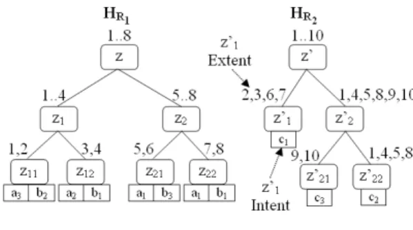
To illustrate our proposal, we introduce two relations R1(A, B) and R2(C) defined
respectively on feature sets E1={A, B} and E2={C}. We consider that {a1, a2, a3},
{b1, b2, b3} and {c1, c2, c3} are sets of linguistic labels defined respectively on the
attributes A, B and C. Furthermore, we assume the existence of unique indices ID to link R1and R2records. Applying SEQ on each of the two relations
leads to the summary trees shown on Figure 3.
Figure 3: HR1and HR2
MSEQ(R1) andMSEQ(R2) as well as their relationship are shown on Table 3.
Table 3: Relationship between R1and R2
IDs MSEQ(R1) 1,2 < a3, b2> 3,4 < a2, b1> 5,6 < a1, b3> 7,8 < a1, b1> IDs MSEQ(R2) 2,3,6,7 < c1> 9,10 < c3> 1,4,5,8 < c2>
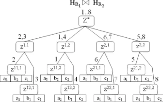
Figure 4 shows the summary hierarchy HR1"R2provided by SEQ when
Figure 4: SEQ on R1" R2
3.3 Basic Approaches
In this section, we discuss the first ideas for joining two summary hierarchies and describe their drawbacks. But before proceeding further, we define new operators that will be used in the following.
Join Operators
Definition 7 Summary Join Operator (") Let z# 1and z2be respectively summaries
of E1and E2(i.e. , z1⊆ E1and z2⊆ E2). We define a join operator for z1and z2as:
z!= z1"z# 2⇐⇒ Rz! = Rz1" Rz2
z!is area of E = E
1∪ E2. Its extent contains records of the restricted natural
join between Rz1 and Rz2. It is worth noticing that the summary join could be
empty (i.e. , z! =∅) as soon as R
z1 and Rz2 have no common values on the ID
attribute (i.e. , Rz1" Rz2=∅).
Definition 8 Partition Join Operator ($") Let P1be a partitioning of R1and P2a
partitioning of R2. The join of P1and P2is defined as:
P1$"P2=
%
z1"z# 2| z1#"z2#∅ ∧ (z1∈ P1)∧ (z2∈ P2)
&
P1$"P2is a partitioning of R1 " R2. Indeed, we can easily check that P1$"P2
verifies the disjunction and coverage properties. We denote by P1$$P2the set
of summaries of P1 such that for each z1 ∈ P1$$P2 there exists z2 ∈ P2 such
z1#"z2∈ P1$"P2.
The intentional content of each joint summary z! = z
1"z# 2 can be obtained
without any mapping process (Section 2.1.1). Indeed, if z1and z2are both cells,
their intents can be appended to form z!intent (e.g. see figure 5). Otherwise,
the intentional description of z!is computed from both sets of cells covered by
z1and z2as follows:
z!= '
c∈(Lz1$"Lz2)
Figure 5: z! = z 11#"z&1
Note that the exact values of attribute-dependent (e.g. , mean, maximum, minimum and standard deviation) and attribute-independent (e.g. , record count) statistical information of each joint cell c#"c&cannot be computed
with-out either centralization of data or communication between sites since such pa-rameters are calculated directly from data. However, if univariate-distribution laws (e.g. , normal, uniform, etc.) of attributes values in c and c& are known (e.g. , STING [24]), an approximation of c#"c&attribute-dependent measures can
be calculated. An approximation of c#"c&attribute-independent parameters is
a bit more complicated, but not impossible. First, the multivariate-distribution law is approximated using the univariate-distribution laws. Then, it could be used to estimate c#"c&attribute-independent measures.
As a consequence to the above definitions, the mapping function MSEQ verifies the following property:
Property 3
MSEQ(R1" R2) = LR1$"LR2=MSEQ(R1)$"MSEQ(R2) .
According to this property, the set of cells of HR1"R2 can be obtained from
both sets of cells of local models HR1and HR2. It means no mapping process is
needed.
Greedy Joining Algorithm (GJA)
The straightforward way of building a global hierarchical clustering schema of
R1" R2without scanning the raw data is to useMSEQproperty (property 3) to computeCOPT◦ MSEQ(R1 " R2) and consequently avoid the explicit mapping
process:
COPT◦ MSEQ(R1 " R2) =COPT(MSEQ(R1)$"MSEQ(R2))
For instance, Figure 6 illustrates the joined hierarchy obtained from sum-mary trees shown in Figure 3 according to the Greedy Joining Algorithm.
GJA provides the optimal hierarchy and does not require scanning of raw
data. However, it does not satisfy the efficiency requirement. Indeed, when assuming|LR1| 3| LR2| 3 l, TGJAis defined as:
TGJA(l) = kGJA· l2+ TCOPT(l2)
where kGJA is a constant factor and TCOPT(l2) is the time cost required to
pro-cess LR1$"LR2 usingCOPT (see Section 2.4). In the above formula, l2 gives the
maximum number of cells populated by records of R1 " R2.
Hence, TGJAis O(2L), where L is the number of cells populated by records of
Figure 6: GJA on HR1and HR2
It is worth noticing that there is no efficient method for computing the opti-mal hierarchy. A search strategy cannot be both computationally inexpensive and construct clusters of high quality. Thus, in the following, our problem’s consistency requirement is relaxed by requiring only an approximation of the optimal joined hierarchy. The counterpart is that we must provide evidences of the quality of the approximate solution (see Section 5.2).
SEQ -based Join Algorithm (SEQ-JA)
One direction to overcome the GJA limitation is to processMSEQ(R1)$"MSEQ(R2)
usingCSEQ(Section 2.1.2) instead ofCOPT.
The joined hierarchy of summary trees from Figure 3 according to SEQ-JA is the same than the one provided by SEQ when performed on R1" R2
(Figure 4). Note that this is not always the case since different sorts of the cells may yield different clustering schemas.
The time complexity of SEQ-JA, when considering|LR1| 3 |LR2| 3 l, is given
by:
TSEQ−JA(l) = kSEQ−JA· l2+ TCSEQ(l2)
where kSEQ−JA is a constant factor and TCSEQ(l2) is the time cost required to
process LR1$"LR2usingCSEQ(see Section 2.3).
Hence, TSEQ−JAis O(L· log L), where L is the number of cells populated by
records of R1 " R2.
Note that SEQ-JA considers all the dimensions of the centralized data set in attempt to build the global schema. Indeed, it does not exploit existing hierarchical partitioning schemas that are pre-computed locally; it takes a set of cells as input and builds the global schema from scratch. Thus, SEQ-JA is expected to break down rapidly as the number of dimensions increases since
TSEQ−JAis quasi-linear w.r.t. the number of cells (i.e. , the size of the grid-based
multidimensional space), which depends on the number of features.
The following alternatives try to achieve high quality clustering schemas of the entire distributed data set as well as to enhance join process performance, exploiting the full capacity of all distributed resources.
4 Alternative approaches
In this section, we present three alternative algorithms in order to overcome the limitations of basic approaches. The Subspace-Oriented Join Algorithm (SOJA) and the SOJA with Rearrangements (SOJA-RA) modify one of the two input trees, called the base model, according to the other one to build a single tree. The last approach, so-called Tree Alignement-based Join Algorithm (TAJA), relies on a recursive processing that performs a join of summary partitions guided by levels of the input hierarchies.
4.1 Subspace-Oriented Join Algorithm
Howto
The main idea of this approach is rather simple. It starts from an existing hier-archical clustering schema within a subspace of the whole data set. Then, once items become indistinguishable from one-another according to this subspace, it proceeds with a sequence of refinements on the existing clusters according to the complementary subspace. More precisely, SOJA assumes one of the two in-put trees as the base model (e.g. , HR1) and the other one (e.g. , HR2) is processed
to refine cells (or leaves) of the first one.
Thus, SOJA1→2(i.e. , HR1is the base model) computes the hierarchy HR1"R2
from HR1and HR2as follows:
1. for each cell c1of HR1, compute LR2$${c1} and do
a. if LR2 $${c1} = ∅ (i.e. , Rc1 " R2 =∅): remove c1from HR1 since it is
populated by records that are not in R1" R2and then, if the parent
of c1has one single child, replace it by the child itself, else
b. if LR2$${c1} = {c2} (i.e. , is a singleton): replace c1with c1"c# 2, else
c. process the set of cells LR2$${c1} using CSEQand replace each node
z of the hierarchyCSEQ(LR2$${c1}) by c1" z then, replace c# 1with the
result tree;
2. build intent, extent and statistical information on the overall features set for each node z of the result hierarchy (the tree obtained once all cells of
HR1have been processed) based on leaves (cells) of the sub-tree rooted by
z (i.e. , z ="c∈Lzc).
The computation of LR2$${c1} is based on a depth-first search and relies on
a strong property of the hierarchy: the generalization step in the SEQ model guarantees that a tuple is absent from a summary’s extent if and only if it is absent from any partition of this summary. This property of the hierarchy permits branch cutting as soon as it is known that no result will be found. Regarding the cell (of the base tree) processed, only a part of the hierarchy is explored.
For instance, Figure 7 illustrates the joined hierarchy obtained from sum-mary trees shown in Figure 3 according to SOJA1→2.
Figure 7: SOJA1→2on HR1and HR2
Discussion
Assume that|LR1| 3 |LR2| 3 l. The time complexity TSOJAof this approach is
defined as follows:
TSOJA(l) = l· [kSOJA·dl− 1
− 1+ TCSEQ(l)] + k&SOJA·
l2− 1
d− 1
where kSOJAand k&SOJAare constant factors and d is the average width of HR1
and HR2. In the above formula, [kSOJA·dl−1−1 + TCSEQ(l)] is the time cost required
to process each cell of the base tree (search for cells from the second tree that would join with current cell and cluster them usingCSEQ), whereas k&SOJA·l
2−1
d−1
gives an estimation of the time required to update description of the joined tree summaries.
As one can see, the computational complexity of SOJA is in the same order of magnitude (i.e. , O(L· log L), where L is the number of cells populated by records of R1" R2) than that of SEQ-JA (see Section 3.3). However, performance
enhancement is truly remarkable (see Section 6) since all required clustering schemas are computed within a low-dimensional feature space.
In the next section, we propose an original algorithm that rearranges cells of LR2$${c1} based on the hierarchical structure of HR2.
4.2 SOJA with Rearrangements
Howto
At step 1. c. of the SOJA algorithm (Section 4.1), we can also use the existing hierarchy HR2to provide a hierarchical clustering schema of LR2$${c1}. Indeed,
starting from the set of cells LR2 $${c1}, we can produce a sequence of nested
partitions with a decreasing number of clusters. Each partition results from the previous one by merging the "closest" clusters into a single one. Similar clusters are identified thanks to the hierarchical structure of the pre-computed clustering schema HR2. The general assumption is that summaries which are
closely related have a common ancestor lower in the hierarchy, whereas the common ancestor of unrelated summaries is near to the root. This process
stops when it reaches a single hyperrectangle (the root z!). It is worth noticing
that z! is built at the same time we search for cells from H
R2 that would join
with c1. It means that no clustering at all would have to be performed: we
prune the tree HR2by retaining only leaves that belong to LR2$${c1} and inner
nodes that have two or more cells from LR2$${c1} as descendant nodes.
For example, Figure 8 gives the result hierarchy of summary trees from Figure 3 according to this approach (i.e. , SOJA-RA2→1).
Figure 8: SOJA-RA2→1on HR1and HR2
Discussion
The computational complexity TSOJA−RAof SOJA when using the above process
(Rearranging Summaries Algorithm) is given by:
TSOJA−RA(l) = kSOJA−RA· l ·dl− 1− 1+ k&SOJA−RA·l
2− 1
d− 1
where kSOJA−RAand k&SOJA−RAare constant factors and|LR1| 3| LR2| 3 l.
SOJA-RA is more efficient than SOJA. Indeed, its computational cost is O(L),
whereas for SOJA the cost is O(L·log L), where L is the number of cells populated by records of R1 " R2. This is due to the fact that SOJA-RA fully reuses the
existing hierarchies, whereas SOJA reuses only the base model.
Note that SOJA and SOJA-RA are asymmetrical. Indeed, they assume one of the two input trees as the base model and the other one is processed to refine leaves (cells) of the first one. Thus, clusters are discovered first based on the feature set of the base model (the upper part of the tree) and then based on the complementary feature set (the lower part). The following approach aims to discover clusters in terms of simultaneous closeness on all features.
4.3 Tree Alignement-based Join Algorithm
Howto
The Tree Alignement-based Join Algorithm (TAJA) consists in a recursive process-ing that performs joins of summary partitions guided by levels of the input hierarchies HR1and HR2in order to produce the global hierarchy HR1"R2.
The result hierarchy HR1"R2is built from trees HR1and HR2as follows:
1. the root node z!of H
R1"R2is the join of the roots of HR1and HR2;
2. the top-level partition of z! is the join of the top-level partitions of H
R1
and HR2;
3. for each node z#" z&of the top-level partition of z!do:
• nothing if z and z&are both leaves, else
• join the rooted trees z and z&;
4. build intent, extent and statistical information on the overall features set, of every inner node (a subtree) z of the result hierarchy based on leaves (cells) of the sub-tree rooted by z (i.e. z ="c∈Lzc).
Figure 9 represents the TAJA hierarchy of the input hierarchies shown on Figure 3, where we denote by zi, j= z
i"z# &jthe join of ziand z&j.
Figure 9: TAJA on HR1and HR2
Discussion
Assume that|LR1| 3 |LR2| 3 l. The time complexity TTAJAof TAJA is given by:
TTAJA= kTAJA· l 2− 1 d2− 1· d 2+ k& TAJA· l 2− 1 d2− 1
where d is the average width of HR1and HR2, d2is an estimation of the average
width of the joined tree and l2its number of cells. k
TAJAand k&TAJAare constant factors.
Hence, TTAJAis O(L), where L is the number of cells populated by records of R1" R2.
To sum up so far, we have proposed five algorithms for joining two summary hierarchies. GJA has exponential computational complexity w.r.t. the number of cells of the joined hierarchy, whereas SEQ-JA and SOJA have a quasi-linear one. However, SOJA is expected to be more efficient since the clustering task is performed within a low-dimensional feature space. The last two approaches,
SOJA-RA and TAJA, have linear computational complexity w.r.t. the number of
cells in the joined hierarchy.
Finally, note that we obtain different hierarchies according to the performed process (GJA, SEQ-JA, SOJA, SOJA-RA or TAJA). Indeed, in GJA, SEQ-JA and
TAJA, summaries are discovered in terms of simultaneous closeness on all
fea-tures, whereas SOJA and SOJA-RA provide a subspace-oriented schema where discrimination between summaries, from the root to the leaves, is first based on the feature set of the base model and once they become indistinguishable from one-another according to this subspace, they are distinguished regarding the other one. If efficiency is not crucial, none of them is preferred to the other and third-party application or user’s requirements are key factors to selecting the appropriate one. Consider a bank database with two relations: a relation Cus-tomers (R1) with attributes "Id_customer", "Age" and "Income" and, a relation
Banking_products (R2) with attribute "Id_customer", "Number_of_accounts"
and "Number_of_credit_cards". For instance, a banker who is looking to sub-stitute an entire summary partition to the original data set R1"Id_customerR2has
to use GJA, SEQ-JA or TAJA. However, SOJA2→1or SOJA-RA2→1(i.e. , HR2 is
the base model) are more relevant choice given the following banker’s request "how customers with many credit cards and only one account are clustered according to their age and income?".
In the following, we discuss an important issue for joining processes regard-ing the quality assessment of the results.
5 Joining validity assessment
5.1 Background
In this work, we aim at joining two hierarchical clustering schemas, and then the final result requires an evaluation. The question we wish to answer is how
good are our joined hierarchies?
In [8], a number of clustering techniques and algorithms have been re-viewed. These algorithms behave in different ways depending on the features of the data set (geometry and density distribution of clusters) and/or the input parameter values (e.g. number of clusters, diameter or radius of each clus-ter). Thus, the quality of clustering results depends on the setting of these parameters.
The soundness of clustering schemas is checked using validity measures (in-dices) available in the literature [8]. Indices are classified into three categories: external, internal, and relative. The first two rely on statistical measurements and aim at evaluating the extent to which a clustering schema maps a pre-specified structure known about the data set. The third category of indices aims at finding the best clustering schema that an algorithm can provide under some given assumptions and parameters. As one can observe, these indices
give information about the validity of the clustering parameters for a given data set and thus may be viewed as data dependent measures.
Recall that we try to evaluate the validity of the joining processes. Therefore usual validity measures do not apply since the main purpose of the evaluation is to compare the distributed summary construction process with the centralized approach, everything else being equal (objective function, parameters, grid and data set). Thus, there is a need for a summary tree quality measure.
A valid and useful quality measure must be data independent (i.e. „it is not built according to pre-specified data structure, assumptions and parameters) and maximum for the hierarchy provided by the Greedy Join Algorithm.
In the following, we define a new measure that verifies these requirements.
5.2 Summary Tree Quality
The basic idea is to study the summary utility per node (i.e. , locally) as the GJA (orCOPT) does. For a given hierarchy HR, we then define as many partitions as there are nodes; each node z covers a part Rzof relation R, and provides a partitioning Pzof Rz(i.e. , the top-level of the sub-tree rooted by z in HR, except for the leaves). Thus, we associate to each non-leaf node z the utility value U(Pz) of the related partition Pz. Consequently, we obtain as many utility values as there are (non-leaf) nodes in HR.
Then, we define σkof HRas follows:
σk(HR) = "
z∈k-nodesU(Pz) |k-nodes|
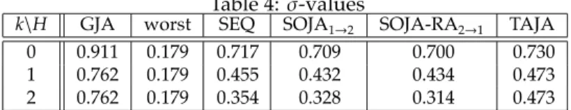
where k-nodes is the set of nodes in HRwith depth less or equal than k. Note that σ0(HR) is the utility value of the top-level partition in HRsince 0-nodes ={root}. The above measure allows us to valuate how well the local optimization objective is fulfilled. Table 4 gives σkvalues according to every approach, with
k value ranging from 0 to 2.
Table 4: σ-values
k\H GJA worst SEQ SOJA1→2 SOJA-RA2→1 TAJA
0 0.911 0.179 0.717 0.709 0.700 0.730
1 0.762 0.179 0.455 0.432 0.434 0.473
2 0.762 0.179 0.354 0.328 0.314 0.473
Hworst is the hierarchy provided by GJA with choice of the worst (instead of the best) partition at each step on the process. According to the example described in Section 3.2, Hworsthas only two levels: one root level and one cells level.
This measure is semantically consistent. Indeed, it reaches its maximum and minimum values on HGJA and Hworst respectively. Thus, we will use it to evaluate the validity of our joining processes (Section 6).
6 Experimental Results
This section presents experimental results achieved with the SOJA, SOJA-RA and TAJA processes. We first introduce the data set, then we provide an analysis based on observations of various parameters.
6.1 Data Set
We used a data set generator (DatGen4) to generate synthetic data sets with
different number of records. Each record is defined over N = 20 attributes with values from a set of 10 nominal values and has a primary key ID. To perform our joining processes, we previously computed two couples of hierarchies using the summarization service (without any mapping). The first set contains couples (G1, G2) such that D = RG1 "ID RG2 maps 200, 400, ..., 4000 cells and
G1 summarizes D over the first 2 attributes, whereas G2 summarizes it over
the remaining features. Thus, the number of cells of G2 that would join with
each cell of G1 is high. Let D& be a set of tuples that maps 10000 cells. The
second set contains couples (H1, H2) such that H1summarizes D&over the first
N1attributes, whereas H2summarizes D&over the last N− N1attributes, where
N1 ranges from 1 to 19. For each couple (G1, G2) (resp. , (H1, H2)), Gjoin (resp. ,
Hjoin) is the result of joining G1(resp. , H1) and G2(resp. , H2). For every couple
(G1, G2) (resp. (H1, H2)) we also process the join of RG1 (resp. , RH1) and RG2
(resp. , RH2) to provide the hierarchy GSEQ (resp. , HSEQ) with the centralized
approach.
All experiments were done on a 2.0GHz P4-based computer with 768MB memory.
6.2 Results
In this section, we validate our joining processes concerning performance (com-putation times), structural properties (number of nodes and leaves, average depth and average width) and σkmeasure.
6.2.1 Quantitative Analysis
From the analysis of theoretical complexities, we claim that TAJA, SOJA1→2and SOJA-RA1→2are much faster than the SEQ process performed on RG1 " RG2.
That is the main result of Figure 10 that shows the performance evolution according to the number of cells populated by RG1 " RG2. Furthermore,
SOJA-RA1→2 and TAJA are much more efficient than SOJA1→2. This is due to the fact that N1
N << 1 and consequently there exist high correlations between
RG1 and RG2 records. Note that, in real life data set, correlations will be less
high.
As one can observe, the SOJA-RA1→2 and TAJA are linear (i.e. , O(L)) in number of cells L of the joined hierarchy whereas SOJA1→2and SEQ are quasi-linear (i.e. , O(L· log(L))).
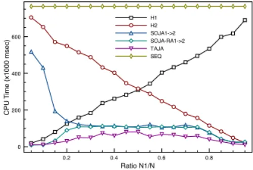
In this experiment (Figure 11), we use the second set of couples (i.e. , (H1, H2)) to show how CPU time of every joining process varies with changing
0 1000 2000 3000 4000 Number Of Cells 0.0 2.0 4.0 6.0 8.0 10.0 CPU T ime (x1000 msec) SEQ SOJA1->2 SOJA-RA1->2 TAJA y=x*ln(x) y=x
Figure 10: Time cost comparison - (G1, G2)
the fragmentation rate (N1
N). Observe that TAJA is a bit more efficient than SOJA-RA1→2. Further, as expected, the time cost of SOJA1→2is quite similar to that of SOJA-RA1→2, except for N1
N ≤ 0.20 since high correlations exist then between H1and H2(the base model H1is very small compared to H2).
0.2 0.4 0.6 0.8 Ratio N1/N 0 200 400 600 CPU T ime (x1000 msec) H1 H2 SOJA1->2 SOJA-RA1->2 TAJA SEQ
Figure 11: Time cost comparison - (H1, H2)
Thus, the joining processes are able to drastically reduce the time cost of the summarization task of a very large data set. This is achieved by vertical fragmentation into several sub-relations that would be summarized separately and then joined.
6.2.2 Qualitative Analysis
In the following, the average depth, average width and σkmeasure of joined hierarchies are reported, according to the fragmentation rate (N1
N).
As expected, Figure 12 shows that the average depths of the joined hier-archies of H1 and H2 provided by SOJA1→2and SOJA-RA1→2are greater than
that of the hierarchy provided by SEQ. The latter is also deeper than the one provided by TAJA.
In Figure 13, we can observe that hierarchies provided by TAJA are wider than those generated with SEQ. However, hierarchies provided by SEQ are wider than those provided by SOJA1→2and SOJA-RA1→2.
0.2 0.4 0.6 0.8 Ratio N1/N 6 8 10 12 14 16 18 A vg. Depth H1 H2 SOJA1->2 SOJA-RA1->2 TAJA SEQ
Figure 12: Average depth comparison
0.2 0.4 0.6 0.8 Ratio N1/N 2 2.2 2.4 2.6 2.8 3 3.2 3.4 3.6 3.8 A vg. Width H1 H2 SOJA1->2 SOJA-RA1->2 TAJA SEQ
Figure 13: Average width comparison
We can also see that the number of nodes is quite similar for SOJA1→2, SOJA-RA1→2 and SEQ hierarchies and is greater than that of the hierarchy provided by TAJA.
Note that for N1
N ≥ 0.30, H1 and hierarchies provided by SOJA1→2 and SOJA-RA1→2are the same from a structure point of view (i.e. , they have the same average depth, average width and number of nodes) since each cell of the base model H1is joined with exactly 1 cell of H2.
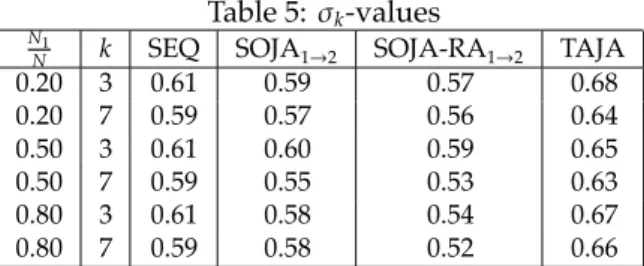
Finally, observe that σk values (Table 5) of the hierarchies provided by SOJA1→2 and SOJA-RA1→2 are in the same order of magnitude than that of hierarchies provided by the centralized approach. Furthermore, σk values of hierarchies provided by TAJA is greater than that of the hierarchies produced by SEQ. This is due to the fact that SEQ as well as many existing incremen-tal clustering algorithms suffer from ordering effects. The initial objects in an ordering establish initial clusters that "attract" the remaining objects and consequently, the quality of the generated clustering depends heavily on the initial choice of those clusters. This problem becomes more acute in the case of high dimensional data sets since it is common for all of the objects to be nearly equidistant from each other, completely masking well-defined starting clusters. However, TAJA joins well-defined clusters (from diverse areas of the object-description space) since the dimensionality of the data is reduced. Thus, each cluster of a joined partition is populated by objects that are close to each other and consequently, more similar on the full set of their attributes. On the
other hand, objects belonging to different clusters of a joined partition are well separated regarding the full space since they are highly separated regarding the two subspaces.
Table 5: σk-values N1
N k SEQ SOJA1→2 SOJA-RA1→2 TAJA
0.20 3 0.61 0.59 0.57 0.68 0.20 7 0.59 0.57 0.56 0.64 0.50 3 0.61 0.60 0.59 0.65 0.50 7 0.59 0.55 0.53 0.63 0.80 3 0.61 0.58 0.54 0.67 0.80 7 0.59 0.58 0.52 0.66
This analysis allows us to conclude that SOJA, SOJA-RA and TAJA provide well-founded summary trees.
Thus, those experimental results validate the theoretical hypotheses that our joining algorithms are very efficient, produce hierarchies with almost the same structural properties and achieve high quality results.
7 Related work
Extracting useful knowledge from large, distributed data is a very difficult task when such data cannot be directly centralized or unified as a single file or database due to a variety of constraints. So a new field called Distributed Knowledge Discovery (DKD) has emerged to handle the problem [16]. A com-mon classification of DKD algorithms in the literature separates them depend-ing on the nature of the data: homogeneously distributed data (horizontally partitioned) or heterogeneously distributed data (vertically partitioned).
There exist many different distributed clustering algorithms for analyzing data from homogeneous sites using different clustering notions, e.g. distribu-tion (or model) based [13, 7], density based [9, 12] or grid based [2]. However, our proposal is focused on vertically distributed data.
The problem of analyzing heterogeneously distributed data has been in-vestigated in many previous works. In [11], the authors develop a collective principal components analysis (PCA)-based clustering technique for vertically distributed data. Works in [21, 6, 17] report methods for combining cluster-ings in a centralized setting without accessing the features or algorithms that determined these partitions. Thus, these approaches can be adapted to hetero-geneously distributed data. In contrast to our proposal, the above approaches do not offer a solution to the distributed hierarchical clustering problem; they are based on partitioning techniques and generate a flat clustering of the data. Johnson and Kargupta propose in [10] a tree clustering approach to build a global dendrogram from individual dendrograms that are computed at local data sites. The algorithm first computes the element-wise intersection of all the most specialized clusters of sites to provide the most specialized partition of the whole data set, and then applies a single link clustering algorithm to compute the global dendrogram. This approach is similar to our SEQ-JA algorithm, but is less efficient since it is based on an agglomerative hierarchical clustering method. Indeed, its computational cost is O(n2), whereas for SEQ-JA it is
O(n· log n) where n is the size of the entire data set. In [4] (respectively [5]),
authors address decision tree (respectively bayesian network) learning from distributed heterogenous data. Both [4, 5] approaches are based on basic directed acyclic graph properties (the inner node specifies some test on a single attribute, the leaf node indicates the class, and the arc encodes conditional independencies between attributes). Since SEQ summaries are multidimensional and
unordered trees, such algorithms cannot be used to join them.
As far as we know, there are no multidimensional grid-based clustering algorithms for analyzing data from heterogeneous sites.
8 Conclusions
In this communication, we propose new algorithms for joining summary hier-archies obtained from two sets of database records with disjoint schemas. The
Subspace-Oriented Join Algorithm assumes one of the two input trees as the base
model and the other one is processed to complete the first one, whereas Tree
Alignement-based Join Algorithm rearranges summaries by levels in a top-down
manner. We show that SOJA, SOJA-RA and TAJA processes provide a good-quality joined hierarchy while being very efficient in terms of computational time.
As future work, we plan to generalize the proposed approaches to deal with overlapping schemas of different hierarchies, especially those that are se-mantically heterogeneous (with different fuzzy partitions) on their overlapping attributes.
References
[1] Rakesh Agrawal, Johannes Gehrke, Dimitrios Gunopulos, and Prabhakar Raghavan. Automatic subspace clustering of high dimensional data for data mining applications. SIGMOD Rec., 27(2):94–105, 1998.
[2] Mounir Bechchi, Guillaume Raschia, and Noureddine Mouaddib. Merg-ing distributed database summaries. In CIKM ’07, pages 419–428, Lisbon, Portugal, 2007.
[3] Indrajit Bhattacharya, Lise Getoor, and Louis Licamele. Query-time entity resolution. In KDD ’06, pages 529–534, New York, NY, USA, 2006. [4] D. Caragea, A. Silvescu, and V. Honavar. Decision tree induction from
distributed heterogeneous autonomous data sources, 2003.
[5] R. Chen, K. Sivakumar, and H. Kargupta. Collective mining of bayesian networks from distributed heterogeneous data. Knowl. Inf. Syst., 6(2):164– 187, 2004.
[6] Ana L. N. Fred. Data clustering using evidence accumulation. In ICPR
’02, page 40276, Washington, DC, USA, 2002.
[7] Joydeep Ghosh and Srujana Merugu. Distributed clustering with limited knowledge sharing, 2003.
[8] Maria Halkidi, Yannis Batistakis, and Michalis Vazirgiannis. On clustering validation techniques. Journal of Intelligent Information Systems, 17(2-3):107– 145, 2001.
[9] Eshref Januzaj, Hans-Peter Kriegel, and Martin Pfeifle. Towards effective and efficient distributed clustering, 2003.
[10] Erik L. Johnson and Hillol Kargupta. Collective, hierarchical clustering from distributed, heterogeneous data. In Large-Scale Parallel Data Mining, pages 221–244, 1999.
[11] Hillol Kargupta, Weiyun Huang, Krishnamoorthy Sivakumar, and Erik Johnson. Distributed clustering using collective principal component anal-ysis. Knowl. Inf. Syst., 3(4):422–448, 2001.
[12] M. Klusch, S. Lodi, and G. Moro. Distributed clustering based on sampling local density estimates, 2003.
[13] Hans-Peter Kriegel, Peer Kroger, Alexey Pryakhin, and Matthias Schubert. Effective and efficient distributed model-based clustering. In ICDM ’05:
Proceedings of the Fifth IEEE International Conference on Data Mining, pages
258–265, Washington, DC, USA, 2005.
[14] L.A.Zadeh. Concept of a linguistic variable and its application to approx-imate reasoning. Information and Systems, 1:119–249, 1975.
[15] L.A.Zadeh. Fuzzy sets as a basis for a theory of possibility. Fuzzy Sets and
Systems, 100:9–34, 1999.
[16] Kun Liu, Hillol Kargupta, Jessica Ryan, and Kanishka Bhaduri. Distributed data mining bibliography, 2004.
[17] N. NICOLOYANNIS P. E. JOUVE. A new method for combining partitions, applications for distributed clustering, 2003.
[18] E. Rosch and C.B. Mervis. Family ressemblances: studies in the internal structure of categories. Cognitive Psychology, 7:573–605, 1975.
[19] Regis Saint-Paul, Guillaume Raschia, and Noureddine Mouaddib. General purpose database summarization. In VLDB ’05, pages 733–744, 2005. [20] Parag Singla and Pedro Domingos. Entity resolution with markov logic.
In ICDM ’06, pages 572–582, Washington, DC, USA, 2006.
[21] Alexander Strehl and Joydeep Ghosh. Cluster ensembles: a knowledge reuse framework for combining partitionings. In Eighteenth national
con-ference on Artificial intelligence, pages 93–98, Menlo Park, CA, USA, 2002.
[22] K. Thompson and P. Langley. Concept formation in structured domains. In
Concept formation: Knowledge and experience in unsupervised learning, pages
127–161. Kaufmann, San Mateo, CA, 1991.
[24] Wei Wang, Jiong Yang, and Richard R. Muntz. STING: A statistical infor-mation grid approach to spatial data mining. In Twenty-Third International
Conference on Very Large Data Bases, pages 186–195, Athens, Greece, 1997.
Morgan Kaufmann.
[25] L. A. Zadeh. Fuzzy sets. Information and Control, 8:338–353, 1965.
Contents
1 Introduction 3
2 Overview of the SEQ System 4
2.1 A Two-Step Process . . . 4
2.1.1 Mapping Service (MSEQ) . . . 4
2.1.2 Summarization Service (CSEQ) . . . 5
2.2 Features of the Summaries . . . 6
2.3 Time complexity of SEQ . . . 7
2.4 The General Case . . . 8
3 Problem Analysis 9 3.1 Problem Statement . . . 9
3.2 Running Example . . . 10
3.3 Basic Approaches . . . 11
4 Alternative approaches 14 4.1 Subspace-Oriented Join Algorithm . . . 14
4.2 SOJA with Rearrangements . . . 15
4.3 Tree Alignement-based Join Algorithm . . . 17
5 Joining validity assessment 18 5.1 Background . . . 18
5.2 Summary Tree Quality . . . 19
6 Experimental Results 20 6.1 Data Set . . . 20 6.2 Results . . . 20 6.2.1 Quantitative Analysis . . . 20 6.2.2 Qualitative Analysis . . . 21 7 Related work 23 8 Conclusions 24
Centre de recherche INRIA Bordeaux – Sud Ouest : Domaine Universitaire - 351, cours de la Libération - 33405 Talence Cedex Centre de recherche INRIA Grenoble – Rhône-Alpes : 655, avenue de l’Europe - 38334 Montbonnot Saint-Ismier Centre de recherche INRIA Lille – Nord Europe : Parc Scientifique de la Haute Borne - 40, avenue Halley - 59650 Villeneuve d’Ascq
Centre de recherche INRIA Nancy – Grand Est : LORIA, Technopôle de Nancy-Brabois - Campus scientifique 615, rue du Jardin Botanique - BP 101 - 54602 Villers-lès-Nancy Cedex
Centre de recherche INRIA Paris – Rocquencourt : Domaine de Voluceau - Rocquencourt - BP 105 - 78153 Le Chesnay Cedex Centre de recherche INRIA Saclay – Île-de-France : Parc Orsay Université - ZAC des Vignes : 4, rue Jacques Monod - 91893 Orsay Cedex
Centre de recherche INRIA Sophia Antipolis – Méditerranée : 2004, route des Lucioles - BP 93 - 06902 Sophia Antipolis Cedex
Éditeur
INRIA - Domaine de Voluceau - Rocquencourt, BP 105 - 78153 Le Chesnay Cedex (France) http://www.inria.fr