Building and HVAC optimal control simulation. Application to an office building.

BUILDING AND HVAC OPTIMAL CONTROL SIMULATION.

APPLICATION TO AN OFFICE BUILDING

Michaël KUMMERT, Philippe ANDRÉ and Jacques NICOLAS

Fondation Universitaire Luxembourgeoise

Avenue de Longwy, 185 B 6700 Arlon (BELGIUM)

[email protected]

ABSTRACT

This paper describes the methodology to apply discrete-time optimal control to a building and its HVAC installation. Simulation-based results concerning a passive solar commercial building are presented and discussed. The simulation environment includes the TRNSYS TYPE 56 as reference building model and HVAC detailed models to test the controller with realistic control signals. The optimal controller's sensitivity to meteorological forecasting quality and to other factors is analysed. Its performance is compared to results obtained with a conventional control system to assess the relevancy of optimal control for this application.

1.

INTRODUCTION

Modern office buildings are often characterised by a high level of internal gains due to intensive use of electrical appliances. In the case of passive solar buildings, but also for many recently designed buildings, important solar gains contribute as well to lessen the heating load already reduced by a good thermal insulation.

The share of heating cost in the total operation cost of this type of building is usually very low and heating control is probably not the main concern of building owners or maintenance companies. However, energy savings can still be realised by a better control strategy. Furthermore, this high level of uncontrolled gains can lead to uncomfortable overheating periods, even during the heating season. A "smart" heating control strategy should take both concerns into account in order to minimise occupants discomfort while keeping the energy consumption as low as possible.

The "Energy, Environment and sustainable development" work programme of the EC Fifth Framework Programme (European Commission, 1999) mentions improved Building Energy Management Systems as a mean to reduce energy consumption. This document highlights that "The target for Building Energy Management Systems is to reduce the energy consumption by 7% in 2010, while responding to user needs and climate variations."

Optimal control theory is well suited for this twofold objective, as its principle is to anticipate the system evolution to minimise a cost function which can easily include a comfort-related term and an energy-related one.

Optimal control of auxiliary heating plant in solar buildings was considered by different authors in the eighties (Winn & Winn, 1985 and Rosset & Benard, 1986). These papers present simulation-based results using simple models for the building and HVAC plant. They show that substantial energy savings and comfort improvement can be achieved. Later, André (1992) and Fulcheri et al. (1994) showed that these gains were significantly reduced when they were evaluated on more complex models and a fortiori on real buildings, if the internal model of the controller was too simple.

Interest for optimal control rised again in the nineties, mainly for cooling applications. Braun (1990) considered an entire cooling plant and one building zone, to study the possible energy and cost

savings of optimal control compared to conventional night set-up control. The optimisation of the cooling plant was achieved using a steady state performance map obtained with detailed models, and was de-coupled from the building dynamic analysis. A parametric study covering a wide range of conditions was made with synthetic weather data and considering "steady periodic" solutions. Keeney and Braun (1996) showed that a large fraction of these energy cost savings could be obtained with a simplified control strategy. The optimisation of two control variables (e.g. pre-cooling period and power), combined with a classical comfort-based controller with simple rules during building occupancy, can yield about 95% of possible energy savings using optimal control. This solution drastically reduces the computational load of the optimisation.

In cooling applications, achievable cost savings are rather impressive, taking advantage of the time-of-day electricity rate (off-peak rate can be 1/3 from on-peak rate). The real energy consumption is only slightly reduced, or even increased. In the case of non-electrical heating, achievable cost savings are less impressive but they are always combined with real energy savings. This paper shows that thermal comfort can be improved while reducing the energy consumption, compared with a classical controller, which makes optimal control doubly interesting.

2.

CONSIDERED SYSTEM

The system (Fig 1) includes a part of the building and the heating installation. The considered building part consists of two thermal zones of a passive solar commercial building: two offices (30 m²) and an adjacent south facing sunspace. The sunspace is 1 m deep and totally glazed. It is separated from the offices by a mass wall (heavy concrete, 25 cm) including 10 m² internal windows. External windows (2m²),which can be opened by occupants, are also present in offices. The hot water heating system includes a boiler, a three-way valve and a radiator. The control variable is the water supply temperature, Tws. In the reference case, a

thermostatic valve is present on the radiator. This valve is supposed to be fully opened in the case of optimal control. The controlled variable is the operative zone temperature in offices (Top).

3.

OPTIMAL CONTROL ALGORITHM

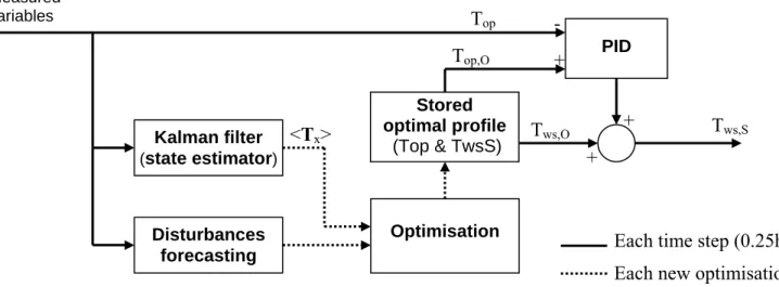
Fig. 2 represents the block-scheme of the optimal controller. The principle is briefly described here under, while next sections give some details on the different blocks.

1.At each time step (0.25h) some variables are measured : zone operative temperature (Top),

radiator supply and exhaust temperature (resp. Tws and Twe), ambient temperature (Tamb) and

solar radiation on southern facade (GS).

2.These variables are passed to a Kalman Filter, which estimates the state of the simplified model included in the optimal controller (<Tx>), and to a disturbances forecasting algorithm

which predicts the ambient temperature and solar radiation for the next optimisation period (e.g. 24h).

3.At each beginning of a new optimisation period, the optimisation algorithm minimises the cost function on the optimisation horizon (NH), giving a 0.25h-profile of Top and Tws (respectively

Top,O and Tws,O). It uses the estimated state of the system and the disturbances forecasting.

4.A PID controller tracks the setpoint for Top (Top,O), correcting the optimal water supply

temperature (Tws,O) to give finally the setpoint for Tws to the heating plant (Tws,S).

Fig 1: simulated system

radiator

Offices

boiler Tws

Fig. 2 : Optimal controller block scheme 3.1. Simplified model

The linear state-space building model, based on a second-order wall representation, was developed for control purposes and is presented in an earlier paper (Kummert et al., 1996). It has been optimised to realise a compromise between accuracy and complexity.

The radiator is modelled as a single node and heat emission characteristics are linearised. The average temperature between radiator (TR) and water supply (Tws) is used to compute the power

emission. Heat flux is directed to air and to wall surfaces according to a fixed ratio. The radiator equation is written as:

(

ws R

)

w ws R ms r , R ws R a c , R R R C T T 2 T T T UA 2 T T T UA d dT C + −      ₋ + +       ₋ + = τ & (1) with

CR : radiator thermal capacity [J/K]

UAR,r ; UAR,c : radiator radiative and convective heat exchange coefficients [W/K]

TR : radiator temperature, considered equal to water return temperature (Twe) [°C] Ta, Tms : resp. air and mean surface temperature of the zone [°C]

Tws : water supply temperature [°C]

w

C& : water capacitive flow rate [W/K] 3.2. State estimator

The model initial state must be estimated at the beginning of each optimisation period. This is realised by a Kalman filter using the measured zone temperature (Top) and measured inputs and disturbances: radiator supply and return water temperature (resp. Tws and Twe), ambient conditions (GS and Tamb).

3.3. Cost function

Controllers will be evaluated using a cost function, which express their global performance. This cost function must be an expression of the trade-off between comfort and energy consumption. The

<Tx> Measured variables Disturbances forecasting Optimisation Kalman filter (state estimator) Stored optimal profile (Top & TwsS) PID Top,O Tws,O Top + + + - Tws,S

Each time step (0.25h) Each new optimisation

chosen indicator of thermal comfort is Fanger's PPD (Fanger, 1972), while energy cost is considered to be proportional to the boiler energy

consumption (Qb).

In the discomfort cost, PPD is computed with default parameters for non-simulated aspects (air velocity, humidity and metabolic activity). Furthermore, it is assumed that occupants can adapt their clothing to the zone temperature. This method allows modelling a comfort range in which occupants are satisfied. With the chosen value for parameters, the comfort zone covers operative temperatures from 21°C to 24°C. PPD is also shifted down by 5%, to give a minimum value of 0. This modified PPD index will be referred to as PPD'. Discomfort cost is represented Fig.3.

This gives, respectively for discomfort cost and energy cost (Jd and Je):

(

)

∫

− = PPD[%] 5 J_d (2)

∫

= b e Q J & (3)

The global cost (J) is a weighted combination of both:

e

d J

J

J=α + (4)

The principle of minimising a cost function is the basis of optimal control theory. It seems natural to use the same cost function in the controller than the one that will be use to evaluate its performance afterwards. The cost function implemented in the controller is a quadratic-linear function, where the quadratic term is an approximation of PPD' and the linear term is exactly Je. It is detailed in an

earlier paper (Kummert et al., 1997). 3.4. Disturbances forecasting

Internal gains are related to occupancy schedules, which are well known in office buildings. A forecasting routine is currently under development for meteorological disturbances. This routine will use local measurements and global forecasting from a meteo server to predict hourly profiles of temperature and solar radiation. Two extreme solutions were adopted in this study: perfect forecasting and use of the previous day. A third forecasting method considering a mean day was also considered in the evaluation of the forecasting quality on the controller performance in sec. 6.3. 3.5. Optimisation algorithm

The problem of finding the control sequence minimising a linear-quadratic cost function for the given linear system can be rewritten as a quadratic-programming problem (Kummert et al., 1997). This guarantees the existence of a solution and allows the use of efficient projected gradient algorithm. This algorithm was implemented in Matlab Optimisation Toolbox, which was used for the optimal control computation (Grace, 1996). The system includes 11 state variables. For a 24 steps-ahead optimisation, the total number of variables in the QP-problem is 325, and 397 linear constraints are necessary. Typical computational time is about 40 sec on a Pentium II - 350 PC,

Fig. 3 : Discomfort Cost

15 20 25 30 0 5 10 15 20 25 30 35 40 45 50 Top [°C] J d

using Matlab (a C++ equivalent code should run much faster). Memory requirements are not too high since most matrices are sparse.

In the case of perfect modelling and perfect disturbances forecasting, the optimisation should be repeated only at the end of the period on which the cost function was minimised. However, to reduce the influence of modelling and forecasting errors, a "receding horizon" is used, i.e. the optimisation is repeated with a period smaller than the prediction horizon. The prediction horizon and the time step for new optimisation will respectively be referred to as NH and NC. Both are

expressed in [h].

In this study, optimisation horizons (NH) ranging from 12 to 24 h were considered, and this

optimisation was repeated up to every 6 hours (NC range : 6..12h). In the case of a 24h-ahead

prediction repeated every 6 h, for example, only the first six values of optimal control signals are applied.

3.6. PID controller

When a new optimisation is computed, a feedback from the real system is present, since the estimated state of the system based on measured outputs is used. During the period between two optimisations, the computed optimal control profile is applied without any feedback from the real system. In the case of large forecasting errors, this can lead to a system evolution being far from the predicted one and hence far from "the optimum". To compensate for these errors, a feedback controller is cascaded with the optimisation. This controller is a conventional PID with anti-windup and uses the base time step (0.25h).

4.

IMPLEMENTATION IN A SIMULATION ENVIRONMENT

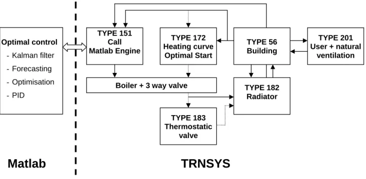
The role of the real system is played by different models implemented in the TRNSYS software. The conventional controller (heating curve + optimal start) is also a TRNSYS routine, while the optimal controller is implemented in Matlab. The communication between TRNSYS and Matlab is realised by a special TRNSYS TYPE calling the Matlab Engine Library (Kummert and André, 1999). The simulation scheme is represented by Fig. 4.

Fig. 4. Simulation scheme

TYPE 182 Radiator TYPE 151 Call Matlab Engine TYPE 172 Heating curve Optimal Start TYPE 56 Building TYPE 201 User + natural ventilation

Boiler + 3 way valve Optimal control - Kalman filter - Forecasting - Optimisation - PID TYPE 183 Thermostatic valve

TRNSYS

Matlab

The simulation time step is 0.25h.

The building is simulated by TRNSYS TYPE 56. It solves a detailed heat balance of the building, using the z-transform method to evaluate the conductive heat fluxes through walls. A single output is considered in the simulation: the operative temperature in offices zone.

The building has windows that can be opened by occupants. To take this possibility into account, a rough model of the user behaviour and natural ventilation was developed (TYPE 201). The user is supposed to open windows when the temperature rises above the maximum comfort temperature (24°C). She/he is supposed to close them when the temperature falls below the lower comfort bound (21°C). The natural ventilation is modelled by a variable infiltration rate in TYPE 56. The infiltration rate is estimated by a regression on wind speed and direction. This variable infiltration rate is not taken into account in the optimal controller, which is not supposed to know the user behaviour in this respect.

The radiator and thermostatic valve models (TYPE's 182 and 183) are based on IEA Annex 10 models (IEA, 1988). Non-linear characteristic is conserved for the radiator power, but the discrete-time equation is solved in a new way, which is suitable for longer discrete-time steps (0.25h). The thermostatic valve is supposed to be fully opened when optimal control is applied.

The boiler and the three-way valve are simply modelled by "TRNSYS equations". The water supply temperature is computed from the desired value (setpoint from the controller), taking into account bounds coming from the water return temperature and boiler maximum power.

The controller is either a conventional one (TYPE 172, Heating curve and optimal start) or the optimal controller called by TYPE 151. The conventional controller is described in section 5.2.

5.

SIMULATION TESTS

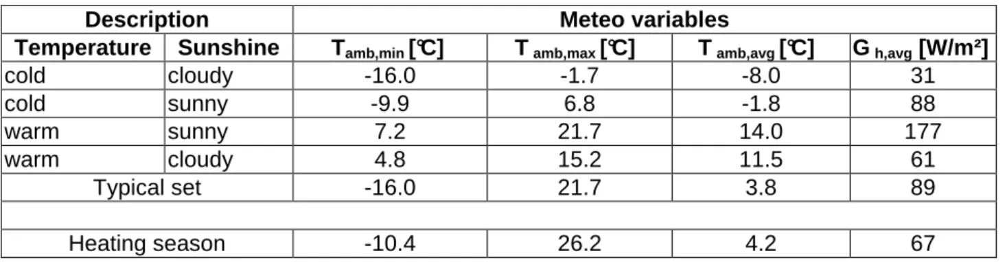
The passive solar commercial building described in section 2 was implemented in the simulation environment and several simulations were realised using both controllers (conventional and optimal) with different parameters. All simulations were realised with real measured meteo data from Uccle (Brussels), in the years 1985-1986.

5.1. Meteo Data

First, a "typical meteo set" for heating period was constructed. This data set contains four typical weeks concatenated. It served to test different settings of the optimal controller and to study its behaviour in more details.

In a second phase, a whole heating season (30 weeks) was used, to assess the optimal controller performance and to compare it with the conventional controller. Data sets characteristics are presented Table 1. (Gh is the global horizontal solar radiation)

Table 1 : Meteo data sets

Description Meteo variables

Temperature Sunshine Tamb,min [°C] Tamb,max [°C] Tamb,avg [°C] Gh,avg [W/m²]

cold cloudy -16.0 -1.7 -8.0 31 cold sunny -9.9 6.8 -1.8 88 warm sunny 7.2 21.7 14.0 177 warm cloudy 4.8 15.2 11.5 61 Typical set -16.0 21.7 3.8 89 Heating season -10.4 26.2 4.2 67

5.2. Conventional controller

Traditional heating control strategies include a feed-forward action on water supply temperature by the so-called "heating curve" and a feedback action on water flow rate by a thermostatic valve. Moreover, up-to-date controllers use an optimal start algorithm. Our reference control strategy combines these three features.

The heating curve consists actually of two different curves, giving the required water supply temperature to maintain desired setpoints (night and day) in the reference zone. In this case, setpoints were fixed to 15°C (night) and 21°C (day). Furthermore, the "day" heating curve is slightly over-estimated to take into account the dynamic evolution of the building. Indeed, these curves are calculated in steady-state regime, which is never the case in practice. The building structure is always colder than in the corresponding steady-state, since a night set-back is applied. The thermostatic valve has a dead band of 2°C, and different settings of the thermostat are compared.

The optimal start algorithm uses a non-linear function proposed by Hittle and O'Connor (cit. in Seem et al., 1989) to estimate the recovery time from night set-back. This relation uses the current temperature of the zone, the ambient temperature, and the desired final temperature. Parameters for this building were identified by a regression using TRNSYS simulation results. Two different parameters sets were kept (the second one gives a more conservative estimate of the return time) Different conventional solutions are referred to as 'Cc' for the conservative parameter set, and 'Cr' for the "risky" one.

6.

RESULTS

6.1. Comfort/Energy trade-off

The cost function implemented in the optimal controller is presented in eq. (2), (3) and (4). α is a parameter which allows to give more or less importance to comfort versus energy consumption. As above-mentioned, the discomfort cost (Jd) implemented in the controller is an approximation of

PPD' (PPD shifted to give a minimum of 0 and not 5% and computed with variable clothing). This value is integrated and can be expressed in [%h]. If we express the energy cost (Je) in kWh, α units

are [kWh/%h]. α can thus be interpreted as "the energy quantity (expressed in kWh) that we accept to consume to reduce the percentage of dissatisfied people in the building by 1% during 1h". Despite this fact, the ratio between total energy consumption and integrated value of PPD' on a long period will not be equal to α. This is illustrated in Table 2 and Fig. 5, which compare the total energy consumption and integrated PPD for the typical meteo data set, and for different α values in the range [1;10].

Table 2: Je and Jd for different α values α αα α [kWh/%h] Je/Jd [kWh/%h] Je [kWh] Jd [%(PPD') h] 10 68.8 550 8 5 62.0 539 8.7 4 54.2 537 9.9 3 39.2 533 13.6 2 22.3 526 23.6 1 7.9 511 65 0.0 20.0 40.0 60.0 80.0 0 2 4 6 8 10 α α α α [kWh/%] J e /J d [k W h /% ]

It is clear that α is linked to Je/Jd, but the value of this ratio on a long period (e.g. one heating season) is not easily predictable. The relation between these two variables is even not linear: a "saturation" happens for high α values, when the upper limit of comfort achievable with the heating plant is reached. Furthermore, the curve is different if other controller settings are changed (e.g. NH and NC).

6.2. Optimisation horizon and "new computation" time step

Every NC hours, a new optimisation is computed, minimising the cost function on NH hours. This

implies that only the first NC optimised setpoints are applied. This principle, known as "receding

horizon", is commonly applied in predictive control.

The selection of NH and NC depends on the building and on the model and forecasting quality. NH

must be long enough to allow an effective anticipation of disturbances. This means for example that NH must be larger than the recovery time from night set-back in the worst case. It should be

possible as well to under-heat the building during the morning in the case of afternoon overheating. This requires to reduce heating before 7 AM because of an overheating which can occur after 4PM case, which implies a NH value greater than 9 hours.

We tested different values for NH (24;20;18;16;12;8) and NC (24;12;8;6). In the case of perfect

weather forecasting, no difference was noted between different NC values smaller than 12h.

Relatively small modelling errors can explain this: linearisation of the radiator power, reduced order of wall models and constant infiltration rate. When imperfect forecasting was used, NC values larger

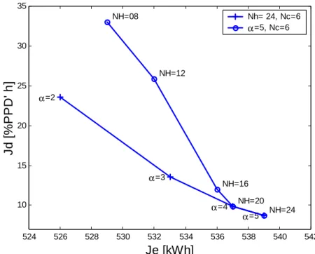
than 8 hours give a poor behaviour of the optimal controller, 6 hours giving even better results. Fig. 6 shows the decrease in

controller performance caused by a reduction of the optimisation horizon, for a constant NC value of 6h (α = 5

kWh/%h). This plot represents Jd versus Je. The closer a controller is to the lower left corner, the better its performance is. The dotted line shows the trajectory followed by results when varying α for constant NH and NC. For

constant NC and α, when NH is

reduced, the trajectory is different and shows a poorer performance. NH values greater

than 18h seem to be suitable, but the performance of the controller decreases rapidly when NH falls below this value.

The difference may seem insignificant (e.g. for a similar discomfort of 20, the increase in energy consumption is about 1%), but the comparison with a conventional controller must be taken into consideration. If savings of the optimal controller are 5%, this 1% absolute loss represents 20% of possible savings. 524 526 528 530 532 534 536 538 540 542 10 15 20 25 30 35 α=5 α=4 α=3 α=2 NH=24 NH=20 NH=16 NH=12 NH=08 J d [ % P P D ' h ] Je [kWh] Nh= 24, Nc=6 α=5, Nc=6

6.3. Forecasting quality

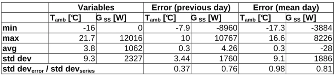
Three meteo forecasting types were investigated for the typical meteo data set: Perfect forecasting, use of the previous day and use of a "mean day". The latter is constructed by averaging all days on a hour-by-hour basis. This forecasting is of poorer quality, as shown in Table 3. This table presents statistics on two relevant variables: the ambient temperature (Tamb) and the total solar radiation

entering the sunspace (GSS). Statistics on forecasting errors show that the error standard deviation

reaches 80% of the variable standard deviation for GSS, and about 100% for Tamb

Table 3 : Forecasting error statistics

Variables Error (previous day) Error (mean day)

Tamb [°C] GSS [W] Tamb [°C] GSS [W] Tamb [°C] GSS [W]

min -16 0 -7.9 -8960 -17.3 -3884

max 21.7 12016 10 10767 16.6 8226

avg 3.8 1062 0.3 4.26 0.3 -28

std dev 9.3 2327 3.44 1760 9.1 1886

std deverror / std devseries 0.37 0.76 0.98 0.81

Fig. 7 shows the effect of forecasting errors on the controller performance. Different values of α are used (1 to 5) for each forecasting case. The performance decrease resulting from the use of "previous day" forecasting is not

too important: for a discomfort about 12, the energy consumption rises from 533 to 538, which represents a 1% increase. The difference increases for lower α values (higher part of the plot). This can be explained by the greater freedom left to the controller for small α values: achievable gains are more important in this case, but the optimal zone temperature profile is very dependent on meteo conditions. In this case, a forecasting error has a larger influence. The comparison with the conventional controller shows that the optimal controller still gives a better performance despite imperfect forecasting.

In the case of "mean day" forecasting, the controller performance is quite poor, and low discomfort cost values cannot be attained.

This comparison shows that the quality of meteo forecasting is an important factor for the controller. The use of the previous day seems to be a satisfying solution, which is rather surprising. This conclusion has to be confirmed on a longer data set (this graph concerns the "typical set", but next section will confirm these results for the whole heating season).

The PID plays a determinant role in the case of imperfect forecasting. Table 4 gives statistics on the PID action for the three forecasting types. Three variables are considered : Top, Tws and Q&b(zone

510 520 530 540 550 560 570 580 590 0 10 20 30 40 50 60 70 J d [ % P P D ' h ] Je [kWh] Optimal - Perfect Optimal - Previous day Optimal - Mean day Conventional

temperature, water supply temperature and boiler power). First, the mean value and standard deviation are presented for each variable. For Top, the error between the desired value by the

optimal controller and the real value is analysed. For Tws and Q&b, the PID correction (between the

setpoint given by the optimisation itself and the final setpoint given to the three-way valve) is considered. Values given for Q&_bare estimated, since the real control signal is Tws (the controller

has no direct influence on Q&_b).

Table 4. PID action (entire Typical data set). Top and Tws are in °C, Q&_bin Wh

Perfect forecasting Previous day "Mean day"

Top Tws b Q& Top Tws b Q& Top Tws b Q& avg 19.5 36.1 830 19.5 36.2 831 19.5 36.1 833 std dev 2.5 25.2 1252 2.5 25.1 1249 2.6 25.3 1273 std dev of error 0.06 0.25 0.29

std dev of PID corr 2.84 171 6.30 336 9.00 469

The PID correction remains relatively small for the first case, but the results for imperfect forecasting show clearly that the PID is important.

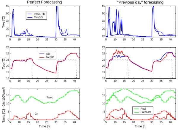
Fig. 8 illustrates the PID behaviour on two days for which the "previous day" forecasting was rather incorrect. It must be noted that the PID is bounded by some "common sense" rules. Tws is for

instance not corrected if Top is lower than the expectations but still higher than the lower comfort limit. This happens during the first day, when the expected sunshine is higher than real one. The PID is allowed to correct the temperature to 21.5°C, but not higher. Actually, a PID correction is only possible if the zone temperature is lower than the lower bound of the comfort zone and if the building is occupied or in the "morning pre-heating" phase. In all other cases, the PID can only decrease Tws. 5 10 15 20 25 30 35 40 20 30 40 50 60 T w s [ °C ] Perfect Forecasting TwsSPID TwsSO 5 10 15 20 25 30 35 40 18 19 20 21 22 23 T o p [ °C ] Top TopSO 5 10 15 20 25 30 35 40 0 5 10 15 Time [h] T a m b [ °C ] - G h [ 1 0 0 W /m ²] 5 10 15 20 25 30 35 40 20 30 40 50 60

"Previous day" forecasting

5 10 15 20 25 30 35 40 18 19 20 21 22 23 5 10 15 20 25 30 35 40 0 5 10 15 Time [h] Real Forecast Gh Tamb

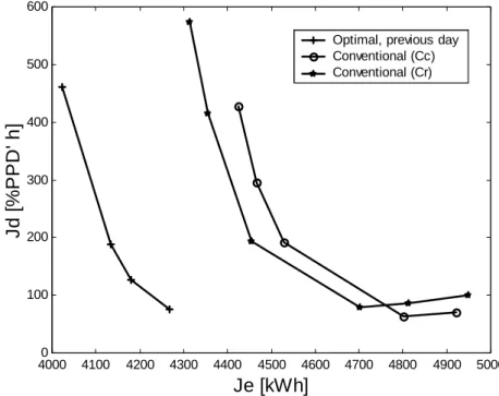
6.5. Comparison on an entire heating season

Fig. 9 uses the representation introduced in section 6.2. (Jd vs. Je) to compare optimal and conventional controllers.

As mentioned in section 5.2., two different parameter sets are used for the optimal start algorithm. They give the two curves labelled 'Cc' and 'Cr'. Different settings for the thermostatic valves explain the variations along these curves. For the optimal controller, previous day forecasting is used and different α values are compared.

Energy savings for a similar discomfort reach 7 to 9%, which is close to the performance obtained by Nygard-Fergusson (1990) for stochastic optimal control of floor-heated offices.

These results show that optimal control could be one solution to achieve EC's objective mentioned in the introduction, which is to reduce energy consumption by 7% in 2010 through improved BEMS.

7.

PRACTICAL ASPECTS

Simulation results show that optimal control can contribute to reduce building energy consumption, in conjunction with better design and retro-fitting of existing buildings. Depending on the size of the building, two options are possible:

Large buildings are often equipped with a BEMS and the implementation within this BEMS of the optimal control algorithm presented in this paper should be possible. Furthermore, most large buildings are equipped with needed sensors (except the solar radiation sensor, which is not common) and sometimes connected to meteo servers giving good quality weather forecasting. The "hardware" investment cost is rather small compared to heating cost and the payback time should be short.

For small buildings or even single family houses, implementation of the optimal control algorithm in a common micro-controller should be possible. Such micro-controllers are quite common, even if they are mostly used for simple scheduling of the heating curve. The computational load is quite high compared to classical control algorithms, but the needed time step is large (e.g. 0.25h). In this case, the investment represented by new sensors (especially solar radiation sensor) could be a limitation, but cheap PV sensors are currently introduced on the market and their price is expected to decrease rapidly. The payback time could be longer here, but environmental considerations could replace the financial incentive… The forecasting of building occupancy and internal gains could be less accurate and this may have a negative influence on the controller performance.

40000 4100 4200 4300 4400 4500 4600 4700 4800 4900 5000 100 200 300 400 500 600 J d [ % P P D ' h ] Je [kWh]

Optimal, previous day Conventional (Cc) Conventional (Cr)

8.

CONCLUSIONS

Simulation of the optimal control performance on realistic reference models has shown that the developed controller is able to efficiently control the room operative temperature and to maintain a good level of comfort. Furthermore, choice is given to building users to privilege either the comfort or energy savings thanks to a simple parameter. Comparisons with classical reference controllers showed that significant energy savings can be realised maintaining thermal comfort. Both comfort and energy savings can even be improved together in the case of "afternoon overheating". The use of a poor quality weather forecast (previous day) reduces the controller performance. However, the compensating PID and the use of a receding horizon seem to limit this effect, giving a global performance still better than the considered conventional controller. These results have been obtained on a passive solar commercial building presenting important overheating periods during the heating season. Further work will address the evaluation of the optimal controller’s performance on other buildings and the experimental validation of presented results. In this respect, the lack of on-line identification of the controller model seems to be the main limitation. This problem will be tackled in our future research.

REFERENCES

1. André Ph. et Nicolas J., 1992 - Application de la théorie des systèmes à la thermique du bâtiment. Problèmes de modélisation, d'identification, de contrôle. Revue Générale de Thermique, n°371, p. 600-615.

2. Braun J.E., 1990 - Reducing energy cost and peak electrical demand through optimal control of building thermal storage. ASHRAE Trans., vol. 96 (2).

3. European Commission, 1999 - Energy, environment and sustainable development. Programme for Research, Technology Development and Demonstration under the Fifth Framework Programme. Available on http://www.cordis.lu/fp5/src/t-4.htm

4. Fanger P.O., 1972 - Thermal comfort analysis and application in environmental design. Mac Graw Hill. 5. Fulcheri L., Neirac F.P., Le Mouel A. et Fabron C., 1994 - Chauffage des bâtiments. Intermittence et

lois de régulation en boucle ouverte. Revue Générale de Thermique, n°387, p. 181-189.

6. Grace A., 1996 - Optimisation toolbox for use with Matlab 5. The MathWorks Inc, Natick MA.

7. IEA, 1988 – Building and Community Systems (BCS) programme, Annex 10. System Simulation. Technical reports. International Energy Agency. http://www.ecbcs.org/annex10.html

8. Keeney K. and Braun J.E., 1996 - A simplified method for determining optimal cooling control strategies for thermal storage in building mass. HVAC&R Research, vol. 2 n°1.

9. Kummert M., André Ph. and Nicolas J., 1996 - Development of simplified models for solar buildings optimal control. Proc. ISES Eurosun 96 congress, Freiburg.

10. Kummert M., André Ph. and Nicolas J., 1997 - Optimised thermal zone controller for integration within a Building Energy Management System. Proc. CLIMA 2000 conf. (CD-ROM), Brussels.

11. Kummert M. and André Ph., 1999 – Coupling TRNSYS to Matlab through the "Matlab Engine Library". Application to building control simulation. TRNSYS club meeting, 22-23 March 1999. University of Liège, laboratory of Thermodynamics.

12. Nygard-Fergusson A.-M., 1990 - Predictive thermal control of building systems. Ph. D. Thesis, Ecole Polytechnique Fédérale de Lausanne.

13. Rosset M.M. et Benard C., 1986 - Optimisation de la conduite du chauffage d'appoint d'un habitat solaire à gain direct. Revue Générale de Thermique, vol. 291, p. 145-159.

14. Seem J.E., Armstrong P.R. and Hancock C.E., 1989 - Algorithms for predicting recovery time from night setback. ASHRAE Trans., vol. 95 (2), p. 439-446

15.Winn R.C. and Winn C.B., 1985 - Optimal control for auxiliary heating of passive-solar-heated buildings. Solar Energy, vol. 35, n°5, p. 419-427.