APPLICATIONS OF AN INTERIOR POINT METHOD BASED OPTIMAL POWER FLOW
Florin Capitanescu Mevludin Glavic Louis Wehenkel
Department of Electrical Engineering and Computer Science, University of Li`ege, Belgium
ABSTRACT
This paper tackles the complex problem of an optimal power flow (OPF) by the interior point method (IPM). Two interior point algorithms are presented and com-pared, namely the pure primal-dual and the predictor-corrector respectively. Among various OPF objectives, emphasis is put on two classical ones: the maximization of loadability limit and the minimization of the amount of load curtailment. Illustrative examples on three test systems ranging from 60 to 300 buses are provided.
1 INTRODUCTION
Since the early 60’s [1] the Optimal Power Flow (OPF) problem has become progressively an indispensable tool in power systems planning, operational planning and real-time operation, and that whatever the electricity mar-ket environment: liberalized or not [2].
The OPF is stated in its general form as a nonlinear, non-convex, large-scale, static optimization problem with both continuous and discrete variables. It aims at op-timizing some objective by acting on available control means while satisfying network power flow equations, physical and operational constraints. Among various OPF objectives, we focus on this paper on two classical ones: the maximization of power system loadability [12] and the minimization of amount of load shedding [11]. Both are very valuable piece of information for the trans-mission system operator (TSO).
The pre- and post-contingency loadability limit (and mar-gin) indicates how far the system is from voltage collapse or from violating some operating constraints (e.g. branch currents, bus voltage magnitudes). The simplest method for determining a loadability limit consists in repeated load flows, performed for increasing values of the system stress, until either divergence is met or some operating constraints are violated. Avoiding the uncertainty of load flow divergence, the continuation power flow [10] allows to trace the solution path passing through the loadability limit, while the quasi-steady state simulation evaluates the sought limit by a dynamic ramp stress increase [14]. Optimization methods, on the other hand, directly ob-tain the limit as the solution of an optimization problem whose objective is to maximize a system stress [12, 17]. Optimization methods have the advantage over the three other approaches that they can also maximize a loadabil-ity limit by optimally adjusting control means.
In an emergency situation (when following a load in-crease and/or a contingency the system losses its
equilib-rium point and/or some operating limits are significantly exceeded), the minimum amount of load shedding pin-points where and how much load to curtail in order to re-store either an equilibrium point of the system and/or to remove operational constraints violations [11]. Whereas the determination of minimal load shedding for removing thermal overloads or raise small voltages is rather simple as long as the system is voltage stable, it becomes a very challenging problem in a voltage unstable scenario [9]. Restoring system feasibility in a voltage unstable sce-nario may be tackled either by dynamic simulation [13] or by static optimization [11].
The Interior Point Method (IPM) [3] is the most fashion-able approach of the OPF problem due to its speed of convergence and ease handling of inequality constraints by logarithmic barrier functions [11, 12, 15].
In this paper we compare two interior point (IP) based algorithms, namely the pure dual and the primal-dual predictor-corrector, called for the sake of brevity in the remaining of the paper PD and PC respectively. The paper is organized as follows. The section 2 in-troduces the OPF problems. Section 3 offers a short overview of both PD and PC algorithms. Section 4 pro-vides some numerical results while some conclusion are drawn in Section 5.
2 OPTIMAL POWER FLOW FORMULATIONS 2.1 Maximum Loadability Problem
The loadability limits (and margins) considered in this paper rely on the definition of a system stress. The latter consists in changes in bus power injections which weaken the system by: increasing power transfers over relatively long distances, drawing on reactive power reserves, in-creasing branch currents or lowering voltage magnitudes. The most common stress consists in a load increase com-pensated by generators according to some scheme. A loadability limit corresponds to the maximum value of stress that the system can withstand such that all specified operating constraints are satisfied. A loadability margin represents the difference of stress between the loadability limit and base case.
The determination of maximum loadability of a power system problem can be formally formulated as follows:
max S (1)
subject to: Pg−(1 + S)P0ℓ−P(x) = 0 (2)
Qg−(1 + S)Q0ℓ−Q(x) = 0 (3)
where S is a scalar (system stress), x is a vector en-compassing control variables and state variables, Pgand
Qgare the vectors of buses generated active and reactive powers, P0
ℓand Q 0
ℓare the base case vectors of active and reactive loads, and P(x), Q(x) are the vectors of power injections. Equality constraints (2) and (3) involve nodal active and reactive power balance equations. Inequality constraints (4) comprise minimal (h) and maximal (h) operational limits of: branch current, voltage magnitude, active power generator output, reactive power generator output, variable ratio of transformer, shunt reactance, etc. Note that, if no control means are used the result of this optimization problem is just the loadability limit (and margin) for the given stress, while if one allows playing on control means one maximizes the loadability margin. Although our method can take into account more general situations, for the sake of presentation simplicity, we as-sumed in (1-4) that: (i) loads are increased under constant power factor at each bus and (ii) the load increase is per-formed proportionally with the base case consumption. A loadability limit computed with the above static model (1-4) corresponds to a voltage stability limit, a thermal limit, a voltage magnitude limit or any combination of them. As regards voltage stability limit two types can be distinguished: a Saddle-Node Bifurcation (SNB) [7, 9] or a Breaking-Point (BP) [8]. At an SNB the Jacobian J of load flow equations (2) and (3) is singular, i.e.det J = 0, or equivalently J has a zero eigenvalue. A BP is a point where some generators switch between automatic voltage regulator control and overexcitation limiter control and an eigenvalue of J “jumps” from a negative to a positive value. At a BP J is nonsingular.
2.2 Minimum Load Shedding Problem
At a first glance, the problem of determining the mini-mum load shedding in an infeasible state of a power sys-tem can be also stated as (1-4), in some sense these two objectives can be seen as duals. The minimal load curtail-ment main purpose is however different. More precisely, it concerns the most effective locations for shedding in order to restore system feasibility, and not all loads par-ticipating at stress as in (1-4). Ideally, the number of lo-cations where load curtailment is applied should be small such that the TSO can implement it when needed. The minimum load shedding problem is formulated as:
min (φ e)TP0 ℓ (5) subject to: Pg−(1 − φ)P0ℓ−P(x) = 0 (6) Qg−(1 − φ)Q0ℓ−Q(x) = 0 (7) φ ≤ φ ≤ φ (8) h ≤ h(x) ≤ h (9)
where 1 is a diagonal matrix of ones, e= [1, ..., 1]T, φ is a diagonal matrix of loads curtailment fraction, φ and φ are diagonal matrix of minimum and maximum allow-able fractions of load shedding (φii = 0 and φii ≤ 1 if there is a load at bus i, and φii = 0 otherwise), the other
elements of this formulation having the same meaning as in (1-4).
Note that, the objective (5) can easily be changed into minimizing the price of the amount of load shedding by incorporating appropriate load curtailment prices, as in congestion management procedures.
3 INTERIOR POINT ALGORITHMS 3.1 Pure Primal-Dual Interior Point Algorithm OPF formulations (1-4) and (5-9) can be compactly writ-ten as a general nonlinear programming problem:
min f (x) (10)
subject to : g(x) = 0 (11)
h ≤ h(x) ≤ h (12)
where dimension of unknowns vector x, and functions g(x) and h(x) are n, m and p respectively.
IPM transforms the original inequality constrained op-timization problem into an equality constrained one by adding first slack variables to inequality constraints and then incorporating non-negativity conditions of slacks to the objective function as logarithmic barrier terms. The perturbed Karush-Kuhn-Tucker (KKT) first order neces-sary optimality conditions of the resulted problem are [3]:
F(y) = −µe+ S Π −µe+ S Π −h(x) + h + s h(x) − h + s −g(x) ∇f(x) − JgλT −Jh(π − π)T = 0 (13)
where S, S are diagonal matrix of slack variables, andΠ, Π are their corresponding diagonal matrix of dual vari-ables, s, s are vectors of slack varivari-ables, π, π are their corresponding vectors of dual variables, µ is a barrier pa-rameter, e= [1, ..., 1]T, ∇f(x) is the gradient of f , J
g is the Jacobian of g(x), Jhis the Jacobian of h(x), λ is the vector of Lagrange multipliers associated to equality constraints (11) and y= [s s π π λ x]T.
The vectors x, s and s are called primal variables, while the vectors λ, π and π are called dual variables. The perturbed KKT optimality conditions (13) are solved by Newton method. Let us remark that at the heart of IPM is the theorem [3], which proves that as µ tends to zero, the solution x(µ) approaches x⋆, the solution of the problem. The goal is therefore not to solve completely this nonlinear system for a given value of µ, but to solve it approximately and then diminishing the value of µ, and that iteratively until convergence is reached.
The outline of the PD algorithm is as follows:
1. Initialize y0, taking care that slack variables and their corresponding dual variables are strictly pos-itive(s0 , s0 , π0 , π0 ) > 0. Chose µ0 >0.
2. Solve the linear system of equations:
H(yk) ∆yk= −F(yk) (14)
where H is the Hessian matrix of KKT optimality conditions.
3. Determine the step size length αk ∈(0, 1] such that (sk+1, sk+1
, πk+1, πk+1
) > 0. Update solution:
yk+1= yk+ αk∆yk (15)
4. Compute the barrier parameter µk+1:
µk+1= σkρ
k
2p (16)
where ρk = (sk)Tπk+ (sk)Tπkis called comple-mentarity gap, and usually σk = 0.2.
5. Check convergence. Optimal solution is found when: primal feasibility, dual feasibility, com-plementarity gap and objective function variation from an iteration to the next fall below some toler-ances [11, 12, 15]. Otherwise go back to 2.
3.2 Primal-Dual Predictor-Corrector Algorithm We now briefly describe the PC algorithm which belongs to the family of higher-order IP methods [4, 5]. The aim of these methods is to yield an improved search direction by incorporating higher-order information into (14), and that with little additional computational effort.
Now instead of updating iteratively the unknown vector y as in the Newton method, we merely introduce the new point yk+1= yk + ∆y directly into the Newton system (14), obtaining: H ∆s ∆s ∆π ∆π ∆λ ∆x = µe − SΠ − ∆S∆Π µe − SΠ − ∆S∆Π h(x) − h − s −h(x) + h − s g(x) −∇f(x) + JgλT+ Jh(π − π)T (17)
What differs with respect to the Newton system (14) are the∆ terms from the right-hand side. Observe that this system cannot be solved directly because the higher-order terms in (17) are not known in advance. Merhotra pro-poses a two steps procedure involving a predictor and a corrector steps, which we describe in the sequel [4]. 3.2.1 The Predictor Step
The predictor step objective is two-fold: to approximate higher-order terms in (17) and to dynamically estimate the barrier parameter µ. To this purpose one solves the system (17) for the affine-scaling direction, obtained by
neglecting in its right-hand side the higher-order terms and µ, that is:
H ∆sp ∆sp ∆πp ∆πp ∆λp ∆xp = −SΠ −SΠ h(x) − h − s −h(x) + h − s g(x) −∇f(x) + JgλT + Jh(π − π)T
Next the affine complementarity gap ρk
p is estimated: ρkp = (s k p+ α k p∆sp) T(πk p+ α k p∆πp) + (sk p+ αkp∆sp)T(πkp+ αkp∆πp)
where αkp is the step length which would be taken along the affine scaling direction if the latter was used. Finally, an estimate µkpfor µk+1is obtained from:
µkp = min ρk p ρk !2 ,0.2 ρk p 2p (18)
The aim of this adaptive scheme is to significantly reduce µk+1when a large decrease in complementarity gap from affine direction is obtained (ρk
p ≪ρk) and to slightly re-duce it otherwise.
3.2.2 The Corrector Step
The actual Newton step is finally computed from:
H ∆s ∆s ∆π ∆π ∆λ ∆x = µpe − SΠ − ∆Sp∆Πp µpe − SΠ − ∆Sp∆Πp h(x) − h − s −h(x) + h − s g(x) −∇f(x) + JgλT + Jh(π − π)T
It is valuable to remark that the predictor-corrector pro-cedure involves at every iteration the solution of two lin-ear systems of equations with different right-hand sides while relying on the same matrix factorization (done on the predictor step). The extra computational burden with respect to the PD algorithm is only one solution of the corrector system of equations with the matrix already fac-torized and the additional test to compute µk
p. Generally, this increase of elapsed time per iteration is largely offset by a reduction of the overall computing time, thanks to a diminution of iterations count.
4 NUMERICAL RESULTS
In this section we present some numerical results of two OPF applications while comparing both PD and PC al-gorithms performance. The OPF has been coded in C++ and runs under Cygwin or Linux environments. It has been tested on three test systems, namely a 60 bus sys-tem which is a modified variant of the Nordic32 syssys-tem,
and the popular IEEE118 and IEEE300 systems. A sum-mary of these test systems is given in Table 1, where nn, ng, nc, nb, nl, nt, no, and ns are the number of: buses, generators, loads, branches, lines, all transformers, vari-able ratio transformers and shunts. All tests have been done on a PC Pentium IV of 1.7-GHz and 512-Mb RAM. The convergence tolerances are the same as in [6].
Table 1: Test systems summary
system nn ng nc nb nl nt no ns
Nordic32 60 23 22 81 57 31 4 12
IEEE118 118 54 91 186 175 11 9 14
IEEE300 300 69 198 411 282 129 50 14
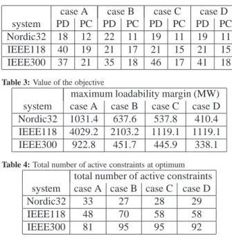
4.1 Maximization of Power System Loadability We now focus on the determination of maximum load-ability. We assume a homothetical load increase, i.e. all loads are increased proportionally with their base case consumptions, covered by the slack generator only. Computation of the maximum loadability is carried out for four different cases. The results relative of these cases are given in Tables 2, 3 and 4. Thus, Table 2 displays the number of iterations to convergence for both PD and PC algorithms, Table 3 provides the value of the objec-tive function (the maximal loadability margin), while Ta-ble 4 shows the number total of binding constraints at optimum.
Table 2: Number of iterations to convergence
case A case B case C case D
system PD PC PD PC PD PC PD PC
Nordic32 18 12 22 11 19 11 19 11
IEEE118 40 19 21 17 21 15 21 15
IEEE300 37 21 35 18 46 17 41 18
Table 3: Value of the objective
maximum loadability margin (MW) system case A case B case C case D Nordic32 1031.4 637.6 537.8 410.4 IEEE118 4029.2 2103.2 1119.1 1119.1
IEEE300 922.8 451.7 445.9 338.1
Table 4: Total number of active constraints at optimum
total number of active constraints system case A case B case C case D
Nordic32 33 27 28 29
IEEE118 48 70 58 58
IEEE300 81 95 95 92
Case A. The control variables are generators voltage, variables ratio of LTC transformers, shunts reactance and slack generator active output. The equality constraints are the bus active and reactive power flow equations (2) and (3). The inequality constraints include limits on trans-former variable ratio, shunt susceptance and generators voltage magnitudes only (4). The latter are allowed to vary between 0.95 and 1.05 pu.
The maximal loadability limit corresponds to an SNB, minimal voltages at that point being as low as 0.852 pu
(for Cigre32 system), 0.838 pu (for IEEE118 system) and 0.812 pu (for IEEE300 system). Obviously, most active constraints stem from generators voltage being at its max-imal limit because the higher the generator voltage, the larger the maximal loadability margin.
By way of comparison we also computed the basic load-ability margin. The latter was obtained without the help of available control means and by neglecting all opera-tional inequality constraints (4). The unknowns of the problem (1-3) are therefore the bus voltages (angle and magnitude) and the stress value only. Loadability mar-gins are 39% (for Cigre32 system), 16% (for IEEE118 system) and 8% (for IEEE300 system) less than the val-ues of Table 3 which emphasizes the positive impact of control means on loadability margin. In other words, the larger the number of control variables allowed, the higher the value of the maximal loadability margin. The load-ability limits obtained also correspond to an SNB. Case B. With respect to the case A we add reactive out-put limits for generators while keeping the same control variables. As expected, one obtains a smaller maximum loadability margin as in the case A because, for the same control variables allowed, the larger the number of con-straints the lower the maximal loadability margin. The maximal loadability point is again an SNB, while 5, 21 and 29 generators reach their maximum reactive capabil-ity for the Cigre32, IEEE118 and IEEE300 systems. Note that in all tests carried out we have not encountered an BP limit point.
Case C. We additionally include bounds on voltage mag-nitudes (0.95 and 1.05 pu) also for all buses other than generators while keeping the same set of controls. Obvi-ously, the maximal loadability margins are lower than in the previous case. Some voltages reaching their minimal bound prevent to obtain a higher margin.
Case D. We finally add current constraints for all branches while playing on the same control means. Ob-serve that for the IEEE118 system adding thermal con-straints does not influence the value of the maximal load-ability margin since no such constraint is active at opti-mum. Conversely, the margin decreases for the Cigre32 and IEEE300 systems where one and respectively two branches current constraints are active at optimum, and that together with few voltage magnitudes being at their minimal bound.
For comparison purposes, under the same assumptions as in the case C, we relax significantly bounds on voltage magnitudes at all buses which are now (0.90 and 1.10 pu) instead of (0.95 and 1.05 pu). Generally, the larger the bounds on voltage magnitudes, the higher the total num-ber of constraints active at optimum, as illustrated in Ta-ble 5. In this taTa-ble columns labeled with I (resp. II) cor-respond to the case C experiment (resp. the new case) columns V , Qg, r and b show the number of active constraints corresponding to voltages, reactive power of generators and shunt reactance respectively. Obviously, maximum loadability margins significantly increase with
85%, 106% and 30% for Cigre32, IEEE118 and IEEE300 systems, which shows that the objective is very sensitive to the choice of these bounds.
Table 5: Number and type of active constraints for different bounds on
voltage magnitudes system V Qg r b total I II I II I I I II I II Nordic32 17 14 5 5 0 0 6 7 28 26 IEEE118 27 25 21 31 0 1 10 13 58 70 IEEE300 57 62 29 30 4 3 5 5 95 100
As regards the IP algorithms performance to solve this highly nonlinear problem, the PC one is very robust in all cases, while the PD one converges very slowly in some cases (see Table 2). This behaviour is attributed to a poor centrality of iterations at some iterations [5].
Concerning the initial value of the barrier parameter, best results were obtained when µ0 ∈ [1, 100] for the PD al-gorithm and µ0∈[0.1, 10] for the PC one.
4.2 Minimization of Amount of Load Shedding We now concentrate on minimizing the amount of load shedding in an infeasible power system situation such that an equilibrium point is restored. We assume that load shedding is done under constant power factor at each bus but results will only be presented in terms of MW. Max-imum allowable fraction of load shedding is of10% at each load bus.
The test systems are driven to infeasible states as follows. For all the systems we first compute the loadability limit (corresponds to an SNB) by running the OPF with re-laxed reactive power limits of generators while freezing all control means. At this limit, one simulates a harmful contingency, for Cigre32 and IEEE118 systems, while in-creasing all loads with still 5% beyond the SNB for the IEEE300 system.
Four cases are analyzed in the sequel in order to evalu-ate the impact of various control variables on the objec-tive. Results relative to these experiments are provided Tables 6, 7 and 8. Thus, Table 6 presents the number of iterations to convergence of both algorithms under study, Table 7 displays the value of the objective, while Table 8 shows the number total of binding constraints at optimum (nac) as well as the number of load curtailed (nls).
Table 6: Number of iterations to convergence
case E case F case G case H
system PD PC PD PC PD PC PD PC
Nordic32 12 8 13 8 25 11 20 12
IEEE118 17 11 16 12 47 10 15 18
IEEE300 13 9 19 12 20 13 18
Table 7: Value of the objective
minimal load shedding(MW) system case E case F case G case H
Nordic32 501.7 352.5 349.3 151.4
IEEE118 107.3 105.7 0.0 0.0
IEEE300 1128.6 1125.0 1078.8 900.8
Table 8: Total number of binding constraints at optimum (nac) and
number of load curtailed (nls)
case E case F case G case H system nac nls nac nls nac nls nac nls
Nordic32 20 14 32 9 32 9 48 5
IEEE118 88 17 94 17 91 0 91 0
IEEE300 175 108 183 91 196 88 253 80 Case E. The control variables are loads consumptions and slack generator active output. The equality con-straints are the bus active and reactive power balance (6 and 7). The inequality constraints include limits on load curtailment fraction only (8). After curtailing some loads (e.g. 17 loads out of the total of 91 for the IEEE118 sys-tem, see Table 8) an equilibrium point is restored. The latter corresponds to an SNB for all systems, fact which holds true at least as long as constraints on reactive limits or generators, voltage magnitudes and branch current are neglected.
Case F. With respect to the previous case, we now more-over allow shunts reactance as control variable and take into account their relative constraints (included into 9). As expected, the higher the number of controls available, the lower the value of the objective (see Table 7). Never-theless, except of the Cigre32 system, the effect of shunts under the minimal amount of load shedded is marginal. Of course, this effect depends on the contingency applies as well as the shunt location. Obviously, the higher the number of controls available, the larger the number of load curtailed and the higher the number of active con-straints (see Table 8).
Case G. Comparatively with case F we also allow con-trollable ratio of transformers as control variable and add their relative constraints (9) to the optimization problem. This slightly decreases the value of objective for Cigre32 and IEEE300 systems. Conversely, the infeasibility is completely solved in the IEEE118 system and that with-out shedding load, a system equilibrium point close to the SNB being restored.
Case H. We finally add generators voltages as control variables and consider their respective constraints (9). Objectives are more (Cigre32 system) or less (IEEE300) improved while the number of loads curtailed decrease again.
As a general remark, the optimization algorithm tends to put the whole curtailment effort on the most efficient loads and, by consequence, at the optimum some loads are curtailed at maximum, others are not curtailed at all, while very few ones (generally one) are lying in between bounds.
Now we briefly present some results for the Cigre32 sys-tem only. So far we have requested only that load shed-ding to ensure an equilibrium point when the system is in an infeasible state. In order to obtain meaningful op-erating points and not just voltage stability limits one can add to the problem other operational constraints. Let thus consider the case H and to moreover request that all gen-erators have their reactive output between limits. Note
that at the solution of case D, 10 generators exceed their maximal reactive capability. To solve this case, 9 loads are curtailed of a total value of 305.8 MW, i.e. 154.4 MW more than for the case H (see Table 7). PD (resp. PC) algorithm converges in 17 (resp. 13) iterations while 4 generators attain their maximal reactive capability at op-timum. At this point, one branch is overloaded while three others are very close to their maximal admissible currents. Adding all branch constraints to the problem and running the OPF again yield an overall load shed-ding of 321.2 MW distributed over the same 9 loads. PD (resp. PC) algorithm converges in 25 (resp. 12) itera-tions while, at optimum, the same 4 generators maximal reactive power limit are active as well as a branch cur-rent. Note finally that both algorithms can successfully deal with more severe branch overload situations. PC algorithm performs very well also for this (very) non-linear problem. On the other hand, the PD fails to solve a case (case H for the IEEE300 system, see Table 6), while converging very slowly in the case G for the IEEE118 system.
As regards the initial value of the barrier parameter, best results were obtained when µ0∈[1, 10] for the PD algo-rithm and µ0∈[0.1, 1] for the PC one.
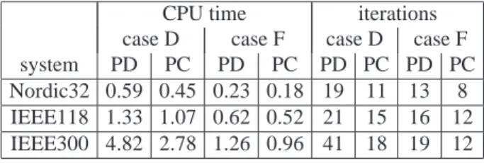
CPU time. Table 9 provides a sample of CPU time (in seconds) for both algorithms when studying cases D and F. The CPU time concerns the optimization process only except of processing data and display of results.
Table 9: Sample of CPU time and iterations number for PD and PC
algorithms
CPU time iterations
case D case F case D case F
system PD PC PD PC PD PC PD PC
Nordic32 0.59 0.45 0.23 0.18 19 11 13 8 IEEE118 1.33 1.07 0.62 0.52 21 15 16 12 IEEE300 4.82 2.78 1.26 0.96 41 18 19 12 Clearly, the PC algorithm outperforms the PD one in terms of both CPU time and iterations count.
5 CONCLUSION
This paper has presented two interior point method based OPF applications, namely the maximization of power system loadability and the minimization of the amount of load shedding, while comparing the performances of PD and PC algorithms on three test systems of reason-able size.
Our experience with these two algorithms confirms other results from the literature, that is, most of the time the PC algorithm outperforms the PD one in terms of CPU time (and thereby iterations count), both converging to the same optimum. Due to the high nonlinearity of the OPF problems studied some failures or very slow con-vergence of the PD algorithm have sometimes been ob-served. On the other hand, the PC algorithm proved very robust in all cases studied.
Both algorithms can rather easily handle problems when a significant number of active constraints is active at op-timum. Admittedly, the number of binding constraints at optimum may slightly increase the number of iterations to convergence, feature which is more pronounced for the PD algorithm. It is noteworthy that the number of itera-tions to convergence is little sensitive to the size of the system.
We finally mention that the versatileness of our OPF was also revealed when testing other two typical objectives, namely the minimization of the generation cost and the minimization of transmission active power losses [6]. For these problems both algorithms behave extremely well, the PC one slightly outperforming the PD one.
For the time being our approach of loadability limit com-putation and minimal load shedding can be carried out for a specified system topology at a time. A future extension of this approach concerns the handling of contingencies for both objectives, as in a security constrained OPF.
Acknowledgements
This work is funded by the “R´egion Wallonne” in the framework of the project PIGAL (french acronyme of Interior Point Genetic ALgorithm), convention RW 215187.
REFERENCES
[1] J. Carpentier “Contribution `a l’´etude du dispatch-ing economique”, Bulletin de la Societ´e Francaise d’Electricit´e, vol. 3, pp. 431-447, 1962
[2] R.D. Christie, B.F. Wollenberg, I. Wangensteen “Transmis-sion management in the deregulated environment”, Pro-ceedings of the IEEE, vol. 88, pp. 170-195, 2000
[3] A.V. Fiacco, G.P. McCormick “Nonlinear Programming: Sequential Unconstrained Minimization Techniques”, John Willey & Sons, 1968
[4] S. Mehrotra “On the implementation of a primal-dual inte-rior point method”, SIAM Journal on Optimization, vol. 2, pp. 575-601, 1992
[5] J. Gondzio, “Multiple centrality corrections in a primal-dual method for linear programming”, Computational Op-timization and Applications, vol. 6, pp. 137-156, 1996 [6] F. Capitanescu, M. Glavic, L. Wehenkel, “An interior-point
method based optimal power flow”, ACOMEN conference, Ghent, Belgium June 2005, 18 pages
[7] I. Dobson, “Observations on the Geometry of Saddle Node Bifurcation and Voltage Collapse in Electric Power Sys-tems”, IEEE Transactions on Circuits and Systems – I, vol. 39, pp. 240-243, 1992
[8] I. Dobson, L. Lu, “Voltage collapse precipitated by the im-mediate change in stability when generator reactive power limits are encountered”, IEEE Transactions on Circuits and Systems – I, Vol. 45, pp. 762-766, 1992
[9] T. Van Cutsem, C. D. Vournas, “Voltage Stability of Elec-tric Power Systems”, Kluwer Academic Publishers, 1998
[10] V. Ajjarapu, C. Christy, “The continuation power flow: a tool for steady state voltage stability analysis”, IEEE Transactions on Power Systems, Vol. 7, pp. 416-423, 1992 [11] S. Granville, J.C.O. Mello, A.C.G. Mello ”Application of interior point methods to power flow unsolvability”, IEEE Transactions on Power Systems, Vol. 11, pp. 1096-1103, 1996
[12] G. D. Irrisari, X. Wang, J. Tong, S. Mokhtari ”Maximum loadability of power systems using interior point nonlinear optimization methods”, IEEE Transactions on Power Sys-tems, Vol. 12, pp. 162-172, 1997
[13] C. Moors, T. Van Cutsem, “Determination of optimal load shedding against voltage instability”, PSCC Conference, Trondheim (Norway), pp. 993-1000, 1999
[14] T. Van Cutsem, C. Moisse, R. Mailhot,”Determination of secure operating limits with respect to voltage
col-lapse”,IEEE Transactions on Power Systems, Vol. 14, pp.327-335, 1999
[15] G.L. Torres, V.H. Quintana ”An Interior-Point Method for Nonlinear Optimal Power Flow Using Rectangular Coordi-nates”, IEEE Transactions on Power Systems, Vol. 13, No. 4, pp. 1211-1218, 1998
[16] W.D. Rosehart,C.A. Canizares, V.H. Quintana “Multiob-jective optimal power flows to evaluate voltage security costs in power networks”, IEEE Transactions on Power Systems, vol. 18, pp. 578-587, 2003
[17] C. Roman, W.D. Rosehart “Complementarity model for generator buses in OPF-based maximum loading prob-lems”, IEEE Transactions on Power Systems, vol. 20, pp. 514-516, 2005