HAL Id: hal-03219182
https://hal.archives-ouvertes.fr/hal-03219182
Preprint submitted on 6 May 2021HAL is a multi-disciplinary open access archive for the deposit and dissemination of sci-entific research documents, whether they are pub-lished or not. The documents may come from teaching and research institutions in France or abroad, or from public or private research centers.
L’archive ouverte pluridisciplinaire HAL, est destinée au dépôt et à la diffusion de documents scientifiques de niveau recherche, publiés ou non, émanant des établissements d’enseignement et de recherche français ou étrangers, des laboratoires publics ou privés.
Financial planning & optimal retirement timing for
physically intensive occupations
Edouard Ribes
To cite this version:
Edouard Ribes. Financial planning & optimal retirement timing for physically intensive occupations. 2021. �hal-03219182�
1
Financial planning & optimal retirement
timing for physically intensive occupations
24/04/2021
Edouard Ribes, CERNA Mines Paristech1 Abstract.
On average, O.E.C.D. statistics2 shows that 4 out of 10 workers in developed geographies occupy a “blue-collar” type of position. Since those professions are physically demanding and come with a toll on one’s health (which in turns translate into additional healthcare expenses), the length of an individual’s active period must be carefully weighted.
This paper therefore offers a financial model (and its subsequent program) to help make such decisions. It notably shows that whilst most developed countries require individuals to work for about 40 years, early retirement is a suitable option when healthcare prices are high.
This paper also shows that financial literacy has a significant impact on retirements behaviors. For those with a strong predilection for present consumption and little interest in savings and investments, retirement is not an option. In those cases, the financial pressure associated to the healthcare system translates into either an incentive for them to work until the end of their life or not to enter the labor market at all.
Keywords. Health; Retirement; Financial planning
Introduction
Research in the field of financial planning dates back as far as the 60s. Historically speaking, associated research has however been heavily geared towards company/firm level applications (e.g. optimal trading programs for banks, investments scheduling applications for industrial companies, workforce/manpower planning etc..) (see (Andriosopoulos, Doumpos, Pardalos, & Zopounidis, 2019) for a review and discussion).
This is something that is starting to change. The digitalization of the financial eco-system (i.e. the so called “fintech” movement) has been reducing financial intermediation costs and therefore has led to a democratization of financial services for retail investors (Gomber, Kauffman, Parker, & Weber, 2018). In the case of financial planning services, this means that services are no longer limited to firms but are being offered via platforms to individuals (independently of their wealth profile).
At this level, financial planning is about helping individuals achieve a balanced budget meeting their everyday needs. Those needs, according to the definition proposed by the O.E.C.D, include housing, food, clothing, leisure, and health. Among those elements, health has started to take in increasingly prominent place in developed countries. Associated expenditures have been on the rise, up from 3.8% of household budgets in the 60s to 8%+ in the late 90s (Nghiem & Connelly, 2017). Drivers causing this increase are well-known (income growth, the ageing of the population, technological progress, and the widespread availability of health insurance). But if the situation has started to stabilize in certain countries such as the E.U. ones (Hitiris & Nixon, 2001), the situation is
1
Contact: [email protected]
2 not yet under control everywhere across the globe. One of the worst scenario (for developed countries) is for instance encountered in the US where about 25% of the population cannot, as of today, cope with health related bills (Dickman, Himmelstein, & Woolhandler, 2017) and where the situation keeps on worsening (according to the O.E.C.D statistics health expenses in the US represented 20%+ of households expenditures in 2018).
One of the acknowledged problems associated with raising healthcare costs has been that inequalities across households have been increasing. This is for instance reflected by the fact that nowadays life expectancy between the wealthiest constituents of the population and its lower quartile (income wise) varies by 10+ years (Chetty, et al., 2016). It is also made blatant by the fact that an important fringe of the population (8%+ in the US (Berchick, Hood, & Barnett, 2019), 2%+ in the EU (Toth, 2019)) still cannot afford/ does not have access to basic medical insurance. Additionally, primary health insurance scheme coverage can vary widely. As a result, the least wealthy part of O.E.C.D countries’ population has a hard time managing their budget and health bills. Health expenses are however pervasive in the sense that they increase exponentially over time as one’s abilities start to naturally decline (Shang & Goldman, 2008). This is normally met by constituting precautionary savings whilst active (Cagetti, 2003). For the lower quartile (income wise) of O.E.C.D. populations, a first challenge lies with individual’s saving behavior (i.e. less wealthy individuals tend to live in the now – a well know behavioral anomaly (Love & Phelan, 2015)). An additional challenge arises for those involved in physically demanding occupations which are having an impact on their health. In this case, a potential conflict arises between (option A) working and saving whilst deprecating their health stock at a faster pace than what would naturally occur and (option B) stop working but having to face important healthcare related bills3. In short, when does it become optimal to retire? The perspective taken in this article is that the difficulty faced by those parts of the population could be mitigated by providing them with cheap (and potentially free) financial planning tools to inform their decisions, which is where the “fintech” movement could play a part.
This article will therefore describe the mechanics of a health economic model which could easily be implemented into a SaaS platform to address this need (i.e. provide individuals in physically demanding occupations with an optimal financial blueprint). In terms of structure, this paper will start by a literature review of the health economics models currently in place and use it to highlight the theoretical contribution of the article (section I). Section II to IV will then gradually build the model and exemplify its properties. Section V will finally offer a discussion around the impact of location/market specific parameters as well as individuals’ time preference on the proposed financial plan. A short conclusion will then follow.
3
Note that in this context, health issues refer to conditions that cannot be recovered from (e.g. chronic musculoskeletal conditions), but only controlled by “artificial” means (i.e. a therapy).
3
I – The current theoretical health economics context:
Modeling in the health economics space is rooted in the concepts developed by (Grossman, 1972). In this framework, an individual possesses a stock of health, which naturally deprecates over time. Individuals can then invest in their health stock (through healthcare expenditures for instance) to maximize their own utility over their entire lifecycle. This seminal model was then further generalized by (Muurinen & Le Grand, 1985) to notably study the impact of education on individual’s health-related investments decisions.
Grossman’s model has sparked several discussions over the past decades as the academic community has been challenging some of its underlying assumptions. A first wave of comments made by the community aimed at improving the way the model accounts for the human aging process. This included challenges around the underlying assumption around an individual’s ability to repair/replenish one’s health stock (Case & Deaton, 2005) (Galama T. , 2015) or its decontextualized view of an individual’s life (family, social status etc… ) (Kohn & Patrick, 2008) (Sepehri, 2015). Additional comments also emerged around the model’s complexity and its lack of tractability (i.e. the absence of closed forms solutions) (Strulik, 2015).
Despite some critics, the seminal nature of the concepts behind Grossman’s model is well recognized and it gave birth to a large empirical literature (see (L’haridon, Messe, & Wolff, 2018) for a review). The best route to further our knowledge from a theoretical standpoint was then highlighted in the final address of (Muurinen & Le Grand, 1985) and remains unchanged as of today. Their recommendation was not to try to challenge Grossman’s framework but rather to build simpler sub models out of it and use them to study very specific questions.
One of those modeling questions (which has recently gained traction amongst the academic community) pertains to the mechanisms linking health and an individual’s retirement decisions. One of the reasons for this interest lies in the fact that if within developed countries governments have started to increase the legal retirement age4 , an increasingly significant part of the population (25%+) is still retiring early (Beehr, 1986). Modeling efforts exploring the motivations for this unexpected individual behavior fall in two main categories.
On one hand, models have been used to assess the effect of individual income on health (including expenditures) and retirement age. (Dalgaard & Strulik, 2012) found that an increase in individual income was leading to higher health and that utility considerations would in turn lead individuals to seek an early retirement. This was also echoed in (Bloom & Canning, 2014) and (Kuhn, Wrzaczek, Prskawetz, & Feichtinger, 2015) but somewhat challenged in (Prettner & Canning, 2014), whose proposition was that early retirement was mainly driven by monetary incentives and institutional constraints rather than by income considerations. Another interesting view on the topic is the one of (Galama, Kapteyn, & Fonseca, 2013) whose model shows that workers with higher human capital / education invest more in health and, because they stay healthier, retire later than those with lower human capital whose health deteriorates faster.
On the other hand, specific models have also been used to assess the effects of specific biological facts on retirement decisions. For instance, (Lau, 2012) studied the effects of changing mortality
4
Notably to account for the recent increase in life expectancy and the subsequent financial burden associated to public pension.
4 rates across individuals’ lifecycle5 and has shown that mortality reductions at older ages delay retirement unambiguously, but that mortality reductions at younger ages may lead to earlier retirement. More recently, other models (such as the one of (L’haridon, Messe, & Wolff, 2018)) have also started to explore the problem through another angle - how does activity reduction (because of retirement) benefit health.
The idea of this paper is to revisit the question of the optimal retirement age by blending biological and income considerations. The proposal is to review how the retirement decision is made in the case of individuals whose occupation naturally takes a toll on their health. This applies for instance to all “blue collar” workers who still represent as of today an important share of the active population of developed countries (for instance about 40% in the UK and in Germany according to the O.E.C.D WISE database). From what can be seen on the health economics literature, the problem appears unaddressed. Besides, it increments the work done by (Galama, Kapteyn, & Fonseca, 2013) by looking at low-income occupations and studying what happens when health is not a product of an investment but the motor for income generation. Additionally, it appears to address some of the recommended areas of future investigations (notably around contextualized retirement decisions) suggested by (Sepehri, 2015).
II – A simple retirement model:
There are two periods in an individual’s life. During the first period, the person is a productive member of the society and earns a net income every year. This represents a person’s contribution as a worker. During the second period, the canonical view (Skirbekk, 2004) is that a person’s abilities decline to the point that no income can be generated through labor. Two income sources are then available. On one hand, the state provides a public pension to replace one’s income at a rate6 (annuities scheme)7. On the other, individuals can withdraw some of the accumulated capital ( ) during their productive phase. This capital stems from saving a portion of its income during the activity period and investing it in financial products (with an expected return of ).
The lifecycle of an individual can then be described by two main parameters: the length of its active/ productive period ( ) and the length of its retirement phase ( ). Being active generates a total of and savings realized during that time yield a capital of
= . .1+ +1 1 . During the retirement phase, the individual gets a yearly annuity of . . The annuity is completed by withdrawal(s) , whilst the acquired capital still yields dividends (i.e. ). If the individual has no time preference, the earnings associated to his/her lifecycle can be summarized as:
Given that an individual cannot withdraw more than the accumulated capital, the following set of recursive constraints appears:
5
Rapid science advances have led to a drastic reduction of mortality rates for active individuals and have improved our control over major health issues. The pace of the change is such that individuals can benefit from those progresses during their lifetime.
6
As a result, when retiring, an individual gets a pension worth until death
7
Note that it is not the aim of this paper to discuss potential public pension policies adjustments. As such, both replacement rates (and taxes) are assumed constant over time. This could however represent an area of additional research.
5
In this context, assume that both life cycle periods and individual income are given exogenously (i.e. ). The underlying idea behind this assumption would be that one’s productive abilities (incl. wages) are not something he/she can choose (i.e. and ), nor is his/her life expectancy (i.e. ). If this is something that will be re-discussed later, this means, for now, that an individual’s earning is potentially subject to an optimization in terms of a saving and withdrawal program. This then translates into the following constrained linear programming maximization problem:
Property 1. In the absence of time preference, an individual would seek to maximize his/her total
earnings over his/her lifecycle (i.e. ) by investing all of his/her income during the activity period (i.e.
) and by only withdrawing money at the very last period of his/her life (i.e. . Total earnings are then given by:
Proof. If an individual as 1€ available in time , he/she can consume it immediately or invest it and consume it after periods yielding an output of . In the absence of time preference or constraints, individuals will therefore save to maximize their wealth. The same behavior will conduct them to delay withdraw as much as possible.
The behavior described by property (1) revolves around accumulating wealth. Without any constraint on his/her budget, a wealth maximizing individual will simply invest and stock capital to finally pass it to the next generation. Note that this will be further discussed in the following sections, as individuals notably need to protect a portion of their income to ensure basic life expenditures (e.g. food, health etc…).
The behavior described by property (1) revolves around accumulating wealth. Without any constraint on budget, a wealth maximizing individual will simply invest and stock capital to finally pass it to the next generation. Note that this will be further discussed in the following sections, as individuals notably need to protect a portion of their income to ensure basic life expenditures (e.g. food, health etc…).
Example. Assume that an individual is active for about years with an income of and lives another years when retired. Assume that the individual lives in a market where he/she can invest in a financial product yielding a return per year. Under the modeling assumptions described in this section, individuals will invest all their earnings while active, get their pensions and only make a withdrawal before dying. The total wealth ( ) collected over their lifecycle is then linearly increasing with the replacement rate of the pension they get. It ranges from when the replacement rate is worth to for replacement rate at .
6 This behavior is optimal whatever the structure of the lifecycle (i.e. whatever the length of the active (resp. retirement) period [ (resp. )]). Now, while individuals have little control over their life expectancy (i.e. ), they can potentially choose whether to stay active or to retire. In other more quantitative terms, an individual can, given the results highlighted in property 1, solve the following additional optimization program:
Lemma 1. In the absence of time preferences or budget constraints over their lifecycle and assuming
the rate of return of financial products are small (i.e. ), individuals choose to retire as late as possible to maximize their wealth.
Proof. The result displayed in lemma 1 can be obtained by leveraging the result highlighted in property (1) and solving . In this case, the optimal length of the activity period is given as
. Given that
and > if . ).
III – Accounting for living standards:
The previous section has shown that individuals seeking to maximize their wealth save and capitalize as much as possible when they are not subject to any constraints (property 1). In that set up, they also tend to retire as late as possible (lemma 1). To make the model more realistic, livings standard must yet be accounted for: individuals indeed need to earn at least to cater for their primary needs8 (food/housing etc…). This adds a series of additional constraints to the problem described in the previous section:
When accounting for living standards, three potential cases appear. First, an individual can face difficulties providing for his/her primary needs while active (i.e. ). In this instance, the problem will also carry on during the retirement period as public pension only provide an annuity equals to a fraction of the wages earned while working (i.e. ) and no savings are available. The discussion of this case is not in scope for this study.
The second possibility would be that an individual earns enough while active and that the public pension enables him/her to live comfortably (i.e. ). In this case, the problem is similar to the one described in the previous section: the individual will accumulate capital up to and retire as late as possible if given the choice. Eventually the individual could even continue saving while retired as his/her needs are met.
But in a number of occasions, if individuals earn enough while active, public pensions are not sufficient to enable them to live up to their own standards (i.e. ).
8
For now (i.e. throughout section III), livings standards will be assumed constant. This will however be subject to a revision in the next section.
7
Lemma 2. When public pensions are not sufficient to ensure a living standard of , for an individual
to be able to withdraw just enough to meet his/her standards (i.e. ), the length of his/her activity period must be such that:
Corollary 1. Retired Individuals withdrawing to meet their livings standards will see
their capital decrease unless the following condition is met:
Proof. When an individual withdraws , his/her capital follows This translates into:
Since , the condition highlighted in corollary 1 simply ensures that an individuals’ capital is always positive and grows. Finally, meeting the condition (with ) yields the result highlighted in lemma 2.
Property 2. When public pensions are not sufficient to ensure a living standard of , individuals who
maximize their wealth ( ) and who have worked long enough (see lemma 2) save as much as possible while active (i.e. ) and then withdraw the minimum necessary to reach their standard (i.e.
). Their overall wealth is then given by:
Proof. Property 2 naturally stems from the considerations developed in property 1.
Lemma 3. Individuals who seek to maximize their wealth work for as long they can.
Proof. When individuals do not have enough savings to ensure a proper living standard during retirement, they keep on working. Those with sufficient savings have a wealth (see property 2) such that:
Example. Consider the example developed in the previous section9 (i.e. ). Lemma 2 can be used to understand how long individual need to work (i.e. ) to have enough capital to sustain a given living standard (i.e. ) until their death (i.e.
9
Note that in this context, the early stage of an individual’s life (i.e. the first 20 years) are excluded of the analysis. This period is normally dedicated to education and does not enable individuals to be productive members of the society.
8 where does the capital availability boundary stand?). Conversely, corollary 1 can be used to assess how long does an individual need to work to keep capitalizing whilst retired (i.e. where does the capital increase boundary stands?). Results presented in figure 1 show that for an individual to cover living standard expenses of , he/she must at least work for a period of 30 years. Besides, he/she will only generate some excess of capital while retired if they have worked long enough for the capital to be sufficient to generate meaningful dividends (i.e. years).
Figure 1 - Duration of the activity period to achieve certain capital related objectives under living standards constraints. In summary, this section has shown that the financial plan of a person who must meet a set living standard is not so different from the one of unconstrained individuals. Over their lifecycle, constrained persons will indeed seek to work for as long as possible. The only difference revolves around whether they will consume or keep on increasing their capital, which has been shown to be dependent on the length of the activity period.
IV – Impact of health on retirement decisions:
Recent research has shown that the amount required to ensure a decent living (i.e. ) is actually variable during an individual lifecycle. A key component driving individual expenditures is indeed related to out-of-pocket expenses as individuals age and their health deteriorates (i.e. ). This decline is due to two main factors. On one hand the natural ageing process comes with increasing health shocks. On the other, labor further erodes one’s health capital10. Therefore, when planning for their financial well-being, individuals are potentially faced with a challenge: if being active increases their wealth as they can invest a portion of their income and yield dividends, it may also lead to future financial hurdles. This section will thus build upon the previous ones by embedding notions of variable health expenditures in the proposed lifecycle model. The resulting model will then be analyzed to understand how individuals can optimally plan their finances and organize their lifecycle.
Over each period of time (e.g. a year), individuals face some health challenges which are taking them a portion of their available time (s.t. ). Every moment spent in this
9 state comes at a cost11 . Assuming that their overall living expenditures are mainly evolving according to his health status, their living standard can be modeled as: .
To understand how health considerations can impact an individual’s decisions, additional modeling is required. Assume that the portion of time where an individual is healthy decrease at a rate over each period (i.e. ) and that the beginning of one’s life is exempt of health issues (i.e. ). Now, a simple way of looking at the rate at which health declines is to assume that an inactive individual experiences a natural deterioration at a rate , whilst working comes with some extra burden and a rate of health decay worth
. In this context (and leveraging the notations introduced in the previous sections), health issues obey the following rules:
Lemma 4. When faced with variable health expenditures, an individual who saves and invests as
much as he/she can while active (with an expected rate of return of ) therefore accumulates a capital worth:
Proof. At every time step active individuals can save up to . The capital they accumulate over active periods is therefore given by: . Leveraging equation (1) then yields the proposed result.
Corollary 2. If individuals earn enough while active to cover for the expenditures they would face in
the worst possible health conditions (i.e. ), the capital they accumulate while active keeps on increasing (i.e ). Otherwise (i.e. ), it is not interesting for an individual to work for more the following numbers of periods:
Lemma 5. Once retired, individuals, who withdraw the bare minimum necessary to meet their living expenditures (i.e. ), see their capital follow ( ):
Proof. Post retirement (i.e. ), individual’s capital evolution is driven by: . Leveraging equation (1) then leads to ( ):
11 In the paper, health issues are not assumed to impact individuals’ income during their working period (i.e.
remains unchanged). The idea here is twofold. First, health issues are relatively rare whilst working, because deferred to a later part of life. Second, public health insurances provide coverage for the couple of days where individuals are on sick leave. A natural extension (although not in scope of this paper) could be to consider the impact of an additional private health insurance on the retirement decision.
10
Further developments then yield the proposed result.
Note that lemma (5) implies that individuals whose pension is high enough to cover the worse possible health expenditures (i.e. ) always experience an increase in capital.
Property 3. In a context where health deteriorates over a lifecycle of length , individuals (active over
periods) maximize their wealth by investing as much as possible while working and then only withdrawing the bare minimum during their retirement. Their resulting wealth is given by:
Equation (4) can then be used to assess the length of an individual’s activity period which maximizes their wealth. If this problem does not lead to a closed formula, it can easily be solved through simulations (see the following example).
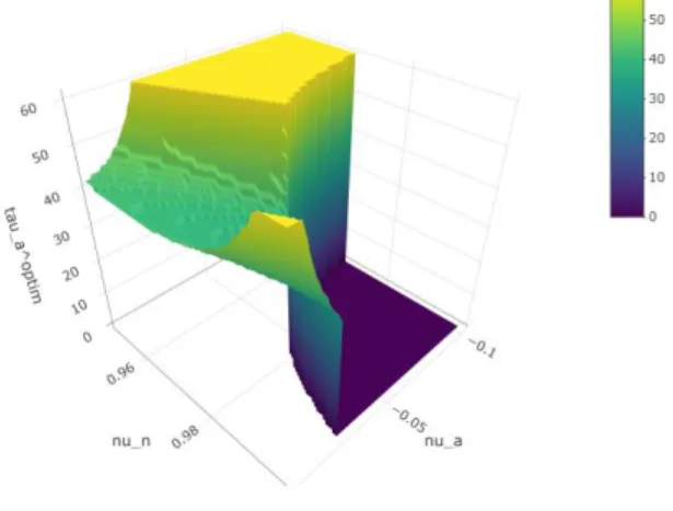
Example. Assume that an individual lives in a socio-economic context similar to the one depicted in the previous sections12 (i.e. ) and that health care expenses can rise up to . A simple grid search can then be used to assess what is the optimal activity period for a given health decay profile . Results (display in figure 2) show that 3 scenarios can arise. When the natural decay rate of individuals’ health is low (i.e. , they will not work at all if labor decreases their health in an important manner (i.e. in the example). A second possibility consists in having individuals work until the end of their life. This occurs when health conditions are poor (i.e. ) or excellent (i.e. & . An intermediary case then arises where workers optimize their activity period. Note that the higher the healthcare expenses, the more workers are interested in optimizing the duration of their activity period (see figures 3 & 4).
12
The underlying assumption here is that everyone has access to financial products. Given that equity investments are nowadays fully democratized by online brokerage platforms (e.g. Degiro, Robinhood etc…), access is a question of financial literacy. Some aspects of this problem will be further discussed in section V.
11 Figure 2 - Optimum activity period length (I=
Figure 3 - Optimum activity period length (I=
Figure 4- Optimum activity period length (I=
12
V – Discussion:
a. Sensitivity of individual’s retirement behavior on the local context:
Given an occupation (and the associated health stock impact), the retirement timing selected by an individual can vary based on two exogeneous (and location based) components. On one hand, retirement will be impacted by the local price of healthcare, reflected by the ratio . On the other, the retirement decision will change depending in the level of replacement rate (i.e. ) offered by local public pension schemes. For instance, average replacement rates in the U.K. are around 10% versus 60% to 80% in southern European countries such as France, Italy or Spain.
A sensitivity analysis was therefore performed with the proposed model to understand the impact of location/ social context (i.e. a pair of parameters ) on individuals’ behavior. Results displayed on figure 5 show that the retirement decision is more sensitive to the price of healthcare than to the replacement rates offered by public pensions. As expected, the more expensive the healthcare system compared to their job-dependent income, the longer individuals are incentivized to work. Besides, the sensitivity analysis also shows that if public pensions are too high and if there is no eligibility criteria for public pensions (in terms of numbers of years/ months spent being active), individuals have no incentive to work.
Figure 5 -Optimum activity period length ( , )
A natural sub-area of discussion then arises as most states/countries offer public pensions which size depends on the amount of time spent contributing to the society (i.e. ). Looking at the rules framing public pensions schemes across developed countries, a few commonalities appear. Usually, replacement rates evolve between a maximum and a minimum and if the
maximum replacement rate can be claimed after a period of activity, early retirement leads to a loss of points per year.
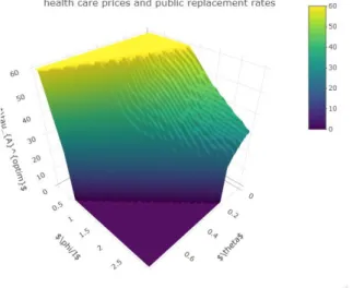
Such a functional form can easily be embedded equation (4) to assess how optimal retirement timing evolves depending on healthcare prices. Assuming for instance that =60%, ,
and , the proposed model can then be used to decide when to optimally retire depending on healthcare prices. Results displayed in figure 6 show that as long as maximum healthcare prices are below annual working wages (i.e. ), individuals will keep on working until they die and that individuals do not work if healthcare prices are five times higher than working
13 wages (i.e. deprecating one health stock is too expensive). Interestingly, when , individuals retire early. This could explain why individuals in physically demanding and low-income occupations could be driven towards early (if not very early) retirement.
Figure 6 - Optimum activity period length based on healthcare prices ( , )
b. Sensitivity of the proposed financial plan to individual’s time preferences:
Looking back at the insights derived from the literature, it also appears that individuals with physically demanding jobs not only have a low income but also present a lack of financial knowledge/ literacy (Love & Phelan, 2015). As a result, their time preferences are often biased towards the present and the decisions they make depart from canonical frameworks (from which the model developed in this paper is derived). An option to assess how such a behavior may impact the optimal financial and retirement plan proposed in the previous section consists in introducing a utility in the equation describing individual’s wealth ( ). Note that, in this context, represents the perceived utility an individual has of wealth in units of time. The outcome of this adjustment is that wealth decisions become a recursive program depending in the current point in time:
Two cases can then potentially occur. In the first instance, if an individual perceives that saving yields a better outcome than immediate consumption (i.e. , the plan highlighted throughout sections II to IV in terms of investments and withdrawal still holds. Consequently, individuals can also make an “early” retirement decision based on the physical hardship entailed by their occupation.
However, if individuals’ preferences are skewed towards the present (i.e. , they will postpone their investments. Given the recurring nature of those decisions, this means that, at every point in time, they will keep delaying the start of potential provisions (i.e. ) and won’t have any capital to withdraw from (i.e. ). Their overall wealth will therefore follow:
14
This type of behavior will also potentially impact the definition of an optimal retirement timing. When reviewing their options at a point in time individuals will indeed delay their retirement decision by one period as long as it appears in their interest to do so (i.e. ). This means that they will delay retirement if:
Now to progress further and qualify a potential delay in the retirement decision, it is necessary to assume a functional form for individual’s utility. Let us take two examples. In the first instance (scenario A), assume that individuals have hyperbolic time preferences (i.e. ). In this scenario, they will only invest if . Otherwise (i.e. when ), they will not have any capital available and when considering retirement, they will keep working if the following condition is met:
Similarly, let us consider a second scenario (scenario B) where individuals discount future preferences exponentially (i.e. assume .In this case, they will delay their investments if and when that is the case also delay their retirement if the next condition is satisfied:
Example. The functional forms highlighted in this sub-section can be used to compare the decision made by individuals on retirement timing based on their time preferences. Assume that individuals’ health stock is naturally decreasing at a rate , that their occupation yields a heath deprecation rate of . Also assume that replacement rates offered by the public pensions are worth and that financial investments yield a return of .
When individuals have hyperbolic time preference (scenario A), it can be seen from simulations that individuals either choose to work until the end of their life if healthcare expenditures are small compared their income or avoid work. Besides the more individuals prefer the present (i.e. the higher ), the higher their tolerance towards an expensive healthcare system (see figure 7). The same pattern holds for individual with exponential time preferences (scenario B) (see figure 8).
15 Figure 7 - Sensitivity of retirement decisions to time preferences and healthcare prices (scenario A)
Figure 8 - Sensitivity of retirement decisions to time preferences and healthcare prices (scenario B)
Conclusion
Developed countries have an important share of workers who have physically demanding occupations. Since their activity exerts a toll on their health stock and since this deprecation comes at a price, they face a natural financial optimization problem in terms of the length of their activity period.
This paper thus offers a model to help them better assess the trade-offs between having relatively high earnings while active with an impact on their health and retiring. This naturally translates into a saving program and a recommendation around their optimal retirement timing. This article notably highlights that the more expensive the healthcare system, the earlier individuals should retire. For instance, under assumptions mimicking the public pension policies present in several developed countries, simulations shows that when healthcare expenses represent more than twice the annual earnings of a working person, individuals should retire 10 years earlier than what is recommended by most public mandated pension scheme.
Finally, this paper also illustrates that individuals’ behavior is yet subject change to change based on the time preferences of individuals. If they have a strong preference for immediate consumption, the model states that they will either work across their entire life or have no incentive to work at all. Behaviors in these cases are set by a combination of healthcare prices and time preferences.
17
Bibliographie
Andriosopoulos, D., Doumpos, M., Pardalos, P., & Zopounidis, C. (2019). Computational approaches and data analytics in financial services: A literature review. . Journal of the Operational
Research Society, 1581-1599.
Beehr, T. (1986). The process of retirement: A review and recommendations for future investigation. . Personnel psychology, 31-55.
Berchick, E., Hood, E., & Barnett, J. (2019). Health insurance coverage in the United States: 2018 .
Washington, DC: US Department of Commerce, 2.
Bloom, D., & Canning, D. M. (2014). Optimal retirement with increasing longevity. . The Scandinavian
journal of economics, 838-858.
Cagetti, M. (2003). Wealth accumulation over the life cycle and precautionary savings. . Journal of
Business & Economic Statistics, 339-353.
Case, A., & Deaton, A. (2005). Broken down by work and sex: How our health declines. In Analyses in
the Economics of Aging, 185-212.
Chetty, R., Stepner, M., Abraham, S., Lin, S., Scuderi, B., Turner, N., . . . Cutler, D. (2016). The association between income and life expectancy in the United States, 2001-2014. Jama, 1750-1766.
Dalgaard, C., & Strulik, H. (2012). The Genesis of the Golden Age-Accounting for the Rise in Health and Leisure. Univ. of Copenhagen Dept. of Economics Discussion Paper.
Dickman, S., Himmelstein, D., & Woolhandler, S. (2017). Inequality and the health-care system in the USA. The Lancet, 1431-1441.
Galama, T. (2015). A contribution to health-capital theory. . CESR-Schaeffer Working Paper. Galama, T., Kapteyn, A., & Fonseca, R. M. (2013). A health production model with endogenous
retirement. . Health economics, 883-902.
Gomber, P., Kauffman, R., Parker, C., & Weber, B. (2018). On the fintech revolution: Interpreting the forces of innovation, disruption, and transformation in financial services. . Journal of
Management Information Systems, 220-265.
Grossman, M. (1972). On the concept of health capital and the demand for health. Journal of Political
Economy, 223–55.
Hitiris, T., & Nixon, J. (2001). Convergence of health care expenditure in the EU countries. . Applied
Economics Letters, 223-228.
Kohn, J., & Patrick, R. (2008). Health and wealth: a dynamic demand for medical care. HEA 2007 6th
World Congress: .
Kuhn, M., Wrzaczek, S., Prskawetz, A., & Feichtinger, G. (2015). Optimal choice of health and retirement in a life-cycle model. . Journal of Economic Theory, 186-212.
L’haridon, O., Messe, P., & Wolff, F. (2018). Quels effets de la retraite sur la santé? Revue française
18 Lau, S. S.-R. (2012). Mortality transition and differential incentives for early retirement. . Journal of
Economic Theory, 261-283.
Lazear, E. (1979). Why is there mandatory retirement? Journal of political economy, 1261-1284. Love, D., & Phelan, G. (2015). Hyperbolic discounting and life-cycle portfolio choice. Journal of
Pension Economics and Finance.
Muurinen, J., & Le Grand, J. (1985). The economic analysis of inequalities in health. . Social science &
medicine, 1029-1035.
Nghiem, S., & Connelly, L. (2017). Convergence and determinants of health expenditures in OECD countries. . Health economics review.
Prettner, K., & Canning, D. (2014). Increasing life expectancy and optimal retirement in general equilibrium. Economic Theory, 191-217.
Rocha, R., Vittas, D., & Rudolph, H. (2010). The payout phase of pension systems: a comparison of five countries. . World Bank Policy Research Working Paper.
Sepehri, A. (2015). A critique of Grossman’s canonical model of health capital. . International Journal
of Health Services, 762-778.
Shang, B., & Goldman, D. (2008). Does age or life expectancy better predict health care expenditures? Health Economics, 487-501.
Skirbekk, V. (2004). Age and individual productivity: A literature survey. . Vienna yearbook of
population research, 133-153.
Strulik, H. (2015). A closed-form solution for the health capital model. . Journal of Demographic
Economics, 301-316.
Toth, F. (2019). Prevalence and generosity of health insurance coverage: a comparison of EU member states. Journal of Comparative Policy Analysis: Research and Practice, 518-534.