HAL Id: tel-00770844
https://tel.archives-ouvertes.fr/tel-00770844
Submitted on 7 Jan 2013HAL is a multi-disciplinary open access archive for the deposit and dissemination of sci-entific research documents, whether they are pub-lished or not. The documents may come from teaching and research institutions in France or abroad, or from public or private research centers.
L’archive ouverte pluridisciplinaire HAL, est destinée au dépôt et à la diffusion de documents scientifiques de niveau recherche, publiés ou non, émanant des établissements d’enseignement et de recherche français ou étrangers, des laboratoires publics ou privés.
AMELIORATION DE LA PRECISION ET
COMPENSATION DES INCERTITUDES DES
METAMODELES POUR L’APPROXIMATION DE
SIMULATEURS NUMERIQUES
Victor Picheny
To cite this version:
Victor Picheny. AMELIORATION DE LA PRECISION ET COMPENSATION DES INCERTI-TUDES DES METAMODELES POUR L’APPROXIMATION DE SIMULATEURS NUMERIQUES. Mathématiques générales [math.GM]. Ecole Nationale Supérieure des Mines de Saint-Etienne, 2009. Français. �tel-00770844�
N° d’ordre : 537MA
THÈSE
présentée par
Victor PICHENY
pour obtenir le grade de
Docteur de l’École Nationale Supérieure des Mines de Saint-Étienne
Spécialité : Mathématiques Appliquées
IMPROVING ACCURACY AND COMPENSATING FOR
UNCERTAINTY IN SURROGATE MODELING
soutenue à Gainesville (USA), le 15 décembre 2009
Membres du jury
Président : Bertrand IOOSS Ingénieur-chercheur, Centre à l'Energie Atomique, Cadarache
Rapporteurs : Tony SCHMITZ Bertrand IOOSS
Associate Professor, University of Florida, Gainesville, FL
Examinateur(s) : Grigori PANASENKO Nam-Ho KIM
Jorg PETERS
Olivier ROUSTANT
Professeur, Université Jean Monnet, St Etienne
Associate Professor, University of Florida, Gainesville, FL Professor, University of Florida, Gainesville, FL
Maitre-assistant, Ecole des Mines de St Etienne, St Etienne
Directeurs de thèse :
Raphael HAFTKA Alain VAUTRIN
Professor, University of Florida, Gainesville, FL Professeur, Ecole des Mines de St Etienne, St Etienne
Spécialités doctorales : Responsables :
SCIENCES ET GENIE DES MATERIAUX MECANIQUE ET INGENIERIE
GENIE DES PROCEDES SCIENCES DE LA TERRE
SCIENCES ET GENIE DE L’ENVIRONNEMENT MATHEMATIQUES APPLIQUEES
INFORMATIQUE IMAGE, VISION, SIGNAL GENIE INDUSTRIEL MICROELECTRONIQUE
J. DRIVER Directeur de recherche – Centre SMS A. VAUTRIN Professeur – Centre SMS
G. THOMAS Professeur – Centre SPIN B. GUY Maître de recherche – Centre SPIN J. BOURGOIS Professeur – Centre SITE E. TOUBOUL Ingénieur – Centre G2I O. BOISSIER Professeur – Centre G2I JC. PINOLI Professeur – Centre CIS P. BURLAT Professeur – Centre G2I Ph. COLLOT Professeur – Centre CMP
Enseignants-chercheurs et chercheurs autorisés à diriger des thèses de doctorat (titulaires d’un doctorat d’État ou d’une HDR)
AVRIL BATTON-HUBERT BENABEN BERNACHE-ASSOLANT BIGOT BILAL BOISSIER BOUCHER BOUDAREL BOURGOIS BRODHAG BURLAT COLLOT COURNIL DAUZERE-PERES DARRIEULAT DECHOMETS DESRAYAUD DELAFOSSE DOLGUI DRAPIER DRIVER FEILLET FOREST FORMISYN FORTUNIER FRACZKIEWICZ GARCIA GIRARDOT GOEURIOT GOEURIOT GRAILLOT GROSSEAU GRUY GUILHOT GUY GUYONNET HERRI INAL KLÖCKER LAFOREST LERICHE LI LONDICHE MOLIMARD MONTHEILLET PERIER-CAMBY PIJOLAT PIJOLAT PINOLI STOLARZ SZAFNICKI THOMAS VALDIVIESO VAUTRIN VIRICELLE WOLSKI XIE Stéphane Mireille Patrick Didier Jean-Pierre Essaïd Olivier Xavier Marie-Reine Jacques Christian Patrick Philippe Michel Stéphane Michel Roland Christophe David Alexandre Sylvain Julian Dominique Bernard Pascal Roland Anna Daniel Jean-Jacques Dominique Patrice Didier Philippe Frédéric Bernard Bernard René Jean-Michel Karim Helmut Valérie Rodolphe Jean-Michel Henry Jérôme Frank Laurent Christophe Michèle Jean-Charles Jacques Konrad Gérard François Alain Jean-Paul Krzysztof Xiaolan MA MA PR 2 PR 0 MR DR PR 2 MA MA PR 0 DR PR 2 PR 1 PR 0 PR 1 IGM PR 1 MA PR 1 PR 1 PR 2 DR PR 2 PR 1 PR 1 PR 1 DR CR MR MR MR DR MR MR DR MR DR PR 2 MR MR CR CR EC (CCI MP) MR MA DR 1 CNRS PR1 PR 1 PR 1 PR 1 CR CR PR 0 MA PR 0 MR MR PR 1
Mécanique & Ingénierie
Sciences & Génie de l'Environnement Sciences & Génie des Matériaux Génie des Procédés
Génie des Procédés Sciences de la Terre Informatique Génie Industriel Génie Industriel
Sciences & Génie de l'Environnement Sciences & Génie de l'Environnement Génie industriel
Microélectronique Génie des Procédés Génie industriel
Sciences & Génie des Matériaux Sciences & Génie de l'Environnement Mécanique & Ingénierie
Sciences & Génie des Matériaux Génie Industriel
Mécanique & Ingénierie Sciences & Génie des Matériaux Génie Industriel
Sciences & Génie des Matériaux Sciences & Génie de l'Environnement Sciences & Génie des Matériaux Sciences & Génie des Matériaux Génie des Procédés
Informatique
Sciences & Génie des Matériaux Sciences & Génie des Matériaux Sciences & Génie de l'Environnement Génie des Procédés
Génie des Procédés Génie des Procédés Sciences de la Terre Génie des Procédés Génie des Procédés Microélectronique
Sciences & Génie des Matériaux Sciences & Génie de l'Environnement Mécanique et Ingénierie
Microélectronique
Sciences & Génie de l'Environnement Mécanique et Ingénierie
Sciences & Génie des Matériaux Génie des Procédés
Génie des Procédés Génie des Procédés Image, Vision, Signal Sciences & Génie des Matériaux Sciences & Génie de l'Environnement Génie des Procédés
Sciences & Génie des Matériaux Mécanique & Ingénierie Génie des procédés
Sciences & Génie des Matériaux Génie industriel CIS SITE CMP CIS SPIN SPIN G2I G2I DF SITE SITE G2I CMP DF CMP SMS SITE SMS SMS G2I SMS SMS CMP CIS SITE SMS SMS SPIN G2I SMS SMS SITE SPIN SPIN CIS SPIN SPIN SPIN CMP SMS SITE SMS CMP SITE SMS SMS SPIN SPIN SPIN CIS SMS DF SPIN SMS SMS SPIN SMS CIS Glossaire : Centres : PR 0 PR 1 PR 2 MA(MDC) DR (DR1) Ing.
Professeur classe exceptionnelle Professeur 1ère catégorie
Professeur 2ème catégorie
Maître assistant Directeur de recherche Ingénieur SMS SPIN SITE G2I CMP CIS
Sciences des Matériaux et des Structures Sciences des Processus Industriels et Naturels
Sciences Information et Technologies pour l’Environnement Génie Industriel et Informatique
Centre de Microélectronique de Provence Centre Ingénierie et Santé
ACKNOWLEDGMENTS
First of all, I would like to thank my advisors Dr. Raphael Haftka, Dr. Nam-Ho Kim and Dr. Olivier Roustant. They taught me how to conduct research, gave me priceless advices and support, and provided me with excellent guidance while giving me the freedom to develop my own ideas. I feel very fortunate to have worked under their guidance.
I would also like to thank the members of my advisory committee, Dr. Bertrand Iooss, Dr. Grigori Panasenko, Dr. Jorg Peters, Dr. Alain Vautrin and Dr. Tony Schmitz. I am grateful for their willingness to serve on my committee, for reviewing my dissertation and for providing constructive criticism that helped me to enhance and complete this work. I particularly thank Dr. Iooss and Dr. Schmitz for their work as rapporteurs of my dissertation.
I am grateful for many people that contributed scientifically to this dissertation: Dr. Nestor Queipo, who welcomed me for my internship at the University of Zulia (Venezuela) and provided me with thoughtful ideas and advices; Dr. Rodolphe Le Riche, with whom I developed a fruitful collaboration on the study of gear box problems; Dr. Xavier Bay, whose encyclopedic knowledge of mathematics allowed us to find promising results on design optimality; Dr. Felipe Viana, for his efficient contribution to the conservative surrogate problem; and Dr. David Ginsbourger, for his critical input on the targeted designs work. . . and his contagious motivation.
I wish to thank to all my colleagues for their friendship and support, from the Structural and Multidisciplinary Optimization Group of the University of Florida, the Applied Computing Institute of the University of Zulia, and the 3MI department from the Ecole des Mines: Tushar, Amit, Palani, Erdem, Jaco, Ben, Christian, Felipe, Alex, Camila; Eric, Delphine, Celine, Bertrand, David, Nicolas, Olga, Natacha, Khouloud, Ksenia, and many others. . . I also thank all the staff of the University of Florida and Ecole des Mines
that made possible my joint PhD program, and in particular Pam and Karen, who helped me many times.
Financial supports, provided partly by National Science Fondation (Grant # 0423280) for my time in Florida and by the CETIM foundation for my time in France, are gratefully acknowledged.
TABLE OF CONTENTS page ACKNOWLEDGMENTS . . . 3 LIST OF TABLES . . . 9 LIST OF FIGURES . . . 10 LIST OF ABBREVIATIONS . . . 13 ABSTRACT . . . 14 CHAPTER 1 INTRODUCTION . . . 16
2 ELEMENTS OF SURROGATE MODELING . . . 22
2.1 Surrogate Models . . . 22
2.1.1 Notation And Concepts . . . 22
2.1.2 The Linear Regression Model. . . 23
2.1.3 The Kriging Model . . . 25
2.1.3.1 Kriging with noise-free observations . . . 27
2.1.3.2 Kriging with nugget effect . . . 29
2.2 Design Of Experiment Strategies . . . 30
2.2.1 Classical And Space-Filling Designs . . . 30
2.2.2 Model-Oriented Designs. . . 32
2.2.3 Adaptive Designs . . . 34
3 CONSERVATIVE PREDICTIONS USING SURROGATE MODELING . . . . 36
3.1 Motivation . . . 36
3.2 Design Of Conservative Predictors. . . 37
3.2.1 Definition Of Conservative Predictors . . . 37
3.2.2 Metrics For Conservativeness And Accuracy . . . 38
3.2.3 Constant Safety Margin Using Cross-Validation Techniques . . . 40
3.2.4 Pointwise Safety Margin Based On Error Distribution . . . 41
3.2.5 Pointwise Safety Margin Using Bootstrap . . . 42
3.2.5.1 The Bootstrap principle . . . 42
3.2.5.2 Generating confidence intervals for regression . . . 43
3.2.6 Alternative Methods . . . 46
3.3 Case Studies. . . 46
3.3.1 Test Problems . . . 46
3.3.1.1 The Branin-Hoo function . . . 46
3.3.1.2 The torque arm model . . . 47
3.3.2 Numerical Procedure . . . 49
3.3.2.2 Numerical set-up for the Branin-Hoo function . . . 49
3.3.2.3 Numerical set-up for the Torque arm model . . . 50
3.4 Results And Discussion . . . 51
3.4.1 Branin-Hoo Function . . . 51
3.4.1.1 Analysis of unbiased surrogate models . . . 51
3.4.1.2 Comparing Constant Safety Margin (CSM) and Error Distribution (ED) estimates . . . 51
3.4.1.3 Comparing Bootstrap (BS) and Error Distribution (ED) estimates . . . 55
3.4.2 Torque Arm Model . . . 58
3.4.2.1 Analysis of unbiased surrogate models . . . 58
3.4.2.2 Comparing Constant Safety Margin (CSM) and Error Distribution (ED) estimates . . . 58
3.4.2.3 Comparing Bootstrap (BS) and Error Distribution (ED) estimates . . . 61
3.5 Concluding Comments . . . 62
4 CONSERVATIVE PREDICTIONS FOR RELIABILITY-BASED DESIGN . . . 63
4.1 Introduction And Scope . . . 63
4.2 Estimation Of Probability Of Failure From Samples . . . 64
4.2.1 Limit-State And Probability Of Failure . . . 64
4.2.2 Estimation Of Distribution Parameters . . . 66
4.3 Conservative Estimates Using Constraints . . . 68
4.4 Conservative Estimates Using The Bootstrap Method . . . 70
4.5 Accuracy And Conservativeness Of Estimates For Normal Distribution . . 73
4.6 Effect Of Sample Sizes And Probability Of Failure On Estimates Quality . 75 4.7 Application To A Composite Panel Under Thermal Loading . . . 78
4.7.1 Problem Definition . . . 78
4.7.2 Reliability-Based Optimization Problem. . . 80
4.7.3 Reliability Based Optimization Using Conservative Estimates . . . . 82
4.7.4 Optimization Results . . . 84
4.8 Concluding Comments . . . 86
5 DESIGN OF EXPERIMENTS FOR TARGET REGION APPROXIMATION . 88 5.1 Motivation And Bibliography . . . 88
5.2 A Targeted IMSE Criterion . . . 90
5.2.1 Target Region Defined By An Indicator Function. . . 90
5.2.2 Target Region Defined By A Gaussian Density . . . 93
5.2.3 Illustration . . . 94
5.3 Sequential Strategies For Selecting Experiments . . . 95
5.4 Practical Issues . . . 97
5.4.1 Solving The Optimization Problem . . . 97
5.4.2 Parallelization . . . 99
5.6 Numerical Examples . . . 101
5.6.1 Two-Dimensional Example . . . 101
5.6.2 Six-Dimensional Example . . . 103
5.6.3 Reliability Example . . . 104
5.7 Concluding Remarks . . . 106
6 OPTIMAL ALLOCATION OF RESOURCE FOR SURROGATE MODELING 109 6.1 Simulators With Tunable Fidelity . . . 109
6.2 Examples Of Simulators With Tunable Fidelity . . . 110
6.2.1 Monte-Carlo Based Simulators . . . 110
6.2.2 Repeatable Experiments . . . 111
6.2.3 Finite Element Analysis . . . 112
6.3 Optimal Allocation Of Resource . . . 113
6.4 Application To Regression . . . 114
6.4.1 Continuous Normalized Designs . . . 114
6.4.2 Some Important Results Of Optimal Designs . . . 116
6.4.3 An Illustration Of A D-Optimal Design . . . 117
6.4.4 An Iterative Procedure For Constructing D-Optimal Designs . . . . 119
6.4.5 Concluding Remarks . . . 120
6.5 Application To Kriging . . . 121
6.5.1 Context And Notations . . . 121
6.5.2 An Exploratory Study Of The Asymptotic Problem . . . 122
6.5.3 Asymptotic Prediction Variance And IMSE . . . 123
6.5.3.1 General result . . . 124
6.5.3.2 A direct application: space-filling designs . . . 125
6.5.4 Examples. . . 126
6.5.4.1 Brownian motion . . . 126
6.5.4.2 Orstein-Uhlenbeck process . . . 128
6.5.5 Application To The Robust Design Of Gears With Shape Uncertainty130 6.5.6 Concluding Comments . . . 131
7 CONCLUSION . . . 133
7.1 Summary And Learnings . . . 133
7.2 Perspectives . . . 135
APPENDIX A ALTERNATIVES FOR CONSERVATIVE PREDICTIONS . . . 137
A.1 Biased Fitting Estimators . . . 137
A.1.1 Biased Fitting Models. . . 137
A.1.2 Results And Comparison To Other Methods . . . 138
A.2 Indicator Kriging . . . 139
A.2.1 Description Of The Model . . . 139
B DERIVATION OF THE ASYMPTOTIC KRIGING VARIANCE . . . 143
B.1 Kernels Of Finite Dimension . . . 143
B.2 General Case . . . 148
B.3 The Space-Filling Case . . . 152
C SPECTRAL DECOMPOSITION OF THE ORSTEIN-UHLENBECK COVARIANCE FUNCTION . . . 154
D GEARS DESIGN WITH SHAPE UNCERTAINTIES USING MONTE-CARLO SIMULATIONS AND KRIGING . . . 157
D.1 Introduction . . . 157
D.2 Problem Formulation . . . 159
D.2.1 Gears Analysis . . . 159
D.2.2 Gears Optimization Formulation . . . 160
D.2.2.1 Deterministic Sub-problem . . . 161
D.2.2.2 Robust Optimization Sub-Problem . . . 163
D.3 Percentile Estimation Through Monte-Carlo Simulations And Kriging . . . 164
D.3.1 Computing Percentiles Of ∆ST E . . . 164
D.3.2 Design Of Experiments . . . 166
D.3.3 Data Analysis: Is A Robust Optimization Approach Really Necessary?167 D.4 Optimization Results . . . 169
D.4.1 Optimization Without Wear . . . 169
D.4.2 Optimization With Wear Based On A Kriging Metamodel. . . 169
D.4.3 Optimization With Wear Based On A Deterministic Noise Representative172 D.4.4 Comparison Of Approaches . . . 173
D.5 Conclusions And Perspectives . . . 175
REFERENCES . . . 176
LIST OF TABLES
Table page
2-1 Sequential DoE minimizing the maximum prediction variance at each step. . . . 34
3-1 Range of the design variables (cm). . . 47
3-2 Mean values of statistics based on 1,024 test points and 500 DoEs for the unbiased surrogates based on 17 observations. . . 51
3-3 Statistics based on 1,000 test points for the unbiased surrogates. . . 58
4-1 Comparison of the mean, standard deviation, and probability of failure of the three different CDF estimators for N (−2.33, 1.02) . . . 70
4-2 Means and confidence intervals of different estimates of P (G ≥ 0) and corresponding β values where G is the normal random variable N (−2.33, 1.02). . . . 74
4-3 Mechanical properties of IM600/133 material. . . 79
4-4 Deterministic optima found by Qu et al. (2003). . . 80
4-5 Coefficients of variation of the random variables. . . 81
4-6 Variable range for response surface. . . 82
4-7 Statistics of the PRS for the reliability index based on the unbiased and conservative data sets. . . 84
4-8 Statistics of the PRS based on 22 test points . . . 84
4-9 Optimal designs of the deterministic and probabilistic problems with unbiased and conservative data sets. . . 85
5-1 Procedure of the IM SET-based sequential DoE strategy. . . 96
5-2 Probability of failure estimates for the three DoEs and the actual function based on 107 MCS. . . 106
6-1 IMSE values for the two Kriging models and the asymptotic model. . . 128
A-1 Statistics based on 1,000 test points for the unbiased surrogates. . . 141
D-1 Preliminary statistical analysis of four designs. . . 164
D-2 Variability of percentile estimates based on k = 30 Monte Carlo simulations. . . 166
D-3 Observation values of the DoE. . . 167
D-4 Comparison of six designs with similar ∆ST EA. . . 168
LIST OF FIGURES
Figure page
2-1 Example of Simple Kriging model. . . 28
2-2 Example of Simple Kriging model with noisy observations. . . 29
2-3 Examples of full-factorial and central composite designs. . . 30
2-4 A nine-point LHS design. . . 31
3-1 Schematic representation of bootstrapping. . . 43
3-2 Percentile of the error distribution interpolated from 100 values of u. . . . 45
3-3 Branin-Hoo function. . . 46
3-4 Initial design of the Torque arm. . . 47
3-5 Design variables used to modify the shape. . . 48
3-6 Von Mises stress contour plot at the initial design. . . 48
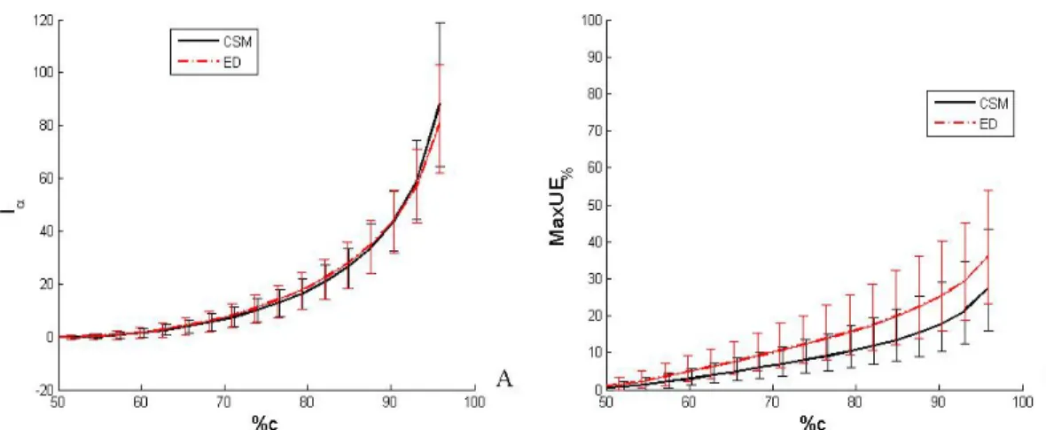
3-7 Average results for CSM and ED for Kriging based on 17 points.. . . 52
3-8 Average results for CSM and ED for PRS based on 17 points. . . 52
3-9 Average results for CSM and ED for Kriging based on 34 points.. . . 53
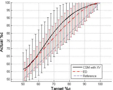
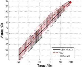
3-10 Target vs. actual %c for PRS using CSM with cross-validation and ED based on 17 points. . . 54
3-11 Target vs. actual %c for Kriging using CSM with cross-validation and ED based on 17 points. . . 55
3-12 Confidence intervals (CI) computed using classical regression and bootstrap when the error follows a lognormal distribution. . . 56
3-13 Average results for BS and ED for PRS based on 17 points. . . 57
3-14 Target vs. actual %c for Kriging using CSM and cross-validation and ED based on 17 points. . . 57
3-15 Average results for CSM (plain black) and ED (mixed grey) for PRS on the torque arm data. . . 59
3-16 Average results for CSM and ED for Kriging on the torque arm data. . . 59
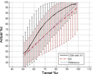
3-17 Target vs. actual %c for PRS using CSM and cross-validation and ED on the torque arm data. . . 60
3-18 Target vs. actual %c for Kriging using CSM and cross-validation and ED on
the torque arm data. . . 60
3-19 Average results for BS and ED for PRS on the torque arm data. . . 61
3-20 Target vs. actual %c for PRS using BS and ED on the torque arm data. . . . . 61
4-1 Criteria to fit empirical CDFs. . . 68
4-2 Example of CDF estimators based on RMS error for a sample of size 10 generated from N (−2.33, 1.02) . . . . 70
4-3 Conservative estimators of Pf from bootstrap distribution: 95th percentile (p95) and mean of the 10% highest values (CVaR).. . . 72
4-4 Mean and confidence intervals of the bootstrap p95 conservative estimators for Normal distribution. . . 77
4-5 Mean and confidence intervals of the bootstrap p95 conservative estimators for lognormal distribution. . . 77
4-6 Geometry and loading of the cryogenic laminate. . . 79
5-1 One-dimensional illustration of the target region. . . 91
5-2 Illustration of the weights functions. . . 95
5-3 Optimal design after 11 iterations. . . 102
5-4 Evolution of Kriging target contour line compared to actual during the sequential process. . . 103
5-5 Comparison of error distribution for the optimal and LHS DoEs. . . 105
5-6 Boxplots of errors for the LHS and optimal designs for the test points where responses are inside the domains [−σε, +σε . . . 106
5-7 Optimal designs with uniform integration measure and with input distribution integration measure. . . 107
6-1 Evolution of the response of the FEA for the torque arm example, when the complexity of the model (mesh density) increases. . . 113
6-2 D-optimal design for a second-order polynomial regression and corresponding prediction variance. . . 118
6-3 Full-factorial design with homogeneous allocation of computational effort and corresponding prediction variance.. . . 119
6-4 36-point Full-factorial design with homogeneous allocation of computational effort and corresponding prediction variance. . . 119
6-5 Evolution of the IMSE with respect to the number of observations for uniform
random designs with Gaussian and Exponential covariances. . . 123
6-6 Illustration of the MSE function for a Brownian motion (σ2 = 1, τ2 = 0.002). . . 127
6-7 Illustration of the MSE function for a Gaussian process (GP) with exponential covariance function (σ2 = 1, θ = 0.2 and τ2 = 0.002). . . . 129
6-8 Gears parameters definitions. . . 131
6-9 Optimum robust design found using the kriging metamodel. . . 132
A-1 Average results for Biased fitting with constraint relaxation and constraint selection on the Branin-Hoo function. . . 139
A-2 Average results for CSM and Biased fitting with constraint selection. . . 140
A-3 Average results for Indicator Kriging and ED with Kriging.. . . 142
A-4 Target vs. actual %c for IK (plain black) and Kriging with ED (mixed gray). . . 142
C-1 Representation of the function g (u) = 2uθ cos (u) + (1− θ2u2) sin (u). . . . 156
D-1 Gears parameters definitions. . . 159
D-2 Profile wear (mm) vs. angle (rad) . . . 161
D-3 ∆ST E without wear vs. ∆ST E with Archard’s wear profile (∆ST EA, A), and vs. the 90% percentile of ∆ST E with randomly perturbed Archard’s wear (B). . 167
D-4 ∆ST EA (with Archard’s wear profile) vs. ˆP∆ST E90 . . . 168
D-5 Example of an optimization run starting design. . . 170
D-6 Optimum design without wear . . . 170
D-7 Optimum robust design found using the kriging metamodel. . . 172
D-8 Optimum design with Archard’s wear. . . 173
D-9 Empirical MCS design, i.e., best design of the original latin hypercube set of points with 30 Monte Carlo simulations per point. . . 174
LIST OF ABBREVIATIONS BS Bootstrap
CDF Cumulative Distribution Function
CEC Conservative to the Empirical Curve
CSM Constant Safety Margin
CSP Conservative at Sample Points
DoE Design of Experiments
ED Error Distribution
eRM S Root Mean Square Error
lα Loss in accuracy
LHS Latin Hypercube Sampling
M axU E Maximum Unconservative Error
M axU E% Reduction of the Maximum Unconservative Error
MCS Monte-Carlo Simulations
MSE Mean Square Error
PDF Probability Density Function
Pf Probability of failure
PRS Polynomial Response Surface
RBDO Reliability-Based Design Optimization
Abstract of Dissertation Presented to the Graduate School of the University of Florida in Partial Fulfillment of the
Requirements for the Degree of Doctor of Philosophy
IMPROVING ACCURACY AND COMPENSATING FOR UNCERTAINTY IN SURROGATE MODELING
By Victor Picheny December 2009 Chair: Raphael T. Haftka
Major: Aerospace Engineering
In most engineering fields, numerical simulators are used to model complex
phenomena and obtain high-fidelity analysis. Despite the growth of computer capabilities, such simulators are limited by their computational cost. Surrogate modeling is a popular method to limit the computational expense. It consists of replacing the expensive model by a simpler model (surrogate) fitted to a few chosen simulations at a set of points called a design of experiments (DoE).
By definition, a surrogate model contains uncertainties, since it is an approximation to an unknown function. A surrogate inherits uncertainties from two main sources: uncertainty in the observations (when they are noisy), and uncertainty due to finite sample. One of the major challenges in surrogate modeling consists of controlling and compensating for these uncertainties. Two classical frameworks of surrogate application are used as a discussion thread for this research: constrained optimization and reliability analysis.
In this work, we propose alternatives to compensate for the surrogate model errors in order to obtain safe predictions with minimal impact on the accuracy. The methods are based on different error estimation techniques, some based on statistical assumptions and some that are non-parametric. Their efficiency are analyzed for general prediction and for the approximation of reliability measures.
We also propose two contributions to the field of design of experiments in order to minimize the uncertainty of surrogate models. Firstly, we address the issue of choosing the experiments when surrogates are used for reliability assessment and constrained optimization. Secondly, we propose global sampling strategies to answer the issue of allocating limited computational resource in the context of RBDO.
All methods are supported by quantitative results on simple numerical examples and engineering applications.
CHAPTER 1 INTRODUCTION
In the past decades, scientists have benefited from the development of numerical tools for the help of learning, prediction and design. The growth of computational capabilities has allowed the consideration of phenomena of constantly increasing level of complexity, which results in better understanding and more efficient solutions of real-life problems.
Complex numerical simulators can be encountered in a wide range of engineering fields. The automotive industry has developed numerical models for the behavior of cars during crash-tests, which involve highly non-linear mechanical modes, in order to integrate it to the design of car structures. In geophysics, flow simulators are used for the prediction of the behavior of CO2 sequestration into natural reservoirs, or the prediction of oil recovery enhancement, based on a complex mapping of ground characteristics.
The increasing computational power has also allowed the incorporation of uncertainty information into system analysis. In particular, reliability analysis aims at quantifying the chance that a system behaves as it is required, when a set of the problem parameters are uncertain [Rackwitz (2000), Haldar & Mahadevan (2000)]. In structural analysis, uncertainty typically comes from material properties (due to manufacturing) and actual working conditions. For obvious reasons, reliability assessment has been intensively explored in aerospace and nuclear engineering.
However, the gain in realism makes the use of numerical models extremely challenging. Indeed, the complexity of the simulators makes them highly expensive computationally, limiting systematic learning or design process. Also, the number of parameters (or input variables) that explain the phenomenon of interest can potentially be very large, making difficult the quantification of their influence on the simulator response.
To overcome computational cost limitations, surrogate models, or metamodels, have been frequently used on many applications. The idea of surrogate models consists of replacing the expensive model by a simpler mathematical model (or surrogate) fitted to a
few chosen simulations at a set of points called a design of experiments (DoE). Surrogate models are then used to predict the simulator response with very limited computational cost [Box & Draper (1986), Myers & Montgomery(1995), Santner et al. (2003),Sacks et al. (1989a)].
By definition, a surrogate model contains uncertainties, since it is an approximation to an unknown function. A surrogate inherits uncertainties from two main sources: uncertainty in the observations (when they are noisy), and uncertainty due to the lack of data. Indeed, a simulator is an approximation to a real phenomenon, and the confidence one can put in its responses depends on the quality of the numerical model. The properties of the surrogate strongly depend on the accuracy of the observations. Secondly, in most applications, the number of simulations runs is severely limited by the computational capabilities. The information on which the surrogate is fitted is insufficient to obtain an accurate approximation of the simulator behavior. One of the major challenges in surrogate modeling consists of controlling and compensating for these uncertainties.
The present work considers as a discussion thread the classical framework of reliability-based design optimization (RBDO), for which the issues associated with uncertainty in surrogate modeling are particularly crucial. RBDO is a popular way to address uncertainty in the design process of a system. It consists of optimizing a performance function while ensuring a prescribed reliability level. RBDO problems are computationally challenging, since they require numerous calls to reliability measures that are most of the time expensive to estimate, hence being a natural candidate for surrogate application [Rajashekhar & Ellingwood (1993), Venter et al. (1998),Kurtaran et al. (2002)]. Surrogate modeling can be used at two levels of the RBDO: (1) during the optimization process, by approximating the reliability constraint, and (2) during the reliability estimation itself.
The challenges in using surrogate modeling in RBDO are various. Indeed, a poor approximation of the reliability level can severely harm the optimization process: overestimation leads to non-optimal designs, and underestimation to weak designs. Reliability assessment methods are generally based on sampling methods (such as Monte-Carlo simulations) that only provide estimates of the actual reliability levels. Quantification of the uncertainty on both reliability estimates and a surrogate based on such data is needed to limit the risk of poor designs. Ramu et al. (2007) show that the use of surrogates for reliability assessment is particularly challenging, since small errors in the model could result in large errors in the reliability measure. In addition, for computational reasons, the number of reliability estimates is limited to a small value, and efficient
sampling strategies must be used to ensure an acceptable accuracy of the surrogate. It is possible to compensate for the lack of accuracy with extra safety margins. Such approach is often referred as conservative, and a conservativeness level quantify the chance that an approximation is on the safe side for the analysis. For example,
Starnes Jr & Haftka (1979) replaced the linear Taylor series approximation with a tangent approximation biased to be conservative in order to reduce the chance of unconservative approximations to buckling loads. Many engineering applications have adopted conservative estimation. For instance, Federal Aviation Administration (FAA) defines conservative material property (A-basis and B-basis) as the value of a material property exceeded by 99% (for A-basis, 90% for B-basis) of the population with 95% confidence. FAA recommends the use of A-basis for material properties and a safety factor of 1.5 on the loads. Traditionally, safety factors have been extensively used to account for uncertainties, even though their effectiveness is questionable [Elishakoff (2004),Acar et al.
(2007)].
Estimating the uncertainty in data or the metamodel is crucial for the effectiveness of most surrogate-based approaches. Uncertainty and error quantification is a classical theme of surrogate modeling. Most metamodels contain by construction error estimates [Cressie
(1993), Isaaks & Srivastava(1989), Box & Draper (1986)]. These estimates are based on statistical assumptions; for instance, linear regression assumes normality and independance of the errors. In practice, such assumptions can be violated, making those error measures questionable. Alternatively, numerical techniques are available to quantify the error [Stine
(1985), Efron(1982), Goel et al.(2006)].
Uncertainty quantification allows compensating mechanisms, for instance in order to set the conservativeness to a prescribed level. However, little information is available on the effect of error compensation on the surrogate application. Furthermore, conservative estimates are biased to be on the safe side, so the conservativeness comes at a price of accuracy. One goal of present work is to propose alternatives to compensate for the surrogate model errors, based on different error estimation techniques, and demonstrate their efficiency for safe prediction and design of engineering systems.
In many applications, sampling strategies can be chosen by the user. Then,
experiments can be designed such that the uncertainty of surrogate models are minimized. When safe prediction is desired, reduced uncertainty allows to obtain conservativeness with a minimal impact on accuracy. The choice and effectiveness of the sampling strategies has been widely explored and discussed in the surrogate literature [Steinberg & Hunter (1984), Sacks et al.(1989b), Fedorov & Hackl(1997)]. This work proposes two contributions to this field. Firstly, we address the issue of choosing the experiments when surrogates are used for reliability assessment and constrained optimization. Secondly, we propose global sampling strategies to answer the issue of allocating limited computational resource in the context of RBDO.
Outline of the dissertation:.
Chapter 2 reviews several aspects of surrogate modeling.
Chapter 3 addresses the issue of generating conservative predictions using surrogate models. Two alternatives are proposed: (1) using statistical information provided by the surrogate model and (2) using model-independent techniques (bootstrap, cross-validation)
to obtain statistical information. Different metrics are defined to measure the trade-off between accuracy and safety. The analysis of the different techniques is supported with the help of an analytical and a structural problem that uses finite elements analysis.
Chapter 4 considers the application of surrogate modeling to reliability-based design, where surrogates are used to fit probability distributions. We focus on the case when low probabilities are estimated from a small number of observations obtained by Monte-Carlo simulations (MCS). By using biased-fitting techniques and resampling methods (bootstrap), we compensate for the uncertainty in the analysis by being on the conservative side, with reasonable impact on the accuracy of the response. An
application to the optimization of a laminate composite with reliability constraints is used for demonstration, the constraint being approximated conservatively using bootstrap.
In Chapter 5, we propose an objective-based approach to surrogate modeling, based on the idea that the uncertainty may be reduced where it is most useful, instead of
globally. An original criterion is proposed to choose sequentially the design of experiments, when the surrogate needs to be accurate for certain levels of the simulator response. The criterion is a trade-off between the reduction of overall uncertainty in the surrogate, and the uncertainty reduction in target regions. The effectiveness of the method is illustrated on a simple reliability analysis application.
Chapter 6 considers the framework of simulators whose fidelity depends on tunable factors that control the complexity of the model (such as MCS-based simulators, or RBDO framework). For each simulation run, the user has to set a trade-off between computational cost and response precision. When a global computational budget for the DoE is given, one may have to answer the following questions: (1) is it better to run a few accurate simulations or a large number of inaccurate ones, (2) is it possible to improve the surrogate by tuning different fidelities for each run. Answers are proposed for these two questions. For polynomial regression, it joins the well-explored theory of design optimality.
For kriging, both numerical and analytical results are proposed; in particular, asymptotic results are given when the number of simulation runs tends to infinity.
Chapter 7 recapitulates major conclusions and results, and draw perspectives from this work.
CHAPTER 2
ELEMENTS OF SURROGATE MODELING
In this chapter, we introduce the important notions relative to surrogate modeling. We detail two types of models: linear regression models, and Kriging models. We also describe the problematic of design of experiments, and present several popular sampling strategies.
2.1 Surrogate Models
Strategies involving surrogate modeling are recognized in a wide range of engineering fields to efficiently address computationally expensive problems. The aim of this section is to briefly present the notation and main steps in surrogate modeling. Among the numerous types of surrogate models available in the literature, we emphasize two of the most popular ones: linear regression and Kriging. Linear regression, also referred as polynomial response surface in the engineering literature, has been initially developed for statistical inference based on physical experiments. Kriging was developed by geostatisticians to model spatial correlations of the physical characteristics of ground. Both models are now used in many applications, even though the hypotheses on which the models are based are not necessarily guaranteed.
A major notion in surrogate modeling is the design of experiments, or sampling strategy, since it is crucial to the quality of the surrogate analysis. In this chapter, we briefly describe three classical sampling strategies: space-filling, model-based designs and adaptive designs. More advanced notions are addressed in Chapter 5 for adaptive designs and Chapter 6 for model-oriented optimal designs.
2.1.1 Notation And Concepts
Let us first introduce some notation. We denote by y the response of a numerical simulator or function that is to be studied:
y : D⊂ Rd−→ R
x7−→ y(x)
where x = {x1, ..., xd}T is a d-dimensional vector of input variables, and D is the design
space. In order to build a metamodel, the response y is observed at n distinct locations X:
X = [x1, ..., xn]
Yobs = [y(x1), ..., y(xn)] T
= y(X)
(2–2)
X is called the design of experiments (DoE), and Yobs is the observations. Since the
response y is expensive to evaluate, we approximate it by a simple model, called the metamodel or surrogate model, based on assumptions on the nature of y and on its observations Yobs at the points of the DoE.
The metamodel can interpolate the data (splines, Kriging) or approximate it (linear regression, Kriging with nugget effect). In the latter case, it is assumed that the function of interest is observed through a noisy process, so the observation differs from the true function by an additive error term:
yobs,i = y(xi) + εi (2–3)
with εi the error. In most of the metamodel hypotheses, the error is considered as a white
noise normally distributed with zero mean. In this section, we will always consider this hypothesis true.
2.1.2 The Linear Regression Model
In linear regression, the response is modeled as a linear combination of basis functions observed with an additive error term:
y(x) = p ∑ j=1 βjfj(x) (2–4) yobs,i = p ∑ j=1 βjfj(x) + εi (2–5)
where fj(x) are the basis functions (for instance polynomial), βj the weights, and εi the
Given a set of design points, the linear regression model, in matrix notation, is defined as follow: Yobs = fT(X)β + ε (2–6) where: F = f(x1)T f(x2)T .. . f(xn)T β = β1 β2 .. . βp ε = ε1 ε2 .. . εp and: f(x)T = [ f1(x) f2(x) . . . fp(x) ] .
Typically, the fi can be chosen as polynomial functions; in that case the model is
often called polynomial response surface (PRS).
Since in practice the error is unknown, we estimate the response by:
ˆ
y(x) = f(x)Tβˆ (2–7)
where ˆβ is an estimate of β and is chosen by minimizing the mean square error (MSE)
between the estimates and the actual responses at all design points:
M SE = 1 n n ∑ i=1 [ˆy((xi))− y(xi)]2 (2–8)
Using the standard linear regression, the value of ˆβ that minimizes the MSE is given
by:
ˆ
β = (FTF)−1FTYobs (2–9) ˆ
β = M−1FTYobs (2–10)
The quantity M = FTF is called the Fisher information matrix.
In addition to the best predictor ˆy, the linear regression model provides a prediction variance, given by:
var [ˆy(x)] = f(x)TM−1f(x) (2–11)
When the error is heteroskedastic, that is, when the error distribution differ from one point to another, the ordinary least square estimator of β is not appropriate. Instead, we
estimate the coefficients by the generalized least square estimator β∗:
β∗ =(FTΓ−1F)−1FTΓ−1Yobs (2–12)
with: Γ = [cov (y(xi), y(xj))]1≤i,j≤n. In that case, the Fisher information matrix is:
M = FTΓ−1F (2–13)
Note that if the errors are uncorrelated, Γ reduces to diag [var(ε1), var(ε2), ..., var(εn)]. For calculation details, see for instance Box & Draper (1986),Khuri & Cornell (1996) orMyers & Montgomery (1995).
2.1.3 The Kriging Model
The Kriging metamodel was initially developed in the geostatistic framework
[Matheron(1969), Cressie (1993)] to predict values based on spatial correlation considerations. Kriging can also be found on the literature under the name of Gaussian Process regression [Rasmussen & Williams (2006)], or regression with spatially correlated errors [Fedorov & Hackl (1997)]. The main hypothesis behind the Kriging model is to assume that the true function y is one realization of a Gaussian stochastic process Y :
y(x) = Y (x, ω) (2–14)
where ω belongs to the underlying probability space Ω. In the following we use the notation Y (x) for the process and y(x) for one realization. For Universal Kriging, Y is of the form: Y (x) = p ∑ j=1 βjfj(x) + Z(x) (2–15)
where fj are linearly independent known functions, and Z is a Gaussian process with zero
mean and covariance k(u, v).
The covariance function (or kernel) k contains all the information of spatial dependency, and depends on parameters Θ. There exists many types of covariance functions; two of the most popular ones are the isotropic gaussian and exponential
covariances:
Isotropic Gaussian covariance: k(u, v) = σ2exp [ − ( ∥u − v∥ θ )2] (2–16)
Isotropic Exponential covariance: k(u, v) = σ2exp [ − ( ∥u − v∥ θ )] (2–17)
For these covariances, the parameters Θ are the process variance σ2 and range θ. Anisotropic covariance functions can also be defined by attributing a different θ in each direction:
Anisotropic Gaussian covariance: k(u, v) = σ2exp [ − d ∑ j=1 ( |uj− vj| θj )2] (2–18)
In Chapter 3, we also use the rational quadratic covariance function[Rasmussen & Williams (2006)]: k(u, v) = ( 1 + ∥u − v∥ 2 2αl2 )−α (2–19) with Θ ={α, l}.
In the geostatistic literature, three terminologies are used, depending on the linear part considered:
• simple Kriging (SK): the linear part reduces to a known constant β1 • ordinary Kriging (OK): the constant β1 is unknown
• universal Kriging (UK) is the general case.
The parameters Θ are usually unknown and must be estimated based on the observations, using maximum likelihood, cross-validation or variogram techniques for instance [see Rasmussen & Williams (2006),Stein (1999) or Cressie (1993)]. However, in the Kriging model they are considered as known. To account for additional variability due to the parameter estimation, one may use Bayesian Kriging models [see Martin & Simpson (2004) and Oakley & O’Hagan (2004)], which will not be detailed here.
2.1.3.1 Kriging with noise-free observations
First, we consider the most classical framework, where the function is observed without noise:
yobs,i = y(xi) (2–20)
Under such hypothesis, the best linear unbiased predictor (BLUP) for y, knowing the observations Yobs, is given by the following equation:
mK(x) = E [Y (x)|Y (X) = Yobs] = f(x)Tβ + c(x)ˆ TC−1 ( Yobs− F ˆβ ) (2–21) where: • f(x) =[f1(x) . . . fp(x) ]T is p× 1 vector of bases, • β =ˆ [βˆ 1 . . . βˆp ]T is p× 1 vector of estimates of β, • c(x) =[cov(x, x1) . . . cov(x, xn) ]T is n× 1 vector of covariance, • C = [cov (xi, xj)]1≤i,j≤n is n× n covariance matrix, and
• F =[f(x1) . . . f(xn)
]T
is p× n matrix of bases.
ˆ
β is the vector of generalized least square estimates of β:
ˆ
β =(FTC−1F)−1FTC−1Yobs (2–22)
In addition, the Kriging model provides an estimate of the accuracy of the mean predictor, the Kriging prediction variance:
s2K(x) = k(x, x)−c(x)TC−1c(x)+(f(x)T − c(x)TC−1F) (FTC−1F)−1(f(x)T − c(x)TC−1F)T
(2–23) Note that the Kriging variance does not depend on the observations Yobs, but only on the
design of experiments. Derivation details can be found inMatheron (1969),Cressie (1993), orRasmussen & Williams (2006). We denote by M(x) the Gaussian process conditional on
the observations Yobs:
(M (x))x∈D = (Y (x)|Y (X) = Yobs)x∈D = (Y (x)|obs)x∈D (2–24)
The Kriging model provides the distribution of M at a prediction point x:
M (x)∼ N(mK(x), s2K(x)
)
(2–25)
Figure2-1 shows a Kriging model with a first-order trend (β = β1, simple Kriging) and five equally-spaced observations along with the 95% confidence intervals, which are calculated from mK± 1.96sK. On this example, the confidence interval contains the actual
response.
Figure 2-1. Example of Simple Kriging model. The 95% confidence intervals (CI) are equal to mK ± 1.96 × sK. The DoE consists of five points equally spaced in [0, 1].
The Kriging mean mK interpolates the function y(x) at the design of experiment
points:
mK(xi) = y(xi), 1 ≤ i ≤ n (2–26)
The Kriging variance is null at the observation points xi, and greater than zero
elsewhere:
Besides, the Kriging variance function increases with the distance of x to the observations.
2.1.3.2 Kriging with nugget effect
When noisy observations are considered, a diagonal matrix must be added to the covariance matrix:
C∆ = C + ∆ (2–28)
with: ∆ = diag ([var(ε1), var(ε2), . . . , var(εn)]) the variances of the observations.
Equations for mK and s2K are the same as in Eqs. 2–21 and 2–23 but using C∆
instead of C. For theoretical details and bibliography, see for instanceGinsbourger (2009) (Chap. 7). The main difference with the classical Kriging is that best predictor is not an interpolator anymore; also, the Kriging variance is non-null at the observation points. Figure2-2 shows a Kriging model based on noisy observations. Each observation has a different noise variance.
Figure 2-2. Example of Simple Kriging model with noisy observations. The bars represent ± two times the standard deviation of the noise. The Kriging mean does not interpolate the data and the Kriging variance is non-null at the observation points.
2.2 Design Of Experiment Strategies
Choosing the set of experiments X plays a critical role in the accuracy of the
metamodel and the subsequent use of the metamodel for prediction, learning or optimization. In this section, we detail three families of design of experiments: classical and space-filling designs, model-oriented (or optimal) designs, and adaptive designs.
2.2.1 Classical And Space-Filling Designs
The first family of DoE consists of designs based on geometric considerations. In a full-factorial (FF) design, the variables are discretized into a finite number of levels, and the design consists of all the possible combinations of the discrete variables. Two-level FF designs, where the input variables are taken only at their minimum and maximum values, are typically used for screening in order to identify the most significant variables and remove the others. Although extensively used historically, such type of DoEs suffer from several drawbacks among the following:
• it requires a large number of observations in high dimensions (a FF design with q levels in d dimensions is made of qd observations), making them impractical for
computationally expensive problems
• they do not ensure space-filling in high dimensions
• the number of observation points collapses when projecting on the subspaces (when some variables are removed for instance).
Figure 2-3. Examples of full-factorial and central composite designs.
There exists classical alternatives to FF designs, such as central-composite designs (that consist of 2d vertices, 2d axial points and p repetitions of central point), or fractional
designs (that are subsets of FF designs). See for instance Myers & Montgomery (1995) for details. Figure 2-3 shows a three-level FF design and a central composite design for a two-dimensional domain.
A popular alternative to the geometrical designs is Latin Hypercube sampling (LHS) [McKay et al. (2000)]. LHS is a random DoE that insures uniformity of the marginal distributions of the input variables.
To generate a DoE of n points, each variable range is divided into n equal intervals, for instance for the range [0, 1]: {[0,1n], [1n,2n], ..., [n−1n , 1]}. Then, the DoE is constructed by picking n points so that all the intervals for each variable is represented once. Figure
2-4 shows a nine-point LHS design for a two-dimensional domain. In a d-dimensional space, the total number of combinations is nd−1, which increases very rapidly with both
sample size and dimension. The variable values can be chosen deterministically as the centre of the interval for instance, or randomly inside the interval.
LHS can also be optimized to ensure better space-filling. Space-filling criteria include: • maximum minimum distance between sampling points (maximin designs),
• maximum-entropy designs [Shewry & Wynn (1987)], • minimum discrepancy measures, etc.
Figure 2-4. A nine-point LHS design. The projections on the margins are non redudant and equally-spaced if the design points are centered in each cell.
Finally, low-discrepancy sequences are also often used for space-filling strategies, such as Sobol, Halton, Harmmersley, Niederreitter or Faure sequences. See Niederreiter (1992) orSobol (1976) for details.
2.2.2 Model-Oriented Designs
The previous sampling strategies were built independently of the metamodel to be fitted to the observations. Alternatively, when the choice of the metamodel is made a priori, it is possible to choose the observation points in order to maximize the quality of statistical inference. The theory of optimal designs has originally been developed in the framework of linear regression, and was extended later to other models such as Kriging since the 80’s.
Let ϕ be a functional of interest to minimize that depends on the design of experiments
X. A design X∗ is called ϕ-optimal if it achieves:
X∗ = argmin [ϕ(X)] (2–29)
A- and D-optimality aim at minimizing the uncertainty in the parameters of the metamodel when uncertainty is due to noisy observations. In the framework of linear regression, D-optimal designs minimize the volume of the confidence ellipsoid of the coefficients, while A-optimal designs minimize its perimeter (or surface for d > 2). Formally, the A- and D-optimality criteria are, respectively, the trace and determinant of Fisher’s information matrix [Khuri & Cornell (1996)]:
A(X) = trace(M (X)) (2–30)
D(X) = det(M (X)) (2–31)
In linear regression, these criteria are particularly relevant since minimizing the uncertainty in the coefficients also minimizes the uncertainty in the prediction (according to the D-G equivalence theorem, which is developed further in Chapter 6).
For Kriging, uncertainties in covariance parameters and prediction are not simply related. A natural alternative is to take advantage of the prediction variance associated with the metamodel. The prediction variance allows us to build measures that reflect the overall accuracy of the Kriging. Two different criteria are available: the integrated mean square error (IMSE) and maximum mean square error (MMSE) [Santner et al. (2003),
Sacks et al. (1989a)]:
IM SE = ∫
D
M SE(x)dµ(x) (2–32)
M M SE = maxx∈D[M SE(x)] (2–33)
µ(x) is an integration measure (usually uniform) and
M SE(x) = E[(y(x)− M(x))2 obs] (2–34) When the function to approximate is a realization of a gaussian process with
covariance structure and parameters equal to the ones chosen for Kriging, the MSE coincides with the prediction variance s2
K. Note that the above criteria are often called
I-criterion and G-criterion, respectively, in the regression framework. The IMSE is a measure of the average accuracy of the metamodel, while the MMSE measures the risk of large error in prediction. In practice, the IMSE criterion essentially reflects the spatial distribution of the observations. For dimensions higher than two, the MMSE is not very relevant since the regions of maximum uncertainty are always situated on the boundaries, and MMSE-optimal designs consist of observations taken on the edges of the domain only, which is not efficient for Kriging.
Optimal designs are model-dependent, in the sense that the optimality criterion is determined by the choice of the metamodel. In regression, A- and D-criteria depend on the choice of the basis functions, while in Kriging the prediction variance depends on the linear trend, the covariance structure, and parameter values. A fundamental result, however, is that assuming a particular model structure (and covariance parameters for
Kriging), none of the criteria depends on the response values at the design points. The consequence is that the DoEs can be designed offline before generating the observations. However, in practice this statement has to been moderated, since the Kriging covariance parameters are most of the time estimated from the observations.
2.2.3 Adaptive Designs
The previous DoE strategies choose all the points of the design before computing any observation. It is also possible to build the DoE sequentially, by choosing a new point as a function of the other points and their corresponding response values. Such approach has received considerable attention from the engineering and mathematical statistic communities, for its advantages of flexibility and adaptability over other methods [Lin et al. (2008),Scheidt (2006), Turner et al. (2003)].
Typically, the new point achieves a maximum on some criterion. For instance, a sequential DoE can be built by making at each step a new observation where the prediction variance is maximal. The algorithmic procedure is detailed in Table 2-1. Table 2-1. Sequential DoE minimizing the maximum prediction variance at each step.
X ={x1, . . . , xn} for i = 1 to k
xnew = arg max x∈D
s2K(x)
X ={X, xnew} end
Sacks et al. (1989b) uses this strategy as a heuristic to build IMSE-optimal designs for Kriging. Theoretically, this sequential strategy is less efficient that the direct minimization of the IM SE criterion. The advantage of sequential strategy here is twofold. Firstly, it is computational, since it transforms an optimization problem of dimension n× d (for the IMSE minimization) into k optimizations of dimension d. Secondly, it allows us to reevaluate the covariance parameters after each observation. In the same fashion, Williams et al. (2000),Currin et al. (1991),Santner et al. (2003) use a Bayesian approach to derive sequential IMSE designs. Osio & Amon(1996) proposed a multistage approach to enhance
first space-filling in order to accurately estimate the Kriging covariance parameters and then refine the DoE by reducing the model uncertainty. Some reviews of adaptive sampling in engineering design can be found in Jin et al.(2002).
In general, a particular advantage of sequential strategies over other DoEs is that they can integrate the information given by the first k observation values to choose the (k + 1)th
training point, for instance by reevaluating the Kriging covariance parameters. It is also possible to define response-dependent criteria, with naturally leads to surrogate-based optimization. One of the most famous adaptive strategy is the EGO algorithm (Jones et al. (1998)), used to derive sequential designs for the optimization of deterministic simulation models. At each step, the new observation is chosen to maximize the expected improvement, a functional that represents a compromise between exploration of unknown regions and local search:
EI (x) = E (max [0, min (Yobs)− M (x)]) (2–35)
where M (x) is the Kriging model as described in Eq. 2–25.
Kleijnen & Van Beers (2004) proposed an application-driven adaptive strategy using criteria based on response values. Tu & Barton(1997) used a modified D-optimal strategy for boundary-focused polynomial regression. In Chapter 5, we detail an original adaptive design strategy for target region approximation.
CHAPTER 3
CONSERVATIVE PREDICTIONS USING SURROGATE MODELING
3.1 Motivation
In analyzing engineering systems, multiple sources of error - such as modeling error or insufficient data - prevent us from taking the analysis results at face value. Conservative prediction is a simple way to account for uncertainties and errors in a system analysis, by using calculations or approximations that tend to safely estimate the response of a system. Traditionally, safety factors have been extensively used for that purpose, even though their effectiveness is questionable [Elishakoff (2004),Acar et al. (2007)].
When surrogate models are used for predicting critical quantities, very little is known in practice to provide conservative estimates, and how conservative strategies impact the design process. Most surrogates are designed so that there is a 50% chance that the prediction will be higher than the real value. The objective of this work is to propose alternatives to modify the traditional surrogates so that this percentage is pushed to the conservative side with the least impact on accuracy.
Since conservative surrogates tend to overestimate the actual response, there is a trade-off between accuracy and conservativeness. The choice of such trade-off determines the balance between the risk of overdesign and the risk of weak design. The design of conservative surrogates can be considered as a bi-objective optimization problem, and results are presented in the form of Pareto fronts: accuracy versus conservativeness.
The most classical conservative strategy is to bias the prediction response by a multiplicative or additive constant. Such approaches are called empirical because the choice of the constant is somehow arbitrary and based on previous knowledge of the engineering problem considered. However, it is difficult to predict how efficient its application is to surrogates, and how it is possible to design those quantities. Alternatively, it is possible to use the statistical knowledge from the surrogate fitting (prediction variance) to build one-sided confidence intervals on the prediction.
For this study, we consider two types of surrogate models: polynomial response surfaces (PRS) and Kriging. We propose three alternatives to provide conservative estimates: using cross-validation to define constant margins, using confidence intervals given by the surrogate model, and using the bootstrap method. The methods differ in the sense that one assumes a particular distribution of the error, while the others (cross-validation and bootstrap) does not. Different metrics are defined to analyze the trade-off between accuracy and conservativeness. The methods are applied to two test problems: one analytical and one based on Finite Element Analysis.
3.2 Design Of Conservative Predictors 3.2.1 Definition Of Conservative Predictors
Without any loss of generality, we assume here that a conservative estimator is an estimator that does not underestimate the actual value. Hence, a conservative estimators can be obtained by simply adding a positive safety margin to the unbiased estimator:
ˆ
ySM(x) = ˆy (x) + Sm (3–1)
Alternatively, it is possible to define a conservative estimator using safety factors, which are more commonly used in engineering:
ˆ
ySF (x) = ˆy (x)× Sf (3–2)
In the context of surrogate modeling, safety margins are more convenient. Indeed, when using a safety factor, the level of safety depends on the response value, while most surrogates model assume that the error is independent of the mean of the response. Hence, in this work we use only safety margins to define a conservative estimator.
The value of the margin directly impacts the level of safety and the error in the estimation. Hence, there is a great incentive to find the margin that ensure a targeted level of safety with least impact on the accuracy of the estimates. The safety margin can be constant, or depend on the location, hence written Sm(x) (pointwise margin). In the
following sections, we provide several ways to design the margin, using parametric and non-parametric methods, for pointwise and constant margins.
3.2.2 Metrics For Conservativeness And Accuracy
As discussed in introduction, conservative estimates are biased, and a high level of conservativeness can only be achieved at a price in accuracy. Thus, the quality of a method can only be measured as a trade-off between conservativeness and accuracy. In order to assess a global performance of the methods, we propose to define accuracy and conservativeness indexes.
The most widely used measure to check the accuracy of a surrogate is the root mean square error (eRM S), defined as:
eRM S = ∫ D (ˆy (x)− y (x))2dx 1 2 (3–3)
The eRM S can be computed by Monte-Carlo integration at a large number of ptest test
points: eRM S ≈ v u u t 1 ptest ptest ∑ i=1 e2 i (3–4)
where ei = (ˆyi − yi), ˆyi and yi being the values of the conservative prediction and
actual simulation at the i-th test point, respectively.
We also define the relative loss in accuracy, in order to measure simply by how much the accuracy is degraded when high levels of conservativeness are targeted:
lα=
eRM S
eRM S|ref
− 1 (3–5)
where eRM S is taken at a given target conservativeness; and eRM S|ref is the eRM S
value of reference. In most of the study, which we take equal to the value of eRM S when
There are different measures of the conservativeness of an approximation. Here we use the percentage of conservative errors (i.e. positive):
%c = 100 ∫
D
I [ˆy (x)− y (x)]dx (3–6) where I(e) is the indicator function, which equals 1 if e > 0 and 0 otherwise. %c can be estimated by Monte-Carlo integration:
%c≈ 100 ptest
p∑test i=1
I (ei) (3–7)
Ideally, for most surrogate models, %c = 50% when the approximation is unbiased. The percentage of conservative errors provides the probability to be conservative. However, it fails to inform by how much it is unconservative when predictions are unconservative. Thus, an alternate measure of conservativeness is proposed; that is, the maximum unconservative error (largest negative error) :
MaxUE = max (max (−ei) , 0) (3–8)
This index can also be normalized by the index of the unbiased estimator:
MaxUE%=
MaxUE
MaxUE|ref − 1 (3–9) where MaxUE|ref is the value of reference, which we take equal to the value for the unbiased estimator.
A value of MaxUE% of 50% means that the maximum unconservative error is reduced by 50% compared to the BLUE estimator.
Alternative measures of conservativeness can be defined, including the mean or the median of the unconservative errors. However, the maximum error decreases monotonically when target conservativeness is increased, while mean and median can increase when we increase conservativeness, for instance when we have initially very small and very large errors.
3.2.3 Constant Safety Margin Using Cross-Validation Techniques
Here, we consider the design of conservative surrogates, when the same safety margin is applied everywhere on the design domain. In the following, we call such estimators CSM estimators (for Constant Safety Margin), and denote it ˆyCSM.
In terms of the cumulative distribution function (CDF) of the errors, Fe, the safety
margin Sm for a given conservativeness, %c, is given as:
Sm = Fe−1 ( %c 100 ) (3–10)
The objective is to design the safety margin such that the above equation is ensured. The actual error distribution is, in practice, unknown. We propose here to estimate it empirically using cross-validation techniques in order to choose the margin.
Cross-validation (XV) is a process of estimating errors by constructing the surrogate without some of the points and calculating the errors at these left out points. The process is repeated with different sets of left-out points in order to get statistically significant estimates of errors. The process proceeds by dividing the set of n data points into subsets. The surrogate is fitted to all subsets except one, and error is checked in the subset that was left out. This process is repeated for all subsets to produce a vector of cross-validation errors, eXV. Usually, only one point is removed at a time (leave-one-out cross-validation),
so the size of eXV is equal to n.
The empirical CDF FXV, defined by the n values of eXV, are an approximation of the
true distribution Fe. Now, in order to design the margin, we replace Fe in Eq. 3–10 by
FXV: Sm = FXV−1 ( %c 100 ) (3–11)
For instance, when n = 100 and 75% conservativeness is desired, the safety margin is chosen equal to the 25th highest cross-validation error.