HAL Id: hal-01093776
https://hal.inria.fr/hal-01093776
Submitted on 12 Dec 2014
HAL is a multi-disciplinary open access
archive for the deposit and dissemination of
sci-entific research documents, whether they are
pub-lished or not. The documents may come from
teaching and research institutions in France or
abroad, or from public or private research centers.
L’archive ouverte pluridisciplinaire HAL, est
destinée au dépôt et à la diffusion de documents
scientifiques de niveau recherche, publiés ou non,
émanant des établissements d’enseignement et de
recherche français ou étrangers, des laboratoires
publics ou privés.
Exact Protein Structure Classification Using the
Maximum Contact Map Overlap Metric
Inken Wohlers, Mathilde Le Boudic-Jamin, Hristo Djidjev, Gunnar W. Klau,
Rumen Andonov
To cite this version:
Inken Wohlers, Mathilde Le Boudic-Jamin, Hristo Djidjev, Gunnar W. Klau, Rumen Andonov. Exact
Protein Structure Classification Using the Maximum Contact Map Overlap Metric. [Research
Re-port] INRIA Rennes - Bretagne Atlantique and University of Rennes 1, France; Genome Informatics,
University of Duisburg-Essen, Germany; Life Sciences, CWI, Science Park 123, 1098 XG
Amster-dam, The Netherlands; Los Alamos National Laboratory, Los Alamos, NM, USA. 2014, pp.262 - 273.
�hal-01093776�
maximum contact map overlap metric
Inken Wohlers1, Mathilde Le Boudic-Jamin2, Hristo Djidjev4,
Gunnar W. Klau3, and Rumen Andonov2
1
Genome Informatics, University of Duisburg-Essen, Germany,
2 INRIA Rennes - Bretagne Atlantique and University of Rennes 1, France, 3
Life Sciences, CWI, Science Park 123, 1098 XG Amsterdam, The Netherlands,
4
Los Alamos National Laboratory, Los Alamos, NM, USA
Abstract. In this work we propose a new distance measure for compar-ing two protein structures based on their contact map representations. We show that our novel measure, which we refer to as the maximum contact map overlap (max-CMO) metric, satisfies all properties of a metric on the space of protein representations. Having a metric in that space allows to avoid pairwise comparisons on the entire database and thus to significantly accelerate exploring the protein space compared to no-metric spaces. We show on a small gold-standard superfamily classification benchmark set of 6, 759 proteins that our exact scheme classifies up to 224 out of 236 queries correctly and on an larger, extended version of the benchmark up to 1361 out of 1369 queries. Our k-NN classification thus provides a promising approach for the automatic classification of protein structures into SCOP or CATH based on flexible contact map overlap alignments.
1
Introduction
Understanding the functional role and evolutionary relationships of proteins is key to answering many important biological and biomedical questions. Because the function of a protein is determined by its structure and because structural properties are usually conserved throughout evolution, such problems can be better approached if proteins are compared based on their representations as three-dimensional structures rather than as sequences. Databases such as SCOP [15] and CATH [16] have been built to organize the space of protein structures. Both SCOP and CATH, however, are constructed based on manual curation, and many of the currently over 90, 000 protein structures in the protein data bank (PDB) [3] are still unclassified. Moreover, classifying a newly found structure manually is both expensive in terms of human labor and slow. Therefore, computational methods that can accurately and efficiently complete such classifications will be highly beneficial. Basically, given a query protein structure, the problem is to find its place in a classification hierarchy of structures, for example, to predict its family or superfamily in the SCOP database.
One approach to solving that problem is based on having introduced a meaningful distance measure between any two protein structures. Then the family of a query protein q can be determined by comparing the distances between q and members of candidate families and choosing a family whose members are “closer” to q than members of the other families, where the precise criteria for deciding which family is closer depend on the specific implementation. But the key condition and a crucial factor for the quality of the classification result is having an appropriate distance measure between proteins.
Several such distances have been proposed, each having its own advantages. Recently, a number of approaches based on a graph-based measure of closeness called contact map overlap (CMO) [7] have been shown to perform well [2, 4, 11, 12, 17, 19, 20]. Informally, CMO corresponds to the maximum size of a common subgraph of the two contact map graphs, see the next section for the formal definition. Although CMO is a widely used measure, none of the CMO-based distance methods suggested so far satisfy the triangle inequality and, hence, introduce a metric on the space of protein representations. Having a metric in that space establishes a structure that allows much faster exploration of the space compared to no-metric spaces. For instance, all previous CMO-based algorithms require pairwise comparisons on the entire database, which takes time quadratic to the size of the database. With the rapid increase of the protein databases, such a strategy will unavoidably create performance problems even if the individual comparisons are fast. On the other hand, as we show here, the structure introduced in metric spaces can be exploited to significantly reduce the number of needed comparisons for a query and thereby increase the efficiency of the algorithm, without sacrificing the accuracy of the classification.
In this work we propose a new distance measure for comparing two protein structures based on their contact map representations. We show that our novel measure, which we refer to as the maximum contact map overlap (max-CMO) metric, satisfies all properties of a metric. The advantages of nearest-neighbor searching in metric spaces are well described in the literature [5, 13, 14]. We use max-CMO in combination with an exact approach for computing the CMO between a pair of proteins in order to classify protein structures accurately and efficiently in practice. Specifically, we classify a protein structure according to the k nearest neighbors with respect to the max-CMO metric. We demonstrate that one can speed-up the total time taken for CMO computations by computing in many cases approximations of CMO in terms of lower-bound upper bound intervals, without sacrificing accuracy. We point out that our approach solves the classification problem to provable optimality and that we do so without having to compute all alignments to optimality. We show on a small gold-standard superfamily classification benchmark set of 6, 759 proteins that our exact scheme classifies up to 224 out of 236 queries correctly and on a large, extended version of the data set that contains 67, 609 proteins even up to 1361 out of 1369. Our k-NN classification thus provides a promising approach for the automatic classification of protein structures into SCOP or CATH based on flexible contact map overlap alignments.
Amongst the other existing (non-CMO) protein structures comparison methods we are aware of only one exploiting the triangle inequality. This is the so called scaled Gauss metric (SGM) introduced in [18] and further developed in [9]. As shown in the above papers, their approach is very successful for automatic classification. In this work, however, we focus on contact map overlap and a comparison to classification algorithms based on different concepts is outside the scope of this paper.
2
The maximum contact map overlap metric
We introduce here the notions of contact map overlap (CMO) and the related max-CMO distance between protein structures. A contact map describes the structure of a protein P in terms of a simple, undirected graph G = (V, E) with vertex set V and edge set E. The vertices of V are linearly ordered and correspond to the sequence of residues of P . Edges denote residue contacts, that is, pairs of residues that are close to each other. More precisely, there is an edge (i, j) between residues i and j iff the Euclidean distance in the protein fold is smaller than a given threshold. The size |G| := |E| of a contact map is the number of its contacts. Given two contact maps G1(V, E1) and G2(U, E2) for two
protein structures, let I = (i1, i2, . . . , im) and J = (j1, j2, . . . , jm) be subsets of
V and U , respectively, respecting the linear order. Vertex sets I and J encode an alignment of G1and G2in the sense that vertex i1 is aligned to j1, i2to j2 and
so on. In other words, the alignment (I, J ), is a one-to-one mapping between the sets V and U . Given an alignment (I, J ), a shared contact (or common edge) occurs if both (ik, il) ∈ E1 and (jk, jl) ∈ E2 exist. We say in this case that
the shared contact (ik, il) is activated by the alignment (I, J ). The maximum
contact overlap problem consists in finding an alignment (I∗, J∗) that maximizes the number of shared contacts and CMO(G1, G2) denotes then this maximum
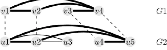
number of shared contacts between the contact maps G1and G2, see Figure 1.
v1 v2 v3 v4
u1 u2 u3 u4 u5
G1
G2
Fig. 1. The alignment visualized with dashed lines ((v1 ↔ u1)(v2 ↔ u2)(v3 ↔
u4)(v4 ↔ u5)) maximizes the number of the common edges between the graphs G1
and G2. The alignment activates four common edges that are emphasized in bold (i.e.,
CMO(G1, G2) = 4).
Computing CMO(G1, G2) is NP-hard [8]. Nevertheless, maximum contact
map overlap has been shown to be a meaningful way for comparing two protein structures [2,4,11,12,17,19,20]. Previously, several distances have been proposed
based on the maximum contact map overlap, for example, Dmin [4, 10, 17] and Dsum[2, 12, 17, 20] with Dmin(G1, G2) = 1 − CMO(G1, G2) min{|E1|, |E2|} and Dsum(G1, G2) = 1 − 2CMO(G1, G2) |E1| + |E1| . These distances have the disadvantage that they are no metrics as the following lemma shows.
Lemma 1. Distances Dmin and Dsum do not satisfy the triangle inequality.
Proof. See the counterexample in Fig. 2 below.
v1 v2 v3 v4 v5 v6 u1 u2 u3 u4 u5 u6 w1 w2 w3 w4 w5 w6 x1 x2 x3 x4 x5 x6 G1 G2 G3 G4
Fig. 2. Consider graphs G1, . . . , G4. It is easily seen that CMO(G1, G2) =
1, CMO(G2, G3) = 3 and CMO(G1, G3) = 3. We then obtain: Dsum(G1, G2) =
1 −|E 2 1|+|E2| = 1 − 2 6 = 2 3, Dsum(G2, G3) = 1 − 6 |E2|+|E3| = 1 − 6 8 = 1 4, Dsum(G1, G3) = 1 − 6 |E1|+|E3| = 1 − 6 8 = 1
4. Hence Dsum(G1, G3) + Dsum(G3, G2) = 1 2 <
2 3 =
Dsum(G1, G2). Furthermore, CMO(G2, G4) = 1 and CMO(G3, G4) = 2. We then
obtain: Dmin(G2, G4) = 1 −min{|E1CMO(G2,G4)|,|E 4|} = 1 − 1 3 = 2 3 and Dmin(G3, G4) = 1 − 2 3 = 1 3,
as well as Dmin(G2, G3) = 1 −33 = 0. Hence, Dmin(G2, G3) + Dmin(G3, G4) = 0 +13 < 2
3 = Dmin(G2, G4).
Let G1(V, E1), G2(U, E2) be two contact maps graphs. We propose a new
distance
Dmax(G1, G2) = 1 −
CMO(G1, G2)
max{|E1|, |E2|}
. (1)
The following claim states that Dmax is indeed a distance (metric) on the
space of contact maps and we refer to it as the max-CMO metric. Lemma 2. Dmax is a metric on the space of contact maps.
Proof. To prove the triangle inequality for the function Dmax, we consider three
contact maps G1(V, E1), G2(U, E2), G3(W, E3), and we want to prove that
Dmax(G1, G2) + Dmax(G2, G3) ≥ Dmax(G1, G3). We will use the fact that a
similar function dmaxon sets is a metric, which is defined as
dmax(A, B) = 1 −
|A ∩ B|
The mapping M corresponding to CMO(G1, G2) generates an alignment
(V0, U0), where V0 ⊆ V and U0 ⊆ U are ordered sets of vertices preserving the order of V and U , correspondingly. Since M is a one-to-one mapping, we can rename the vertices of U0 to the names of the corresponding vertices of V0 and keep the old names of the vertices of U \ U0. Denote the resulting ordered vertex set by U and denote by E2 the corresponding set of edges. Define the
graph G2= (U , E2). Note that |E2| = |E2| and any common edge discovered by
CMO(G1, G2) has the same endpoints (after renaming) in E2 as in E1; hence
CMO(G1, G2) = CMO(G1, G2) = |E1∩ E2|. Then from (2)
Dmax(G1, G2) = 1 − CMO(G1, G2) max{|E1|, |E2|} = 1 − |E1∩ E2| max{|E1|, |E2|} = dmax(E1, E2) .
Similarly, we compute the mapping corresponding to CMO(G2, G3) and generate
an optimal alignment (U0, W0). As before, we use the mapping to rename the vertices of W0 to the corresponding vertices of U0
and denote the resulting sets of vertices and edges by W and E3. Similarly to the above case, it follows that
Dmax(G2, G3) = dmax(E2, E3). Combining the last two equalities, we get
Dmax(G1, G2) + Dmax(G2, G3) = dmax(E1, E2) + dmax(E2, E3)
≥ dmax(E1, E3). (3)
On the other hand, E1∩ E3 contains only edges jointly activated by the
align-ments (V0, U0) and (U0, W0) and its cardinality is not larger than CMO(G1, G3),
which corresponds to the optimal alignment between G1 and G3. Hence
|E1∩ E3| ≤ CMO(G1, G3) and, since |E3| = |E3|,
dmax(E1, E3) = 1 − |E1∩ E3| max{|E1|, |E3|} ≥ 1 − CMO(G1, G3) max{|E1|, |E3|} = Dmax(G1, G3).
Combining the last inequality with (3) proves the triangle inequality for Dmax.
The other two properties of a metric, that Dmax(G1, G2) ≥ 0 with equality if and
only if G1= G2and Dmax(G1, G2) = Dmax(G2, G1), are obviously also true. ut
If instead of CMO(G1, G2) one computes lower or upper bounds for its
value, replacing those values in (1) produces an upper or lower bound for Dmax,
respectively.
3
Nearest neighbor classification of protein structures
We suggest to approach the problem of classifying a given query protein structure with respect to a database of target structures based on a majority vote of the k nearest neighbors in the database. Nearest neighbor classification is a simple and popular machine learning strategy with strong consistency results, see for example [1].
An important feature of our approach is that it is based on a metric and we fully profit from all usual benefits when exploiting the structure introduced by that metric. In addition, we also model each protein family in the database as a ball with a specially chosen protein from the family as center, see Sect. 3.1 for details. This allows to obtain upper and lower bounds for the max-CMO distance in Sect. 3.2, which are used to define a new dominance rule we call triangle dominance that proves to be very efficient. Finally, we describe in Sect. 3.3 how these results can be used in a classification algorithm.
3.1 Finding superfamily representatives
In order to minimize the number of targets with which a query has to be compared directly, i.e., via computing an alignment, we designate a representative central structure for each family. Let d denote any metric. Each family F ∈ C can then be characterized by a representative structure RF and a
family radius rF determined by
RF = arg min
A∈F maxB∈F d(A, B), rF = minA∈F maxB∈F d(A, B). (4)
In order to find RF and rF, we compute, during a preprocessing step, all
pairwise distances within F . We aim to compute these distances as precise as possible, using a sufficiently long run time for each pairwise comparison. Since proteins from the same family are structurally similar, the alignment algorithm performs favorably and we can usually compute inter-family distances optimally. 3.2 Dominance between target protein structures
In order to find the target structures which are closest to a query q, we have to decide for a pair of targets A and B which one is closer. We call such a relationship between two target structures dominance:
Definition 1 (dominance). Protein A dominates protein B with respect to a query q if and only if d(q, A) < d(q, B).
In order to conclude that A is closer to q than B, it may not be necessary to know d(q, A) and d(q, B) exactly. It is sufficient that A directly dominates B according to the following rule.
Lemma 3 (direct dominance). Protein A dominates protein B with respect to a query q if d(q, A) < d(q, B), where d(q, A) and d(q, B) are an upper and lower bound on d(q, A) and d(q, B), respectively.
Proof. Follows from the inequalities d(q, A) ≤ d(q, A) < d(q, B) ≤ d(q, B). ut Given a query q, a representative r and a target A, the triangle inequality provides an upper bound, while the reverse triangle inequality provides respectively a lower bound on the distance from query q to target A
We define the triangle upper (resp. lower) bound as d4(q, A) = min r∈Rd(q, r) + d(r, A) , d5(q, A) = max r∈Rmax{d(q, r) − d(r, A), d(r, A) − d(q, r)} . Lemma 4. d5(q, A) ≤ d(q, A) ≤ d4(q, A)
Proof. d5(q, A) = maxr∈Rmax{d(q, r) − d(r, A), d(r, A) − d(q, r)} ≤
maxr∈R|d(q, r)−d(r, A)| ≤ d(q, A) ≤ minr∈Rd(q, r) + d(r, A) ≤ minr∈Rd(q, r) +
d(r, A) = d4(q, A). ut
Using Lemma 4 we derive supplementary sufficient conditions for dominance, which we call indirect dominances.
Lemma 5 (indirect dominance). Protein A dominates protein B with respect to query q if d4(q, A) < d5(q, B). Proof. d(q, A) Lemma 4 ≤ d4(q, A) < d5(q, B) Lemma 4 ≤ d(q, B). ut 3.3 Classification algorithm
K-nearest neighbor classification is a scheme which assigns the query to the class to which most of the k targets belong which are closest to the query. In order to classify, we therefore need to determine the k structures with minimum distance to the query and assign the superfamily to which the majority of the neighbors belong. As seen in the previous section, we can use bounds to decide whether a structure is closer to the query than another structure. This can be generalized to deciding whether or not a structure can be among the k closest structures in the following way. We construct two priority queues LB and UB whose elements are (t, lb(q, t))) and (t, ub(q, t)), respectively, where q the query and t the target. Here lb(q, t) is any lower bound on the distance between q and t, for example d(q, t) or d5(q, t) and ub(q, t) is any upper bound on d(q, t), for example d(q, t)
or d4(q, t). LB and UB are sorted in the order of increasing distance. The k-th element in queue UB is denoted by tUB
k . Its distance to the query, d(q, tUBk ), is the
distance for which at least k target elements are closer to the query. Therefore we can safely discard all those targets which have a lower bound distance of more than d(q, tUB
k ) to query q. That is, tUBk dominates all targets t for which
d(q, t) > d(q, tUB k ).
We assume that distances between family members are computed optimally5, i.e. d(A, B) = d(A, B) = ¯d(A, B) if A, B ∈ F . The algorithm also works if this is not the case, then d(A, B) needs to be replaced by d(A, B) or d(A, B) at the appropriate places.
5 This is actually done in our preprocessing step when computing the family
Table 1. For every protein class, the table lists the number of structures in SCOPCath (str) and extended SCOPCath (ext), the corresponding number of families (fam) and superfamilies (sup). class a b c d e f g h i j k # str 1195 1593 1774 1591 30 103 342 72 11 38 10 # ext 10796 19215 17497 15679 349 1006 2398 520 43 81 25 # fam 524 516 548 632 6 59 121 32 5 29 8 # sup 303 266 191 375 6 52 82 31 5 29 8
4
Experimental setup
We evaluated the classification performance and efficiency of different types of dominance of our algorithm on domains from SCOPCath [6], a benchmark that consists of a consensus of the two major structural classifications SCOP [15] (version 1.75) and Cath [16] (version 3.2.0). We use this consensus benchmark in order to obtain a gold-standard classification that very likely reflects structural similarities that are detectable automatically, since two classifications, each using a mix of expert knowledge and automatic methods, agree in their superfamily assignments. SCOPCath has been filtered such that it only contains proteins with less than 50% sequence identity. Since this results in a rather small benchmark with only 6, 759 structures, we added these filtered structures for our evaluation in order to have a benchmark representative of the merged databases SCOP and Cath. There were 264 domains which share more than 50% sequence similarity with a domain in SCOPCath, but do not belong to the same SCOP family as this representative; we removed these domains from the extended data set. This way we obtained 60, 850 additional structures. These belong to 1, 348 superfamilies and 2, 480 families of which 2, 093 families have more than one member. For SCOPCath, there are 1, 156 multi-member families. Structures and families are divided into classes according to Table 1. For superfamily assignment, we compared a structure only to structures of the corresponding class since class membership can in most cases be determined automatically, for example by a program that computes secondary structure content. We then computed all-versus-all distances (2) within each family and determined the family representative according to Equation (4). Usually, the distance between family members was computed optimally, in the cases in which not, we used the lower bound on the distance instead.
For classification, we randomly selected one query from every family with at least six members. This resulted in 236 queries for SCOPCath and 1, 369 queries for the extended SCOPCath benchmark. For every query, the k = 10 nearest neighbor structures from SCOPCath and extended SCOPCath, respectively, were computed using our k-NN Algorithm (1). The algorithm is a two-step procedure. First it improves bounds by applying several rounds of triangle dominance, for which the alignment from query to representatives is computed,
and second it switches to pairwise dominance, for which the alignment to any remaining target is computed. In the first step, query representative alignments are computed using an initial time limit of τ = 1s, then triangle dominance is applied to all targets and the algorithm iterates with time limit doubled until a termination criterion is met. This way, bounds on query target distances are improved successively. The computation of triangle dominance terminates if any of the following holds (i) k targets are left (ii) all query-representative distances have been computed optimally or with a time limit of 32 CPU seconds (iii) the number of targets did not reduce from one round to the next. Pairwise dominance terminates if any of the following holds (i) k targets are left or all remaining targets belong to the same superfamily (iii) all query-target distances have been computed with a time limit of 32 CPU seconds. The query is then assigned to the superfamily to which the majority of the k nearest neighbors belongs. In cases in which the pairwise dominance terminates with more than k targets or more than one superfamily remains, the exact k nearest neighbors are not known. In that case we order the targets based on the upper bound distance to the query and assign the superfamily using the top ten queries. In the case that there is a tie among the superfamilies to which the top ten targets belong, we report this situation.
In order to investigate the impact of k on classification accuracy, we additionally decreased k from 9 to 1, using each time the k + 1 nearest neighbors from the classification result for k + 1. In the case that for a query more than k + 1 queries remained in this classification, we used all of them for searching for the k nearest neighbors, but put an additional termination criterion if the number of structures after 2 or more iterations of pairwise dominance exceeds a given number. Otherwise, for few queries which needed an extremely long run time for k = 10, for most k again such a long run time would have to be spend.
5
Computational results
5.1 Characterizing the distance measure
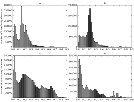
In a first, preprocessing step we evaluate how well our distance metric captures known similarities and differences between protein structures by computing intra-family and inter-family distances. A good distance for structure comparison should pool similar structures, i.e., from the same family, whereas it should locate dissimilar structures from different families far apart from each other. In order to quantify such characteristics, we compute for each family with at least two members a central, representative structure according to Equation (4). Therefore, we compute the distance between any two structures that belong to the same family. Such intra-family distances should ideally be small. We observe that the distribution of intra-family distances differ between classes and are usually smaller than 0.5, except for class c. For the four major protein classes, there is a distance peak close to 0 and another one around 0.2. For the four major protein classes, they are visualized in Figure 3.
Algorithm 1 Solving k-NN classification problem
1: q // Query structure.
2: T // Set of target structures.
3: RF ∀F ∈ C // Family representatives, see (4).
4: d(A, RF) ∀A ∈ F for all families F ∈ C // Distance from all family members
to the respective representative.
5: d(q, RF), d(q, RF) ∀F ∈ C // Bounds on the distance from the query to the
family representatives.
6: LB ← {(t, −∞)|t ∈ T } // Priority queue which will hold the targets t in the order of increasing lower bound distance d5(q, t) to the query.
7: UB ← {(t, ∞)|t ∈ T } // Priority queue which will hold the targets t in the order of increasing upper bound distance d4(q, t) to the query. 8: tUBk // A pointer to the k-th element in UB
9: τ ← 1s // Time limit for pairwise alignment. 10: for F ∈ C do
11: FAM[F ] ← |{t ∈ T : t belongs to family F }| // Number of family members. 12: end for
13: while ∃RF: d(q, RF) 6= d(q, RF) and |T | changes do
14: τ ← τ × 2
15: for F ∈ C with FAM[F ] > 0 do
16: Recompute d(q, RF) and d(q, RF) using time limit τ
17: for t ∈ F do
18: Update priority of t in LB to d5(q, t) = |d(q, RF)−d(RF, t)| // Bound from
inverse triangle inequality (5).
19: Update priority of t in UB to d4(q, t) = d(q, RF) + d(RF, t). // Bound from
triangle inequality (5).
20: end for
21: // Check for targets dominated by tUB
k . 22: for target t in T do 23: if d5(q, t) > d4(q, tUBk ) then 24: T ← T \ t 25: LB ← LB\t 26: UB ← UB\t
27: FAM[F ] ← FAM[F ] − 1 where F the family of t.
28: end if
29: end for
30: end for
31: if |T | = k then
32: return The majority superfamily membership S among T .
33: end if
34: end while
0.0 0.1 0.2 0.3 0.4 0.5 0.6 0.7 0.8 0.9 0 50000 100000 150000 200000 250000 300000 350000 400000
number of inter-family distances
a 0.0 0.1 0.2 0.3 0.4 0.5 0.6 0.7 0.8 0.9 0 500000 1000000 1500000 2000000 b 0.0 0.1 0.2 0.3 0.4 0.5 0.6 0.7 0.8 0.9 0 20000 40000 60000 80000 100000 120000 140000 160000 180000
number of inter-family distances
c 0.0 0.1 0.2 0.3 0.4 0.5 0.6 0.7 0.8 0.9 0 50000 100000 150000 200000 250000 300000 350000 d
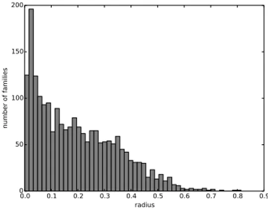
We then compute a radius around the representative structure that encompasses all structures of the corresponding family. The number of families with a given radius decreases nearly linearly from 0 to 0.6, with most families having a radius close to zero, and almost no families having a radius greater 0.6. The histogram of family radii is visualized in Figure 4.
0.0 0.1 0.2 0.3 0.4 0.5 0.6 0.7 0.8 0.9 radius 0 50 100 150 200 number of families
Fig. 4. A histogram of the radii of the multi-member families.
Considering that the distance metric is bound to be within 0 and 1, inter-family distances and radii show that the distance overall captures well the similarity between structures. Further, we investigate the distance between protein families by computing their overlap value as defined by d(rF1, rF2) −
rF1 − rF2. Most families are not close to each other according to our distance
metric. Families of the four most populated classes which belong to different superfamilies overlap in 23-25% of cases for class a, 11-18% for class b, 10-22% for class c and 11-18% for class d. These bounds on the number of overlapping families can be obtained by using the lower and upper bounds on the distances between representatives and the distances between family members appropriately.
5.2 Results for SCOPCath benchmark
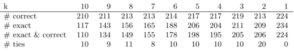
When classifying the 236 queries of SCOPCath, we achieve between 89 and 95% correct superfamily assignments, see Table 3. Remarkably, the highest accuracy is reached for k=1, so here just classifying the query as belonging to the superfamily of the nearest neighbor is the best choice. Our k-NN classification resulted for any k in a large number of ties, especially for k=2, see Table 3. These currently unresolved ties also decrease assignment accuracy compared to k = 1, for which a tie is not possible. Table 3 further lists the number of queries which have been assigned, where exact denotes that the provable k nearest neighbors have
been computed. The percentage of exactly computed nearest neighbors varies between 50 and 99 % and increases with decreasing k. A likely reason for this is that the larger k, the weaker is the k-th distance upper bound that is used for domination, especially if the target on rank k is dissimilar to the query. Since SCOPCath domains have low sequence similarity, this is likely to happen. It is also interesting to note that there are for any k quite a few queries which have been assigned exact, but which are nonetheless wrongly assigned, see Table 3. These are cases in which our distance metric fails in ranking the targets correctly with respect to gold standard.
Table 2. Classification results showing the number of queries out of overall 236 queries that have been assigned to a superfamily, the number of correct assignments, the number of assignments computed exactly, thereof the number of correct classifications and the number of ties which do not allow a family assignment based on majority vote.
k 10 9 8 7 6 5 4 3 2 1
# correct 210 211 213 213 214 217 217 219 213 224
# exact 117 143 156 165 188 206 204 211 209 234
# exact & correct 110 134 149 155 178 198 195 205 206 224
# ties 10 9 11 8 10 10 10 10 20 0
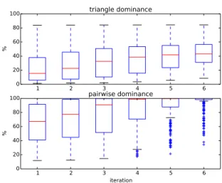
Figure 5 displays the progress of our algorithm in terms of percentages of removed targets. We initially compute six rounds of triangle dominance, starting with 1 CPU s for every query representative alignment and doubling the run time every iteration up to 32 CPU s. The same is done in the pairwise dominance step of the algorithm, in which we compute the distance from the query to every remaining target. As shown in Figure 5, the percentage of dominated targets within each iteration varies widely between queries, which results in a large variance of run times between queries. For some queries, up to 80% of targets can be removed by just computing the distance to the family representatives using a time limit of 1s and applying triangle dominance, for others, even after several iterations of pairwise dominance, 50% of targets remain. Overall, most queries need, after triangle dominance, several iterations of pairwise dominance before being assigned and quite a few even cannot be assigned exactly.
5.3 Results for extended SCOPCath benchmark
Our exact k-NN classification can also be successfully applied to larger benchmarks like extended SCOPCath, which are more representative of databases such as SCOP. Here, the benefit of using a metric distance, triangle inequality and k-NN classification is more pronounced. Remarkably, our classification run time on this benchmark that is about an order of magnitude larger than SCOPCath is for most queries of the same order of magnitude as run times on SCOPCath (except for some queries which need an extremely long
1 2 3 4 5 6 0 20 40 60 80 100 % triangle dominance 1 2 3 4 5 6 iteration 0 20 40 60 80 100 % pairwise dominance
Fig. 5. Boxplots of the percentage of removed targets at each iteration during triangle and pairwise dominance for the 236 queries of the SCOPCath benchmark.
run time and finally cannot be assigned exactly). Also here, run time varies extremely between queries, between 0.15 and 85.63 hours for queries of the four major classes which could be assigned exactly. The median run time for all 1120 exactly assigned extended SCOPCath queries is 3.8 hours. The classification results for extended SCOPCath are shown in Table 3. Slightly more queries have been assigned correctly compared to SCOPCath and significantly more queries have been assigned exactly. Both may reflect that there are now more similar structures within the targets. Further, the number of ties is decreased. Figure 6
Table 3. Classification results showing the number of queries out of overall 1369 queries that have been assigned to a superfamily, the number of correct assignments, the number of assignments computed exactly, thereof the number of correct classifications and the number of ties which do not allow a family assignment based on majority vote.
k 10 9 8 7 6 5 4 3 2 1
# correct 1303 1331 1334 1341 1341 1346 1344 1351 1348 1361
# exact 1120 1182 1228 1271 1286 1339 1341 1352 1347 1368
# exact & correct 1104 1166 1215 1257 1276 1329 1330 1341 1343 1360
# ties 35 5 12 6 11 7 9 3 17 0
displays the progress of the computation. Here, many more target structures are removed by triangle dominance and within the very first iteration of pairwise dominance compared with the SCOPCath benchmark. For example, for most queries, more than 70% of targets are removed by triangle dominance alone. Only
very few queries need to explicitly compute the distance to a large percentage of the targets, and almost 75% of queries can be assigned after only one round of pairwise dominance. 1 2 3 4 5 6 0 20 40 60 80 100 % triangle dominance 1 2 3 4 5 6 iteration 0 20 40 60 80 100 % pairwise dominance
Fig. 6. Boxplots of the percentage of removed targets at each iteration during triangle and pairwise dominance for the 1369 queries of the extended SCOPCath benchmark.
6
Discussion
The difficulty to optimally compute a superfamily assignment using k-NN increases with the dissimilarity of the k-th closest target and the query, because this target determines the domination bound. This can be observed in the different number of exactly assigned queries between SCOPCath and extended SCOPCath on the one side and for different k on the other side. Since SCOPcath has been filtered for low sequence identity, we can expect that the k-th neighbor is less similar to the query than the k-th neighbor in extended SCOPCath, and therefore, it is easier to compute extended SCOPCath exactly. Accordingly, the number of exactly assigned queries tends to increase with decreasing k. In future work, we may use such properties of the distance bounds to decide which k is most appropriate for a given query.
Our exact classification is based on a well-known property of exact CMO computation: similar structures are quick to align, and usually computed exactly, whereas dissimilar structures are extremely slow to align and usually not exactly. Therefore, we remove dissimilar structure early using bounds. Similar structures can then be computed (near-)optimal and the resulting k-NN classification is exact.
Although current results suggest that in terms of assignment accuracy, using only the nearest neighbor for classification works best, finding the k nearest neighbor structures is still interesting and important. A new query structure is in need of being characterized, and a set of k closest structures from a given classification gives a good impression on its location in structure space, especially if this space is metric. Note that, besides using the presented algorithm for determining the k nearest neighbors, it could straightforwardly also be used to find all structures within a certain distance threshold of a given query.
We show that our approach is beneficial for handling large data sets whose structures form clusters in some metric space because it can quickly discard dissimilar structures using metric properties such as triangle inequality. This way, the target data set does not need to be reduced previously using a different distance measure such as sequence similarity, which can lead to mistakes. Our classification is at all times only based on structural distance.
The disadvantage of heuristics for the task of large-scale structure classifica-tion is that these classificaclassifica-tions are not stable. As versions of tools or random seeds change, the distance between structures may change, since the provable distance between two structures is not known. With these distance changes, also the entire classification may change. Such possible, unpredictable changes in classification contradict the essential use of an automatic classification as a reference.
7
Conclusion
In this work we introduced a new distance based on the CMO measure and proved that it is a true metric, which we call the max-CMO metric. We analyzed the potential of max-CMO for solving the k-NN problem efficiently and exactly and built on that basis a protein family classification algorithm. Depending on the values of k, our accuracy varies between 89 % for k = 10 and 95 % for k = 1 for the SCOPCath benchmark. The fact that the accuracy is highest for k = 1 indicates that using more sophisticated rule than k-NN may produce even better results. We also leave a thorough comparison to classification algorithms based on different concepts for further work.
In summary, our approach provides a general solution to k-NN classification based on a computationally intractable metric for which upper and lower bounds are available that can successfully be applied for exact large-scale protein superfamily classification.
References
1. N. S. Altman. An introduction to kernel and nearest-neighbor nonparametric regression. The American Statistician, 1992.
2. R. Andonov, N. Malod-Dognin, and N. Yanev. Maximum contact map overlap revisited. J Comput Biol, 18(1):27–41, 2011.
3. F. Bernstein, T. Koetzle, G. Williams, E. M. Jr., M. Brice, J. Rodgers, O. Kennard, T. Shimanouchi, and M. Tasumi. The protein data bank: A computer-based archival file for macromolecular structures. J. of Mol. Biol., 112:535, 1977. 4. A. Caprara, R. Carr, S. Istrail, G. Lancia, and B. Walenz. 1001 optimal PDB
structure alignments: integer programming methods for finding the maximum contact map overlap. J Comput Biol, 11(1):27–52, 2004.
5. K. L. Clarkson. Nearest-neighbor searching and metric space dimensions. In Nearest-Neighbor Methods for Learning and Vision: Theory and Practice. MIT Press, 2006.
6. G. Csaba, F. Birzele, and R. Zimmer. Systematic comparison of SCOP and CATH: a new gold standard for protein structure analysis. BMC Struct Biol, 9:23–23, 2009. 7. A. Godzik, J. Skolnick, and A. Kolinski. Regularities in interaction patterns of
globular proteins. Protein Eng, 6(8):801–810, 1993.
8. D. Goldman, S. Istrail, and C. Papadimitriou. Algorithmic aspects of protein structure similarity. Foundations of Computer Science, 1999. 40th Annual Symposium on, pages 512–521, 1999.
9. T. Harder, M. Borg, W. Boomsma, P. Røgen, and T. Hamelryck. Fast large-scale clustering of protein structures using Gauss integrals. Bioinformatics, 28(4):510– 515, 2012.
10. N. Malod-Dognin, R. Andonov, and N. Yanev. Maximum cliques in protein structure comparison. In Experimental Algorithms, volume 6049 of Lecture Notes in Computer Science, pages 106–117. Springer, Berlin, Heidelberg, 2010.
11. N. Malod-Dognin, M. L. Boudic-Jamin, P. Kamath, and R. Andonov. Using dominances for solving the protein family identification problem. In T. Przytycka and M.-F. Sagot, editors, Algorithms in Bioinformatics, volume 6833 of Lecture Notes in Computer Science, pages 201–212. Springer Berlin Heidelberg, 2011. 12. N. Malod-Dognin and N. Przulj. Gr-align: fast and flexible alignment of protein
3d structures using graphlet degree similarity. Bioinformatics, 2014.
13. M. L. Mico, J. Oncina, and E. Vidal. A new version of the nearest-neighbour approximating and eliminating search algorithm (aesa) with linear preprocessing time and memory requirements. Pattern Recognition Letters, 15:9–17, 1994. 14. F. Moreno-Seco, L. Mico, and J. Oncina. A modification of the laesa algorithm for
approximated k-nn classification. Pattern Recognition Letters, 24:47–53, 2003. 15. A. G. Murzin, S. E. Brenner, T. Hubbard, and C. Chothia. SCOP: a structural
classification of proteins database for the investigation of sequences and structures. J Mol Biol, 247(4):536–540, 1995.
16. C. A. Orengo, A. D. Michie, S. Jones, D. T. Jones, M. B. Swindells, and J. M. Thornton. CATH–a hierarchic classification of protein domain structures. Structure, 5(8):1093–1108, 1997.
17. D. A. Pelta, J. R. Gonz´alez, and M. Moreno Vega. A simple and fast heuristic for protein structure comparison. BMC Bioinformatics, 9:161–161, 2008.
18. P. Rogen and B. Fain. Automatic classification of protein structure by using gauss integrals. Proceedings of the National Academy of Sciences of the United States of America, 100(1):119–124, 2003.
19. I. Wohlers, N. Malod-Dognin, R. Andonov, and G. W. Klau. CSA: comprehensive comparison of pairwise protein structure alignments. Nucleic Acids Research, 40(W1):W303–W309, 2012.
20. W. Xie and N. V. Sahinidis. A reduction-based exact algorithm for the contact map overlap problem. J Comput Biol, 14(5):637–654, 2007.