HAL Id: hal-01792676
https://hal.archives-ouvertes.fr/hal-01792676
Submitted on 15 May 2018
HAL is a multi-disciplinary open access
archive for the deposit and dissemination of
sci-entific research documents, whether they are
pub-lished or not. The documents may come from
teaching and research institutions in France or
abroad, or from public or private research centers.
L’archive ouverte pluridisciplinaire HAL, est
destinée au dépôt et à la diffusion de documents
scientifiques de niveau recherche, publiés ou non,
émanant des établissements d’enseignement et de
recherche français ou étrangers, des laboratoires
publics ou privés.
Existence of Moffatt vortices at a moving contact line
between two fluids
Mijail Febres Soria, Dominique Legendre
To cite this version:
Mijail Febres Soria, Dominique Legendre. Existence of Moffatt vortices at a moving contact line
between two fluids. Physical Review Fluids, American Physical Society, 2017, vol. 2 (n° 11), pp.
114002/1-114002/2. �10.1103/PhysRevFluids.2.114002�. �hal-01792676�
Open Archive TOULOUSE Archive Ouverte (OATAO)
OATAO is an open access repository that collects the work of Toulouse researchers and
makes it freely available over the web where possible.
This is an author-deposited version published in:
http://oatao.univ-toulouse.fr/
Eprints ID: 19937
To link to this article: DOI: 10.1103/PhysRevFluids.2.114002
URL:
http://dx.doi.org/10.1103/PhysRevFluids.2.114002
To cite this version : Febres Soria, Mijail and Legendre, Dominique
Existence of Moffatt vortices at a moving contact line between two
fluids. (2017) Physical Review Fluids, vol. 2 (n° 11). pp.
114002/1-114002/2. ISSN 2469-990X
Any correspondence concerning this service should be sent to the repository
administrator:
[email protected]
PHYSICAL REVIEW FLUIDS 2, 114002 (2017)
Existence of Moffatt vortices at a moving contact line between two fluids
Mijail Febres and Dominique Legendre*Institut de Mécanique des Fluides de Toulouse, IMFT, Université de Toulouse, CNRS-Toulouse, France
(Received 2 June 2017; published 27 November 2017)
According to Kirkinis and Davis [J. Fluid Mech. 746,R3(2014)], the motion of a contact line can produce a sequence of moving eddies, commonly known as Moffatt vortices. In this work, we extend the formulation given in Kirkinis and Davis for the moving contact line between two viscous fluids and a nonzero static contact angle, and we consider the flow structure in the corner between the interface and the wall. In particular, we discuss the condition for observing Moffatt vortices and we demonstrate that an infinite series of Moffatt vortices cannot be observed considering a Navier-slip boundary condition. DOI:10.1103/PhysRevFluids.2.114002
I. INTRODUCTION
Nonconventional Stokes flow in corners formed by combinations of rigid and free surfaces was first studied theoretically by Moffatt [1]. In that work, the flow in the corner was due to the motion of the fluid far from it, giving rise to a sequence of eddies known as Moffatt vortices. This subject has been addressed since then for many configurations, i.e., Davis and O’Neill [2], Anderson and Davis [3], and, more recently, Malhotra et al. [4], Escudier et al. [5], Scoot [6], and Shtern [7]. The works of Anderson and Davis [3] and Shtern [7] have already shown the presence of Moffatt vortices on the corner formed by a rigid and a two-fluid static free surface, although they considered the no-slip boundary condition on the solid surface. On the other hand, Kirkinis and Davis [8], using a novel slippage model [9], demonstrated the existence of such vortices for a perfectly wetting liquid (αs=0) in the vicinity of a moving contact line using Navier-slip law with a slip length of the form λ = ℓn/rn−1−b(α,n)r, where ℓ is a macroscopic scale, b(α,n) is a dimensionless quantity determined by the boundary conditions, n is a complex number part of the stream function solution, and α is the dynamic angle made by the interface and the wall. Neglecting the outer fluid influence and considering a static contact angle αs=0, the unbalanced Young stress is used to provide a relation between n, b, and the capillary number Ca = µU/γ where U , µ, and γ are the contact line speed, the dynamic viscosity of the advancing fluid, and the surface tension, respectively. Here, we derive a partial local solution based on the slip description given in Kirkinis and Davis [9] in order to consider the flow structure in the corner made by the moving contact line. Given that Moffatt vortices in the corner made between a moving contact line and a wall have not been observed so far in experiments, we discuss their existence on both sides of the interface and the physical relevance of the slip law proposed in Kirkinis and Davis [9]. The work is organized as follows. We derive the local partial solution in Sec.IIand the reader is referred to the Appendices to find more details on the derivation. SectionIIIis dedicated to describe the flow structure as a function of the parameters considered in this work. In Sec.IVwe analyze and discuss the results and their implications.
II. LOCAL ANALYSIS
We consider a moving contact line formed by two viscous fluids and a horizontal solid surface (see Fig. 1). The contact line velocity is U and the angle made by the advancing fluid is α. A “partial local analysis” can be conducted considering that the flow matches with the outer flow at a large distance from the corner [1] (typically, the bulk recirculation for a sliding drop). Partial
*Corresponding author: [email protected]
φ= α Fluid 1 Fluid 2 U r φ
FIG. 1. Schematic representation of a moving contact line between the advancing fluid (k = 1) and the receding fluid (k = 2) (the interface between the two fluids is shown in red) in the reference frame attached to it for a positive value of the contact line speed U in a polar system of coordinates.
local solutions describe situations in which all the local boundary conditions are satisfied with the exception of the normal-stress condition [3]. In practice, this assumption is valid for an interface in the limit of zero capillary number.
In the reference frame of the moving contact line, the Stokes approximation is valid as we approach its origin (r → 0). Also, if radial and azimuthal components (uk, vk) of velocity are expressed in terms of the stream function ψkfor fluid k (k = 1 is for the advancing fluid and k = 2 for the displaced one), Stokes equations yield the biharmonic equation
∇4ψk=0, (1)
which has separable solutions of the form
ψk =rn+1fk(n,φ), (2)
where the function fkhas the form:
fk(n,φ) = Akcos[(n + 1)φ] + Bksin[(n + 1)φ] + Ckcos[(n − 1)φ] + Dksin[(n − 1)φ]. (3) In general, n can be a complex number n = nR+inI and the real part of ψk is then considered [1,6]. In expression (3), Ak, Bk, Ck, and Dk are constants obtained from the following boundary conditions:
(i) At φ = 0, Navier slip and vanishing azimuthal component of velocity u1−U =
λ1 r
∂u1
∂φ; v1=0. (4)
(ii) At φ = π , Navier slip and vanishing azimuthal component of velocity u2+U = −
λ2 r
∂u2
∂φ; v2=0. (5)
(iii) At φ = α, continuity of radial velocity, vanishing azimuthal component of velocity, and balance of shear stress
u1=u2; v1=v2=0; τ1 =τ2. (6)
Following Kirkinis and Davis [8], the slip model proposed by Kirkinis and Davis [9] is considered here in both fluids:
λk =ℓn/rn−1−bk(α,n) r for r 6 rk∗, (7)
EXISTENCE OF MOFFATT VORTICES AT A MOVING . . .
(b) (a)
FIG. 2. Stream function for α = 1 rad, Ca = 0.01, Ŵ = 1 × 10⁻⁶. (a) Solution obtained following Kirkinis
and Davis [8]: n = 6.999193 + 1.278230i, (b) our corrected derivation: n = 6.799117 + 1.648136i. By definition, this slip length vanishes at r = rk∗ =ℓ/b
1/n
k if n is a real number (nI =0). Considering a characteristic velocity U ∼ 1 mm/s, Kirkinis and Davis [9] reported r∗∼0.68 mm for glycerine, and r∗ ∼1 µm for water. Note that when n is a complex number (n
I 6=0), it follows that both quantities λkand ℓ/b
1/n
k are complex numbers.
The combination of the boundary conditions for the velocity at φ = 0 and π and for the azimuthal velocity at the interface makes possible the expressions of constants Ak, Bk, Ck, and Dkas a function of n, bk, and α (see AppendixA). The value of n and bkare then determined by solving the system of equations formed with the tangential conditions at the interface:
f1′−f2′=0; f1′′−Ŵf2′′=0, (9)
and with the noncompensated Young force (see AppendixB) cos αs−cos α =
Ca n
¡
Ŵr2∗n+r1∗n¢, (10)
where Ca = µ1U/γ is the capillary number based on the viscosity of the advancing fluid and Ŵ = µ2/µ1 the viscosity ratio. A value of Ŵ → 0 indicates that a fluid is pushing another fluid of much smaller viscosity (typically a drop spreading in a gas) while the opposite limit, Ŵ → ∞, corresponds to a fluid pushing another fluid of much larger viscosity (for example, a bubble spreading in a liquid). Note that in Kirkinis and Davis [8], the radial position r∗
1 (a real number) has been replaced by ℓ/b11/nin Eq. (10) which is not correct because if n is complex then it follows that ℓ/b1/n is complex. The effect of this correction is shown in Fig.2.
Figure 2reports the streamlines in the limit Ŵ → 0, for αs =0 and α = 1 rad corresponding to the case reported in Kirkinis and Davis [8]. The solution shown in Fig.2(a)is obtained with the derivation proposed by Kirkinis and Davis [8] while the streamlines shown in Fig. 2(b) are obtained with our corrected solution. Following the Kirkinis and Davis [8] derivation, we obtain n =6.999190 + 1.278228i in perfect agreement with their solution. Note that considering Ŵ = 1 × 10⁻⁶instead of Ŵ = 0 [this is the case shown in Fig.2(a)] gives the same streamlines and a very close value for n, n = 6.999193 + 1.278230i. Despite noticeable changes in the streamlines shape, the flow structure in the receding fluid (not considered in Kirkinis and Davis [8]) also reveals the development of Moffatt vortices of similar shape on both sides of the interface.
III. RESULTS
Equation (9) is solved numerically using “fsolve” inside MATLAB which uses the Levenberg-Marquardt and trust-region-reflective methods [10] with default parameters. We can select the solu-tion with the smallest positive nRbecause it determines the asymptotic flow pattern at leading order [7], but the solution may also be imposed by the flow far from the contact line [8]. Multiple solutions for n can be obtained for each set of parameters (Ŵ, α, αs, Ca) that can be varied independently. The flow structure is significantly changed depending if n is a real or a complex number.
0 60 120 180 α 0 5 10 nR (a) 0 60 120 180 α 0 5 10 nR (b) 0 60 120 180 α 0 5 10 nR (c) 0 60 120 180 α 0 5 10 nR (d) 0 60 120 180 α 0 5 10 nR (e) 0 60 120 180 α 0 5 10 nR (f)
FIG. 3. Map of real solutions for Ca = 0.01 and (a) Ŵ = 0.01, (b) Ŵ = 0.1, (c) Ŵ = 1, (d) Ŵ = 2, (e) Ŵ =10, (f) Ŵ = 100.
A. Regular corner flows (real solutions for n)
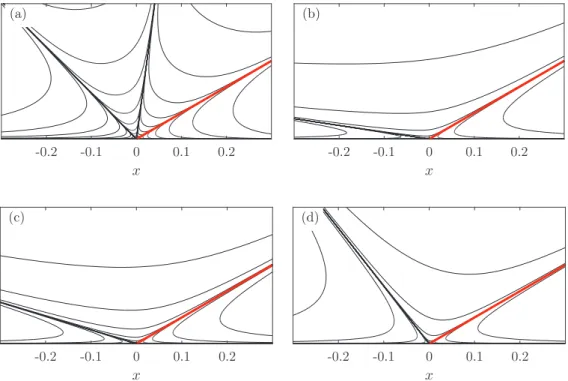
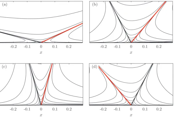
The solution with real values for n are reported in Fig.3as a function of α for Ca = 0.01 and for viscosity ratio from Ŵ = 0.01 to 100 in order to cover both gas-liquid and liquid-liquid interfaces. Both the density of solutions and the appropriate angle for having a solution are clearly depending on α and Ŵ. It seems that available solutions can be found for any angle. The density of the solution increases with Ŵ. Note that the map of solutions is different between large and small Ŵ. Indeed, Ŵ and 1/ Ŵ do not play a symmetrical role in Eq. (10). Below the threshold nR =1, shown using a dotted red line, no valid description of the shear and pressure can be obtained as r → 0, as it is in the case of the no-slip boundary condition, because shear and pressure are both varying as rn−1. Streamlines are shown in Figs.4and in5where different values of Ŵ and α are considered, respectively. The flow behaves like a classical flow in a corner. The main feature of the flow structure is that it can be split depending on the conditions. For example, in Fig.4where the effect of Ŵ is reported for the imposed dynamic contact angle α = 30◦, the flow only splits in fluid 2 while the flow can also be split in the two fluids as shown in Fig.5(b). Huh and Scriven [11] observed, with a no-slip boundary conditions for the two fluids, that there is a tendency of this splitting to appear in the fluid with the lower viscosity, while here we observe the opposite attributed to the imposed slip condition. We have also to mention that larger numbers of flow splitting appear with the increase of n. This is, for example, the case in Fig.4(a)where two splits are present in fluid 2.
B. Moffatt vortices (complex solutions for n)
Moffatt vortices are observed for complex solution for n. Because of the continuity of the velocity at the interface, each vortex in the advancing fluid is connected at the interface to its counterpart in the receding fluid 2, so that a pair of vortices can be identified and infinite series of Moffatt vortices are observed on both sides of the interface. In the following, we call vortices 1 and 2 the vortices in the advancing fluid 1 and in the receding fluid 2, respectively.
EXISTENCE OF MOFFATT VORTICES AT A MOVING . . . (a) -0.2 -0.1 0 0.1 0.2 x (b) -0.2 -0.1 0 0.1 0.2 x (c) -0.2 -0.1 0 0.1 0.2 x (d) -0.2 -0.1 0 0.1 0.2 x
FIG. 4. Effect of Ŵ. Stream function for α = 30◦, α
s =0◦, and Ca = 0.01. (a) Ŵ = 0.1, n = 3.490212;
(b) Ŵ = 1, n = 1.253249; (c) Ŵ = 2, n = 1.202459; (d) Ŵ = 10, n = 1.246048.
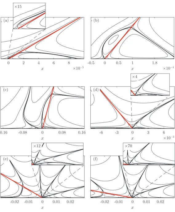
Examples of streamlines are reported in Figs.6and in7where the effect of the dynamic contact angle and the viscosity ratio are shown, respectively. Comparing the streamlines in these figures, it is clear that their shapes are very sensitive to these two parameters. Different types of Moffatt vortices can be identified: the “corner vortex” [see Fig.6(b)in the advancing fluid], the “detached corner vortex” [see Figs.7(c)and7(d)in the receding fluid], the “wall vortex” [see Fig.6(a)in the advancing fluid], and the “interface vortex” [see Fig.6(b)for the receding fluid]. In addition, it is also clear from these figures that the vortex size is different when comparing fluids 1 and 2. For example, in Fig.6(a), a zoom is necessary to visualize the vortex 2 that matches to its corresponding vortex 1 at the interface: vortex 2 is here more than one order of magnitude smaller than vortex 1. The velocity being continuous at the interface, a smaller vortex reveals a vortex of stronger vorticity. In Fig. 7, we observe that vortex 1 becomes significantly much smaller than vortex 2 when Ŵ increases. This is consistent with the consideration that the motion is facilitated in the less viscous fluid than in the more viscous fluid. The inspection of the effect of both the capillary number Ca and the static angle αs (not shown here) reveals that the fluid structure is preserved when varying independently these two parameters. In fact, considering the system of Eqs. (9) and (10), Ca and αs are both impacting the solution by relation (10) so that the relevant parameter to consider is f
Ca = Ca/(cos αs−cos α) which measures the ratio of viscous force to the noncompensated Young force. The cases for α = 90◦, Ŵ = 1, and α
s =0 (not shown here) are characterized by a perfect symmetry of the solution with respect to the interface.
IV. DISCUSSION
Moffatt vortices are observed for solutions where n is a complex number. As a consequence, the slip length as proposed by Kirkinis and Davis [8] [see Eq. (7)] used in the derivation is then a complex number. The solution of interest being given by the real part of the stream function, the slip length, as defined by Eq. (7) is not the effective slip experienced by the two fluids at the wall.
(a) -0.2 -0.1 0 0.1 0.2 x (b) -0.2 -0.1 0 0.1 0.2 x (c) -0.2 -0.1 0 0.1 0.2 x (d) -0.2 -0.1 0 0.1 0.2 x
FIG. 5. Effect of α. Stream function for Ca = 0.01, Ŵ = 1, and αs=0. (a) α = 25◦, n = 1.272566;
(b) α = 50◦, n = 3.556807; (c) α = 75◦, n = 2.613791; (d) α = 130◦, n = 3.560146.
The normalized effective slips at the wall for the advancing and receding fluids, λ1Eand λ2E, are to be deduced from the real part of the solution for φ = 0 and π , respectively, as (the normalization is based on U and ℓ as introduced in AppendixA)
R(u1−1) = λ1ER µ 1 r ∂u1 ∂φ ¶ ; R(u2+1) = λ2ER µ −1 r ∂u2 ∂φ ¶ . (11)
Here, R(z) and I (z) stand for the real and the imaginary parts of the complex number z. Considering the advancing fluid (k = 1), the radial velocity at the wall is
R[u1(φ = 0)] = rnR{cos[nIln(r)]R(f1′|φ=0) − sin[nIln(r)]I (f1′|φ=0)}, (12) while the velocity gradient at the wall is
R Ã 1 r ∂u1 ∂φ ¯ ¯ ¯ ¯ φ=0 ! =rnR−1{cos[n Iln(r)]R(f1′′|φ=0) − sin[nIln(r)]I (f1′′|φ=0)}. (13)
From the boundary conditions at φ = 0, we get f1′|φ=0=b1, f ′′
1|φ=0= −1, and the effective slip length experienced by the fluid on the wall is then
λ1E= −rR(b1) + r tan[nIln(r)]I (b1) +
1
rnR−1cos[nIln(r)]. (14)
Note that the value of the radial position on the wall r = r∗
1 where the slip length cancel [and used in Eq. (10)] comes from this relation. Following the same derivation for the receding fluid we can show that for both fluids rk∗is given by
EXISTENCE OF MOFFATT VORTICES AT A MOVING . . . (a) 0 2 4 6 8 x ×10−5 ×15 (b) -0.5 0 0.5 1 1.8 x ×10−4 (c) -0.16 -0.08 0 0.08 0.16 x (d) -6 -3 0 3 6 x ×10−3 ×4 (e) -0.02 -0.01 0 0.01 0.02 x ×12 (f) -0.02 -0.01 0 0.01 0.02 x ×70
FIG. 6. Effect of α. Stream function for Ca = 0.01, Ŵ = 0.1, and αs =0. (a) α = 30◦ (n = 2.049237 +
0.242136 i); (b) α = 50◦ (n = 2.231697 + 0.319340 i); (c) α = 75◦ (n = 2.849756 + 1.033444 i); (d) α =
130◦(n = 2.679453 + 0.383081 i); (e) α = 150◦(n = 4.733359 + 0.381333 i); (f) α = 170◦(n = 4.053887 +
0.403130 i).
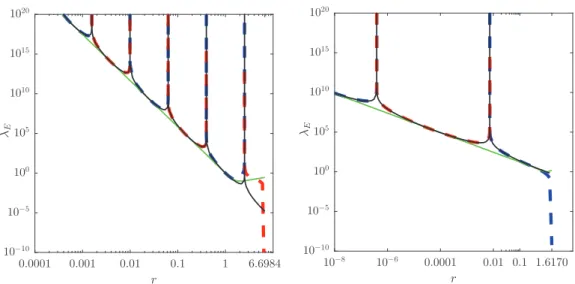
The evolution of the normalized effective slip λ1Ewith r is shown in Fig.8for two cases: the case reported in Kirkinis and Davis [8] [see Fig.2(b)] with n = 6.799117 + 1.648136i (α = 1 rad, Ca = 0.01, Ŵ = 0) and the case shown in Fig. 6(b) with n = 2.231697 + 0.319340 i (α = 50◦, Ca = 0.01, Ŵ = 0.1). The slip length evolution is plotted here up to r = r∗given by Eq. (15) when it cancels. For clarity, the absolute value of λ1E is reported with the use of a log/log scale, red lines are showing negative values of the slip, while blue lines are showing positive values. For both
(a) -0.15 0 0.2 0.4 x (b) -5 0 5 10 18 x ×10−5 (c) -0.06 -0.03 0 0.03 0.06 x ×1000 (d) -6 -3 0 3 6 x ×10−3 ×40 (e) -2 -1 0 1 2 x ×10−5 ×4500 (f) -0.9 -0.4 0 0.4 0.9 x ×10−5 ×150
FIG. 7. Effect of the viscosity ratio Ŵ. Stream function for α = 60◦, Ca = 0.01. (a) Ŵ = 0.01
(n = 2.587148 + 0.349960 i); (b) Ŵ = 0.1 (n = 2.620577 + 0.334090 i); (c) Ŵ = 0.25 (n = 2.675627 + 0.265560 i); (d) Ŵ = 0.8 (n = 2.834106 + 0.400948 i); (e) Ŵ = 1 (n = 2.773461 + 0.210823 i); (f) Ŵ = 2 (n = 2.633405 + 0.209562 i).
cases, the effective slip clearly follows the general trend of the modulus of the “complex” slip λ1 shown in green but we observe periodical changes in the sign of the effective slip length λ1E. In the limit of small r with nR >1, the third term in Eq. (14) is dominant, and Eq. (14) simplifies to λ1E≈1/rnR−1cos [nIln(r)]. This expression is reported using a black line in Fig.8. It clearly shows that it provides a very good description of the evolution of the effective slip with r and it reproduces the successive changes of sign. The normalized wave length 3 for the change of sign can be deduced from this relation as 3 ≈ exp(π/nI) and its magnitude is thus very sensitive to the value of the complex part nI of the solution n. The sign of the effective slip is clearly understood to come from the shear at the wall resulting from the direction of the vortex rotation. A perfect slip
EXISTENCE OF MOFFATT VORTICES AT A MOVING . . . 10−8 10−6 0.0001 0.01 0.1 1.6170 r 10−10 10−5 100 105 1010 1015 1020 λE 0.0001 0.001 0.01 0.1 1 6.6984 r 10−10 10−5 100 105 1010 1015 1020 λE
FIG. 8. Example of effective slip length for the advancing fluid. The absolute value |λ1E|is reported to make
possible the use of a log/log scale. The solid red line denotes the negative value of λ1Egiven by Eq. (14); the
solid blue line the positive value of λ1Egiven by Eq. (14); the solid black line λ1E≈ℓ/rnR−1cos [nIln(r/ℓ)];
and the solid green line the modulus of Eq. (14). (Left) For the case reported in Kirkinis and Davis [8] shown in Fig.2(b), n = 6.999190 + 1.278228 i (Ca = 0.01, Ŵ = 0, α = 1 rad). (Right) For the case shown in Fig.6(b), n =2.231697 + 0.319340 i (Ca = 0.01, Ŵ = 0.1, α = 50◦).
(zero shear) is observed between two vortices. It is clear that such a slip behavior is questionable for real surfaces where a positive slip is expected. As shown in Fig.8(b), the slip has a positive value before it cancels while it is negative in Fig.8(a). The case with a positive slip may be consistent with the existence of only one vortex in the corner. Following Moffatt [1], we can show that the ratio ρ of the distance to the corner of two successive vortices is given in each fluid by ρ = exp(π/nI). We recover here the wavelength 3 observed for the change of sign. This relation indicates that small values of nI induce a relative large distance between two successive vortices. An infinite vortex observation being limited in real flows by the continuum limit, in some cases only one vortex may be observed making consistent the proposed slip. Taking for instance a millimetric drop of water moving on a plane surface in a more viscous oil, the selected solution for n has to satisfy nI ∼0.2, corresponding for example to the solution found for α = 60◦, Ca = 0.01, and Ŵ = 2 and reported in Fig.7(f).
We end the discussion by considering a slip length of the general form λk(r) for both the advancing and the receding fluids, with the imposed condition that λk(r) is positive and real. Different slip models have been reported (see, for example, Dussan [12] and Sibley et al. [13]) to consider the singularity of the solution close to the contact line. Imposing a zero-slip condition gets n = 0 and the solution has the form ψ = r(Aφ cos φ + Bφ sin φ + C cos φ + D sin φ) with both stress and pressure diverging [11] as r−1. A constant slip imposes n = 1 and removes the singularity at the contact line in the stress but not in the pressure. The stream function has then the form [3] ψ = r2(A cos 2φ + B sin 2φ + Cφ + D). Nonconstant slip models with n > 1 solve both singularities and the function f has then the shape considered in this work. Replacing the stream function ψk=rn+1fkin relations (4) and (5), we get that the Navier-slip conditions are satisfied if the slip lengths λk(r) have the form
λ1(r) = r f′ 1 ¯ ¯ φ=0 f1′′¯¯φ=0 − 1 rn−1 1 f1′′¯¯φ=0; λ2(r) = − 1 rn−1 1 f2′′¯¯φ=π −r f′ 2 ¯ ¯ φ=π f2′′¯¯φ=π. (16) 114002-9
With relation (16), we can recover the above-mentioned slip lengths and in particular the shape of the slip law introduced by Kirkinis and Davis [9] and considered in our work. As a consequence, this slip law provides the general shape for a Navier-slip length allowing Stokes flow description in a corner. Relation (16) shows that a positive real slip can only be imposed on the wall if n is real, but then the infinite series of Moffatt vortices is not observed. When n is a complex number, then λk(r) is complex and induces a solution with an effective slip as discussed above.
V. CONCLUSIONS
In this work we have reconsidered the derivation proposed in Kirkinis and Davis [8] to study the flow in the corner formed by a moving contact line between two viscous fluids. This extension makes it possible to obtain a complete view of the flow structure for any fluid/fluid and contact angle combination. Solutions for real values of n (the stream function has the form ψk=rn+1fk) provide regular flows in the corner, and flow splitting is observed depending on the parameters. Increasing the values for n increases the number of separations. Solutions for complex values for n result in an infinite series of Moffatt vortices on both sides of the interface. The flow structure is significantly dependent on both the dynamic contact angle and the viscosity ratio while it is weakly affected by the capillary number and the static angle. Moffatt vortices can be located in the center of the wedge (the classical representation of Moffatt vortices), but they can deform and drift to the interface or to the wall. We named these structures as “corner vortices,” “detached corner vortices,” “interface vortices,” and “wall vortices.”
A slip law of the form λ = ℓn/rn−1−b(α,n) r, as proposed by Kirkinis and Davis [9], provides the general shape for a Navier-slip length allowing Stokes flow description in a corner. A positive slip, as observed on real surfaces, can only be imposed on the wall if n is real and then the infinite series of Moffatt vortices cannot be observed. Indeed, a solution with a complex number for n corresponds to an effective slip characterized by alternative changes of sign. However, the cutoff imposed by the continuum limit may restrict the vortex series to only one vortex in the corner. Such a situation with an imposed positive slip may then be selected by the flow. Vortices generated by the motion of a moving contact line have yet to be observed. Well-controlled experiments or direct numerical simulations are required to resolve this point. Note that the presence of internal vortices is connected to a vortex organization in the receding fluid where the vortex detection may be more accessible in experiments.
ACKNOWLEDGMENT
M. Febres gratefully acknowledges financial support from FINCyT under Contract No. 099-FINCyT-BDE-2014.
APPENDIX A: DERIVATION OF THE SOLUTION
The Stokes solution is derived in the polar system of coordinates (r,φ) with the following boundary conditions. The Navier condition and a zero azimuthal velocity on the wall for fluid 1 (φ = 0) and for fluid 2 (φ = π ) are
u1−U = µ ℓn rn−1 −b1r ¶ 1 r ∂u1 ∂φ; v1=0, (A1) u2+U = − µ ℓn rn−1 −b2r ¶ 1 r ∂u2 ∂φ; v2=0. (A2)
The azimuthal velocity, the continuity of both the tangential velocity and the tangential shear writes at the interface (φ = α)
EXISTENCE OF MOFFATT VORTICES AT A MOVING . . .
The system of equations is solved using the stream functions ψk(uk=1r ∂ψk
∂φk and vk= − ∂ψk
∂r):
∇4ψk =0. (A4)
The adimensionalization is performed using U and ℓ, so ˜r = r
ℓ; ψ˜k = ψk
U ℓ. (A5)
Dropping the notation of “tilde” for clarity, the boundary conditions leave at φ = 0 ∂ψ1 ∂r =0; 1 r ∂ψ1 ∂φ −1 = µ 1 rn+1 − b1 r ¶∂2ψ 1 ∂φ2 , (A6) at φ = π ∂ψ2 ∂r =0; 1 r ∂ψ2 ∂φ +1 = µ b2 r − 1 rn+1 ¶ ∂2ψ2 ∂φ2 , (A7) and at φ = α ∂ψ1 ∂r =0; ∂ψ2 ∂r =0; ∂ψ1 ∂φ − ∂ψ2 ∂φ =0; ∂2ψ 1 ∂φ2 −Ŵ ∂2ψ 2 ∂φ2 =0. (A8)
The nondimensional stream functions are expressed as
ψk=rn+1fk, (A9)
where the function fkhas the form
fk(n,φ) = Akcos[(n + 1)φ] + Bksin[(n + 1)φ] + Ckcos[(n − 1)φ] + Dksin[(n − 1)φ], (A10) where Ak, Bk, Ck, and Dkare constants given by the boundary conditions.
Substitution of (A9) into boundary conditions (A6) and (A7) leaves at φ = 0 f1=0; rnf1′−1 = f ′′ 1 −b1rnf1′′, (A11) at φ = π f2=0; rnf2′+1 = r nb 2f2′′−f ′′ 2, (A12) and at φ = α f1=0; f2=0; f1′−f ′ 2=0; f ′′ 1 −Ŵf ′′ 2 =0. (A13)
The slip condition [second condition in (A11) and (A12)] is satisfied in fluid 1 (resp. fluid 2) for any rif f′ 1= −b1f1′′and f ′′ 1 = −1 (resp. f ′ 2 =b2f2′′and f ′′ 2 = −1).
The first eight equations from (A11) to (A13) are used to determine Ak, Bk, Ck, and Dk. We find the following relations for coefficients A1, B1, C1, and D1:
A1= 1
4 n, (A14)
B1=
sin(n α) sin(α) + n (2 b1 sin[α (n − 1)] − sin(n α) sin(α))
4 n sin(n α) cos(α) − 4 n2 cos(n α) sin(α) , (A15) C1= −
1
4 n, (A16)
D1=
sin(n α) sin(α) − n (2 b1 sin[α (n + 1)] − sin(n α) sin(α))
4 n sin(n α) cos(α) − 4 n2 cos(n α) sin(α) , (A17)
and the relations for constants A2, B2, C2, and D2are A2= O W, (A18) B2= Q W, (A19) C2= S W, (A20) D2= −T W , (A21) with
O =sin[α − n (α − 2 π )] − sin[α (n + 1)] + 2 n cos(n α) sin(α) + 2 b2n (cos[α (n − 1)]
−cos[α − n (α − 2 π )]), (A22)
Q =cos[α (n + 1)] − cos[α − n (α − 2 π )] + 2 n sin(n α) sin(α) + 2 b2n (sin[α (n − 1)]
−sin[α − n (α − 2 π )]), (A23)
S =sin[α (n − 1)] + sin[α + n (α − 2 π )] − 2 n cos(n α) sin(α) − 2 b2n (cos[α (n + 1)]
−cos[α + n (α − 2 π )]), (A24)
T =cos[α (n − 1)] − cos[α + n (α − 2 π )] + 2 b2n (sin[α (n + 1)] + sin[α + n (α − 2 π )])
+2 n sin(n α) sin(α), (A25)
W =8 n (sin[n (α − π )] cos(α) − n cos[n (α − π )] sin(α)). (A26) Substitution of these constants into Eq. (A10) provides functions fkand their derivatives as a function of n and bk.
APPENDIX B: NONCOMPENSATED/UNBALANCED YOUNG FORCE
The contact line velocity is expressed here considering the unbalanced Young force following Kirkinis and Davis [9]. The force Fγ that drives this motion is then called “noncompensated Young Force” [14]:
Fγ =γ(cos αs−cos α). (B1)
This force must overcome friction forces caused by the motion of the contact line. The shear stress at the wall, for fluids 1 and 2 (with dimensions), is given by
τ1|φ=0=µ1 1 r2 ∂2ψ 1 ∂φ2 ¯ ¯ ¯ ¯φ=0, (B2) τ2|φ=π =µ2 1 r2 ∂2ψ2 ∂φ2 ¯ ¯ ¯ ¯ φ=π . (B3)
Introducing functions f1and f2for the stream function [Eq. (2) in the paper], τ1|φ=0=µ1 U rn−1 ℓn 1 f1′′¯¯φ=0, (B4) τ2|φ=π =µ2 U rn−1 ℓn1 f ′′ 2 ¯ ¯ φ=π. (B5)
EXISTENCE OF MOFFATT VORTICES AT A MOVING . . .
The total viscous force Fµat the wall exerted by the two fluids is obtained by the integration of the shear in the slip region:
Fµ = Z r∗ 2 0 τ2 ¯ ¯φ=πdr + Z r∗ 1 0 τ1 ¯ ¯φ=0dr. (B6)
Substitution of the shear yields
Fµ= − 1 n ¡
Ŵr2∗n+r1∗n¢. (B7)
The resulting force balance Fγ +Fµ=0 raises to the relation between the dynamic angle, the static angle, and the capillary number:
cos αs−cos α = Ca
n ¡
Ŵr2∗n+r1∗n¢, (B8)
where Ca = µ1U/γ is the capillary number based on the viscosity of the advancing fluid. As discussed in Kirkinis and Davis [9], this relation can be compared to similar relations between the capillary number and the dynamic contact angle [14–16]. The logarithm of the ratio between the macroscopic and molecular length scales that multiplies the capillary number in these relations can be identified here with the exponent n.
[1] H. K. Moffatt, Viscous and resistive eddies near a sharp corner,J. Fluid Mech. 18,1(1964).
[2] A. M. J. Davis and M. E. O’Neill, Separation in a stokes flow past a plane with a cylindrical ridge or trough,Q. J. Mech. Appl. Math. 30,355(1977).
[3] D. M. Anderson and S. H. Davis, Two-fluid viscous flow in a corner,J. Fluid Mech. 257,1(1993). [4] C. P. Malhotra, P. D. Weidman, and A. M. J. Davis, Nested toroidal vortices between concentric cones,
J. Fluid Mech. 522,117(2005).
[5] M. Escudier, J. O’Leary, and R. Poole, Flow produced in a conical container by a rotating endwall,
Int. J. Heat Fluid Flow 28,1418(2007); revised and extended papers from the 5th Conference in Turbulence, Heat and Mass Transfer.
[6] J. F. Scott, Moffatt-type flows in a trihedral cone,J. Fluid Mech. 725,446(2013). [7] V. Shtern, Moffatt eddies at an interface,Theor. Comput. Fluid Dyn. 28,651(2014).
[8] E. Kirkinis and S. H. Davis, Moffatt vortices induced by the motion of a contact line,J. Fluid Mech. 746,
R3(2014).
[9] E. Kirkinis and S. H. Davis, Hydrodynamic Theory of Liquid Slippage on a Solid Substrate Near a Moving Contact Line,Phys. Rev. Lett. 110,234503(2013).
[10] Matlab, matlab version 8.5.0.197613 (R2015a) (The Mathworks, Inc., Natick, Massachusetts, 2015). [11] C. Huh and L. E. Scriven, Hydrodynamic model of steady movement of a solid/liquid/fluid contact line,
J. Colloid Interface Sci. 35,85(1971).
[12] V. E. B. Dussan, The moving contact line: the slip boundary condition,J. Fluid Mech. 77,665(1976). [13] D. N. Sibley, A. Nold, N. Savva, and S. Kalliadasis, A comparison of slip, disjoining pressure, and interface
formation models for contact line motion through asymptotic analysis of thin two-dimensional droplet spreading,J. Eng. Math. 94,19(2015).
[14] F. Brochard-Wyart and P. G. de Gennes, Dynamics of partial wetting,Adv. Colloid Interface Sci. 39,1
(1992).
[15] R. G. Cox, The dynamics of the spreading of liquids on a solid surface, part 1. Viscous flow,J. Fluid Mech. 168,169(1986).
[16] P. G. de Gennes, Wetting: statics and dynamics,Rev. Mod. Phys. 57,827(1985).

![FIG. 2. Stream function for α = 1 rad, Ca = 0.01, Ŵ = 1 × 10 −6 . (a) Solution obtained following Kirkinis and Davis [8]: n = 6.999193 + 1.278230i, (b) our corrected derivation: n = 6.799117 + 1.648136i.](https://thumb-eu.123doks.com/thumbv2/123doknet/14431404.515243/5.892.156.742.200.345/stream-function-solution-obtained-following-kirkinis-corrected-derivation.webp)