1 Introduction
Among a wide range of existing land use change models which are employed to analyse and/or predict future land use patterns, cellular automata (CA) models have been used extensively. CA models address the transitions in space as state changes and simulate the state changes through immediately neighbouring cells (Wu, 2002). Key challenges in CA is calibrating the transition rules of land use change probability from one state to another as a function of (i) the neighbourhood effects and (ii) a series of controlling factors. Logistic regression (logit) has become one of the most popular techniques for calibration of CA models. The logit method can include geophysical as well as socio-economic factors. The model’s ability to include as many socio-economic factors as necessary allows us to better understand human interactions with urban systems. The logit method requires less computation resources for calibration. Despite these strengths, these calibration methods suffer some limitations including autocorrelation. Land use patterns almost show potential spatial autocorrelation caused by a number of centripetal and centrifugal forces which would bias the results of the regression analysis (Overmars et al., 2003). A common approach to minimize the spatial autocorrelation is calibrating the model based on a structured or random sample from the whole dataset, which will lose certain information (Cammerer et al., 2013; Puertas et al., 2014).
With recent advancements in computer and software technologies, researchers have begun to calibrate CA models using a wide range of alternative methods including machine learning (e.g. Rienow and Goetzke, 2015) and optimization techniques such as genetic algorithm (e.g. Al-Ahmadi et al., 2009), particle swarm optimization (e.g. Feng et al., 2011), and Markov Chain Monte Carlo (e.g. Mustafa et al., 2017).
The common optimization algorithms that are introduced in CA models are related to general three categories: (i) evolutionary algorithms, (ii) swarm intelligence algorithms and (iii) stochastic optimization algorithms. A widely used example of the first category is the genetic algorithm (GA) (e.g. Al-Ahmadi et al., 2009; García et al., 2013; Shan et al., 2008; Yang and Li, 2007) whereas the most popular swarm optimization algorithm used in CA urban models is the particle swarm optimization (PSO) (e.g. Feng et al., 2011; Liao et al., 2014; Masoomi et al., 2013). Other optimization algorithms are parallel simulated annealing (PSA) (Al-Ahmadi et al., 2009) which is classified as a stochastic algorithm, and ant colony optimization (Li et al., 2011) which is related to swarm algorithms. Despite the potential of optimization algorithms, only limited efforts have been made to evaluate the performance of such algorithms against each other and against typical CA-logit models. Feng et al. (2011) compared CA-PSO model with CA-logit and argued that the CA-PSO outperformed the CA-logit. Al-Ahmadi et al. (2009) implemented CA-GA and CA-PSA and found that the CA-GA model produced more accurate and consistent results. Previous studies did not analyse the effect of sampling on the performance of different optimization algorithms.
Evaluation of the CA models is another challenge. A common method is based on pixel-by-pixel location agreement. A pixel-by-pixel agreement cannot discriminate between “near-miss” and “far-miss” errors, which limits its ability to detect spatial patterns (Mustafa et al., 2014). Another method is based on fuzzy set theory. Fuzzy map comparison provides a method of dealing and comparing maps containing a complex mixture of spatial information (Ahmed et al., 2013). It measures similarity of a cell in a value between 0 (fully-distinct) and 1 (fully-identical).
This paper applies three optimization algorithms related to three main categories (i) genetic algorithm (GA) as an
Comparison among three automated calibration methods for cellular
automata land use change model: GA, PSO and MCMC
Ahmed Mustafa University of Liège Place du 20 Août 7 Liège, Belgium [email protected] Ismaïl Saadi University of Liège Place du 20 Août 7 Liège, Belgium [email protected] Amr Ebaid Purdue University 305 N University St W Lafayette, IN, USA[email protected] Mario Cools University of Liège Place du 20 Août 7 Liège, Belgium [email protected] Jacques Teller University of Liège Place du 20 Août 7 Liège, Belgium [email protected] Abstract
Spatial cellular automata (CA) model is one of the most common approaches to simulate land use change. Generally, CA estimates the transition likelihood from one land use state to another according to local neighbourhood dynamics and global drivers. Logistic regression (logit) method is widely used to calibrate CA models. Recently, several optimization algorithms have been introduced to calibrate CA models. This study compares the performance of three optimization algorithms: (i) genetic algorithm (GA), (ii) particle swarm optimization (PSO), (iii) and Markov Chain Monte Carlo (MCMC). The three algorithms are incorporated into a CA model to simulate urban expansion in Wallonia (Belgium). In addition, we compare the three calibration algorithms with the logit method. The results show that all three algorithms outperformed the logit method. The results also reveal that the performance of GA is slightly better than PSO and MCMC.
evolutionary algorithm to calibrate CA model, (ii) particle swarm optimization (PSO) as a swarm optimization and (iii) Markov Chain Monte Carlo (MCMC) which is related to stochastic optimization algorithms. The proposed CA model is applied to simulate the urban expansion in Wallonia (Southern Belgium) from 1990 to 2000 as an example application. The model is also calibrated using logit. The simulations of different calibrations under the same conditions are compared with each other to evaluate the performance of each method. The evaluation function is the maximization of accuracy rate for newly urban cells between 1990 and 2000. The evaluation function is defined as a fuzzy membership function of exponential decay with a halving distance of two cells and a neighbourhood window of four cells.
The following sections describe the case study, methodology, results, and then provide conclusions as well as suggestions for future studies.
2 Case Study: Wallonia, Belgium
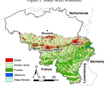
Wallonia is situated in the southern part of Belgium at 49°28' to 50°49' N latitudes and 2°50' to 6°28' E longitudes, Figure 1. Wallonia is the predominantly French-speaking region of Belgium. It accounts for 55% of the territory of Belgium with a total area of 16,844 km². It comprises five provinces: Hainaut, Liège, Luxembourg, Namur, and Walloon Brabant. Wallonia has a pronounced undulating topography. The topography goes from flat to hilly with altitude ranges from 0 to 693 m above see-level. This means cycling is almost non-existent in Wallonia (Dujardin et al., 2012). Major cities in Wallonia are characterized by a strong centre–periphery structure with well-off households located in the peripheries (Verhetsel et al., 2010). Urban sprawl has affected Wallonia for decades leading to fragmented and isolated landscapes that were developed in space and time (Antrop, 2004).
The CORINE Land-Cover (CLC) datasets provide a detailed inventory of the biophysical land cover in Europe using 44 classes. In this case study, the original 44 land-use classes have been reclassified into seven aggregate land-use classes: Urban lands, Arable lands, Grasslands, Forests, Wetlands, Water bodies and Others.
Figure 1: Study Area (Wallonia)
3
CA Model
The model’s space consists of a 2D array of cells of the same dimensions and each time-step represents one year. The quantity of change during model calibration was constrained to the actual quantity of the actual new urban cells between 1990 and 2000 divided evenly by 10 (the number of years). The CA model allocates the required new urban areas based on a probability of a cell (i,j) changing its state from non-urban to non-urban at time t as:
(1)
where
Purb: the urban transition probability of a non-urban cell in a certain time step
Pd: the probability based on a number of urbanization controlling factors
Pn: the neighbourhood effect calculated by using the CA
con: the constraint conditions of land development. con=0
if the original cell state in 1990 is water or urban, otherwise con=1.
In this study, Pn function is calculated as (Feng et al., 2011; Wu, 2002):
∑
(2)
where count(S=urban) is the number of urban cells amongst the Moore n×n neighbourhood. In this study, a 3×3 Moore neighbourhood is used to consider neighbourhood interactions.
Pd represents an urbanization probability map of non-urban lands to convert into urban lands based on a set of urbanization controlling factors as
1111 2222
exp ... 1 exp ... n n n n d X X X X X X P (3)where X1… Xn represent the controlling factors behind urban expansion and α and β1… βn are the model parameters that need to be calibrated. These parameters are calibrated based on four methods: (i) logistic regression, (ii) genetic algorithm, (iii) particle swarm optimization and (iv) Markov Chain Monte Carlo. As stated above, logit suffers from spatial autocorrelation that exists in the model input data. We calibrate the model using random sampling approach. The selection of the appropriate sample is done based on the CA-logit performance with 100 different random samples. The sampling set that produces the best result will be introduced in the final calibration phase of all methods. We also run all calibration methods using all data without considering sampling approach.
Figure 2 illustrates the urbanization controlling factors introduced in this study. All maps were created as raster grids with a resolution of 100×100 meters.
Figure 2: The urbanization controlling factors Distance to Highways Distance to major roads Distance to secondary roads Distance to local roads Distance to cities Employment potential Spatial policy (zoning)
3.1 Logistic Regression
Logit is a popular method for discovering the empirical relationships between a discrete dependent variable and a number of indented variables (controlling factors). In this study, the dependent variable is a binary showing the observed changes from non-urban to urban (coded as 1) and cells whose status remains non-urban (coded as 0).
3.2 Genetic Algorithm
GA is an effective optimization algorithm. It has been inspired by the mechanisms of evolution and genetics. The algorithm generates the initial population (generation) at random. Each individual in this population represents a combination of CA parameters. For each new generation, it randomly selects individuals from the current population to be parents and uses them to produce the children for the next generation using crossover and mutation operators. Both operators drive the population toward an optimal solution over successive generations.
3.3 Particle Swarm Optimization
In a typical particle swarm optimization scenario (PSO), we work with a population (swarm) of candidate solutions (particles). PSO has been inspired by different patterns in artificial life, such as bird flocking and fish schooling. The algorithm iteratively moves the particles around, optimizing their corresponding quality score. Such movements are guided by each individual particle’s local best position, as well as the global best positions so far in the search space. It aims at moving the whole swarm eventually towards an optimal solution.
The local and global positions are updated according to the following equations (Shi and Eberhart, 1998):
1 1 2 . . ().( ) . ().( ) t t t t t t id id id id gd id v w v c rand p x c rand p x 1 1 t t t id id id x x v (4) (5) where
: particle velocity in iteration t : particle position in iteration t
c1 and c2: constant coefficients to adjust the maximum step length of the local best particle and the global (social) best particle, respectively.
pid: best position achieved by particle i
pgd: best position achieved by the neighbours of particle i
rand(): random factors in the [0,1] interval w: inertia weight
3.4 Markov Chain Monte Carlo
MCMC method uses a sampling technique for global optimization. At each iteration, the proposed state is accepted or rejected based on the ratio of its score to the current score. It is mathematically proved that the distribution of the scores of a sufficiently large number of samples eventually converges to the cost function. We use Metropolis-Hastings algorithm (Hastings, 1970; Metropolis et al., 1953), which is the most popular algorithm for MCMC. First, the initial state is randomly selected. Then, at each iteration, the next state is randomly selected from the proposal distribution . After that, the proposed state is accepted with probability:
(
) (6)
where denotes the score of state . We propose the next state from a uniform distribution, so the acceptance rate is simplified as follows:
(
) (7)
If the proposed state is accepted, the current state is replaced by the proposed state . Starting from 60 different initial states, we perform the multiple runs of MCMC algorithm, and select the best state that achieves the best score.
For GA and PSO, we set the number of generations at 60 and the number of individuals in each generation at 100. For MCMC, the algorithm starts from 60 different states and each state has 100 iterations.
4 Results and Discussion
Table 1 lists the fuzziness accuracy rate (0 to 1) for each calibration method. The results reveal that GA, PSO and MCMC outperformed logit method. Interestingly, the performance of all optimization algorithms when considering all available data (non-sampling approach) is slightly better than the performance with sampling. In contrast, logit method is worse with non-sampling implying that logit suffers from spatial autocorrelation.
GA produced the highest accurate results. However, the performance differences between GA, PSO, and MCMC are marginal. Although MCMC is simpler than GA and PSO, it is rarely used in the calibration of land use change models.
Furthermore, since MCMC employs only two procedures, randomly proposing new state and setting the acceptance rate, it is faster than GA and PSO algorithms.
Table 1: Average Fuzzy Accuracy Rates
Method Samples Non-samples
GA 0.3144 0.3167
PSO 0.3142 0.3147
MCMC 0.3108 0.3126
5 Conclusions
This paper presented a comparison of four calibration methods for cellular automata land use change models. Beside logistic regression method, we calibrate the CA model using genetic algorithm, particle swarm optimization, and Markov Chain Monte Carlo.
Optimization algorithms allow for automating the calibration of the model without losing flexibility and analysis capability. As a next step, a more comprehensive comparison of different methods should be pushed beyond considering only accuracy rate. In addition to the accuracy rate, the comparison would include the complexity degree, the computation time, and consistency over many runs.
Acknowledgement: The research was funded through
European Regional Development Fund – FEDER (Wal-e-Cities Project).
References
Ahmed, B., Ahmed, R., Zhu, X., (2013). Evaluation of Model Validation Techniques in Land Cover Dynamics. ISPRS Int. J. Geo-Inf. 2, 577–597.
Al-Ahmadi, K., See, L., Heppenstall, A., Hogg, J., (2009). Calibration of a fuzzy cellular automata model of urban dynamics in Saudi Arabia. Ecol. Complex. 6, 80–101. Antrop, M., (2004). Landscape change and the urbanization process in Europe. Landsc. Urban Plan., Development of
European Landscapes 67, 9–26.
Cammerer, H., Thieken, A.H., Verburg, P.H., (2013). Spatio-temporal dynamics in the flood exposure due to land use changes in the Alpine Lech Valley in Tyrol (Austria). Nat.
Hazards 68, 1243–1270.
Dujardin, S., Boussauw, K., Brévers, F., Lambotte, J.-M., Teller, J., Witlox, F., (2012). Sustainability and change in the institutionalized commute in Belgium: Exploring regional
differences. Appl. Geogr. 35, 95–103.
Feng, Y., Liu, Y., Tong, X., Liu, M., Deng, S., (2011). Modeling dynamic urban growth using cellular automata and particle swarm optimization rules. Landsc. Urban Plan. 102, 188–196.
García, A.M., Santé, I., Boullón, M., Crecente, R., (2013). Calibration of an urban cellular automaton model by using statistical techniques and a genetic algorithm. Application to a small urban settlement of NW Spain. Int. J. Geogr. Inf. Sci. 27, 1593–1611.
Hastings, W.K., (1970). Monte Carlo Sampling Methods Using Markov Chains and Their Applications. Biometrika 57, 97–109.
Li, X., Lao, C., Liu, X., Chen, Y., (2011). Coupling urban cellular automata with ant colony optimization for zoning protected natural areas under a changing landscape. Int. J.
Geogr. Inf. Sci. 25, 575–593.
Liao, J., Tang, L., Shao, G., Qiu, Q., Wang, C., Zheng, S., Su, X., (2014). A neighbor decay cellular automata approach for simulating urban expansion based on particle swarm intelligence. Int. J. Geogr. Inf. Sci. 28, 720–738.
Liu, X., Li, X., Shi, X., Wu, S., Liu, T., (2008). Simulating complex urban development using kernel-based non-linear cellular automata. Ecol. Model. 211, 169–181.
Masoomi, Z., Mesgari, M.S., Hamrah, M.,(2013). Allocation of urban land uses by Multi-Objective Particle Swarm Optimization algorithm. Int. J. Geogr. Inf. Sci. 27, 542–566. Metropolis, N., Rosenbluth, A.W., Rosenbluth, M.N., Teller, A.H., Teller, E., (1953). Equation of State Calculations by Fast Computing Machines. J. Chem. Phys. 21, 1087–1092. Mustafa, A., Nishida, G., Saadi, I., Cools, M., Teller, J., (2017). A Markov Chain Monte Carlo Cellular Automata Model to Simulate Urban Growth, in: GEOProcessing 2017
Proceedings. pp. 73–74.
Mustafa, A., Saadi, I., Cools, M., Teller, J., (2014). Measuring the Effect of Stochastic Perturbation Component in Cellular Automata Urban Growth Model. Procedia Environ. Sci., 12th International Conference on Design and Decision Support Systems in Architecture and Urban Planning, DDSS 2014 22, 156–168.
Overmars, K.P., de Koning, G.H.J., Veldkamp, A., (2003). Spatial autocorrelation in multi-scale land use models. Ecol.
Model. 164, 257–270.
Poelmans, L., Van Rompaey, A., (2009). Detecting and modelling spatial patterns of urban sprawl in highly fragmented areas: A case study in the Flanders–Brussels region. Landsc. Urban Plan. 93, 10–19.
Puertas, O.L., Henríquez, C., Meza, F.J., (2014). Assessing spatial dynamics of urban growth using an integrated land use model. Application in Santiago Metropolitan Area, 2010– 2045. Land Use Policy 38, 415–425.
Rienow, A., Goetzke, R., (2015). Supporting SLEUTH – Enhancing a cellular automaton with support vector machines for urban growth modeling. Comput. Environ. Urban Syst. 49, 66–81.
Shan, J., Alkheder, S., Wang, J., (2008). Genetic Algorithms for the Calibration of Cellular Automata Urban Growth Modeling. Photogramm. Eng. Remote Sens. 74, 1267–1277. Shi, Y., Eberhart, R., (1998). A modified particle swarm optimizer, in: Evolutionary Computation Proceedings, 1998. IEEE World Congress on Computational Intelligence., The 1998 IEEE International Conference On. IEEE, pp. 69–73.
Verhetsel, A., Thomas, I., Beelen, M., (2010). Commuting in Belgian metropolitan areas: The power of the Alonso-Muth model. J. Transp. Land Use 2.
Wu, F., (2002). Calibration of stochastic cellular automata: the application to rural-urban land conversions. Int. J. Geogr.
Inf. Sci. 16, 795–818.
Yang, Q., Li, X., (2007). Calibrating urban cellular automata using genetic algorithms. Geogr. Res. 2, 002.