Transient Heat Transfer in Vertical Ground Heat Exchangers

(1)

UNIVERSITÉ DE MONTRÉAL

TRANSIENT HEAT TRANSFER IN VERTICAL GROUND HEAT EXCHANGERS

ALI SALIMSHIRAZI

DÉPARTEMENT DE GÉNIE MÉCANIQUE ÉCOLE POLYTECHNIQUE DE MONTRÉAL

THÈSE PRÉSENTÉE EN VUE DE L’OBTENTION DU DIPLÔME DE PHILOSOPHIAE DOCTOR

(GÉNIE MÉCANIQUE) JUILLET 2012

(2)

UNIVERSITÉ DE MONTRÉAL

ÉCOLE POLYTECHNIQUE DE MONTRÉAL

Cette thèse intitulée:

TRANSIENT HEAT TRANSFER IN VERTICAL GROUND HEAT EXCHANGERS

présentée par : SALIMSHIRAZI Ali

en vue de l’obtention du diplôme de : Philosophiae Doctor a été dûment acceptée par le jury d’examen constitué de : M. KUMMERT Michaël, Ph.D., président

M. BERNIER Michel, Ph.D., membre et directeur de recherche M. PASQUIER Philippe, Ph.D., membre

M. HARRISON Stephen, Ph.D., membre

(3)

DEDICATION

To my dear parents: Mrs. Mina Salman Mr. Mohammad-Ali Salim Shirazi for their boundless love and support.

(4)

ACKNOWLEDGEMENTS

My years of graduate study are nearing completion. This is the opportune moment to convey my gratitude to all who crossed my path during this journey, contributed and shown me the way. Undoubtedly, my supervisor, Professor Michel Bernier deserves to be at the top of the list. It was an excellent opportunity to work under his tutelage. I am sincerely grateful to him for his kind guidance, precious advises, availability, encouragement and confidence in me. His exceptional high standards inspired me to improve my skills and progress academically.

I would like to extend my thanks to all the present and former students of my supervisor for the discussions we had and sharing their knowledge and friendship with me; my good friends:

Parham, Simon, Antoine, Yannick, Massimo, Daniel, Demba and Hervé. My special thanks go to Parham Eslami Nejad for his assistance in calibrating the thermocouples used in my experiments.

I am deeply grateful to Prof. B. R. Baliga for the knowledge I acquired from his incredible lectures. I am thankful to the staffs of Mechanical Engineering Department specially Mr.

Jean-Marie Béland for his superb work on my experimental apparatus. I’d like to express my gratitude

to Dr. Kummert, Dr. Pasquier and Dr. Harrison for accepting to be a member of the jury.

I have made many friends in Montreal and the best memories are the times I spent with them. My Special thanks to Soroush Shahriary for his help during the first years of my Ph.D. also to my best friend, Shahram Tabandeh whom I know from school days. I had great times playing drums in our École Polytechnique Professors Jazz Quartet Band, thanks Christian, Richard and Michel. Special thanks to my violins and drum-set as well as all my music teachers, mentors and heroes. Also, I would like to acknowledge the financial support of the Solar Building Research Network

(SBRN) which funded most of this work.

I am grateful to my dear Aunt, Nahid Salman and Uncles Dr.R. Salman and Dr. M. Salim Shirazi. Last, but most importantly, I would like to thank my parents and my lovely sisters Maryam and Fatemeh; whose unconditional love and encouragement have always been a great support to me. Ali SALIM SHIRAZI

(5)

RESUME

Cette thèse porte sur le transfert de chaleur en régime transitoire à l’intérieur et au voisinage de puits géothermiques verticaux.

Un modèle hybride analytique-numérique unidimensionnel du transfert de chaleur dans les puits géothermiques est d’abord présenté. Dans ce modèle, le transfert de chaleur à l’intérieur du puits est traité numériquement alors que pour l’extérieur du puits la méthode de la source cylindrique est utilisée. Cette approche unidimensionnelle s’appuie sur plusieurs hypothèses qui sont rigoureusement présentées. De plus, plusieurs intervalles de temps doivent être considérés à partir du temps de résidence du fluide dans le puits jusqu’au pas de temps des simulations énergétiques en passant par le pas de temps des simulations numériques dans le puits. Le modèle hybride est validé avec succès en le comparant à des résultats numériques et à des résultats d’une expérience de terrain. Il est ensuite utilisé dans des simulations énergétiques d’une pompe à chaleur géothermique mono étagée reliée à un puits géothermique et opérant sur une saison de chauffage. Deux types de simulations sont réalisés, d’abord en considérant la capacité thermique du puits et ensuite en la négligeant. Les résultats montrent que le coefficient de performance (COP) annuel de la pompe à chaleur peut être sous-estimé de 4 à 4.6% lorsque les simulations ne tiennent pas compte de la capacité thermique du coulis et du fluide dans le puits géothermique.

Une part importante de ce travail a porté sur la conception, la construction, et la mise en service d’une installation expérimentale à échelle réduite (1/100) pour l’étude du transfert de chaleur transitoire au voisinage de puits géothermiques dans un bac à sable. Cette installation comprend : i) un puits géothermique d’une longueur de 1.23 m muni d’un tube en U précisément positionné et rempli de petites billes de verre qui agissent comme coulis; ii) une soixantaine de thermocouples étalonnés et localisés précisément dans le bac au moyen de fils tendus permettant de mesurer la température du sable; iii) du sable de qualité laboratoire dont on connait les propriétés thermiques; iv) de l’équipement de conditionnement du fluide caloporteur permettant d’alimenter le puits avec le débit et la température voulus.

Cette installation expérimentale s’est avérée être indispensable pour la validation du modèle numérique bi-dimensionnel et axi-symmétrique développé dans le cadre de cette thèse. Les résultats numériques issus de ce modèle se comparent très favorablement aux résultats expérimentaux alors que la plupart des résultats sont à l’intérieur de la bande d’incertitude

(6)

expérimentale. Les températures mesurées à la paroi du puits le long de la circonférence semblent corroborés certains résultats analytiques récents générés à l’aide de la méthode multipole.

(7)

ABSTRACT

Transient heat transfer inside and in the vicinity of vertical ground heat exchangers is the main focus of the present thesis.

A hybrid analytical-numerical one-dimensional model is presented where heat transfer in the borehole is treated numerically and ground heat transfer is handled with the classic cylindrical heat source analytical solution. The one-dimensional approach imposes several assumptions which are rigorously presented. As well, the model requires careful treatment of the various time periods from the residence time of the fluid in the borehole to the energy simulation time and including the time steps of the numerical simulation. The hybrid model is successfully validated against analytical solutions and field data. It is used in simulations over an entire heating season with a single-stage geothermal heat pump linked to a borehole. Two sets of simulations are performed: with and without borehole thermal capacity. Results show that for a typical borehole, the annual heat pump coefficient of performance (COP) can be underestimated by 4 to 4.6% when the borehole simulations do not account for the grout and fluid thermal capacities.

A significant level of effort went into the design, construction, and commissioning of a small-scale (1/100) experimental sand tank to study transient heat transfer in the vicinity of boreholes. The main features of the facility include: i) an instrumented 1.23 m long borehole with a carefully positioned U-tube and filled with well-characterized small glass beads which act as the grout; ii) a string rack instrumented with some 60 calibrated thermocouples precisely located for sand temperature measurement; iii) laboratory-grade sand with known thermal properties; iv) fluid conditioning equipment that allow to feed the facility with user-specified inlet temperature and flow rate.

The experimental facility proved to be invaluable for validating a two-dimensional axi-symmetric numerical model developed for this study. Comparison results show that the numerical results are in very good agreement with the experimental data with most of the results lying within the experimental uncertainty. The measured azimuthal temperature variation at the borehole wall seems to corroborate recent findings obtained using the analytical multipole method.

(8)

LIST OF TABLES

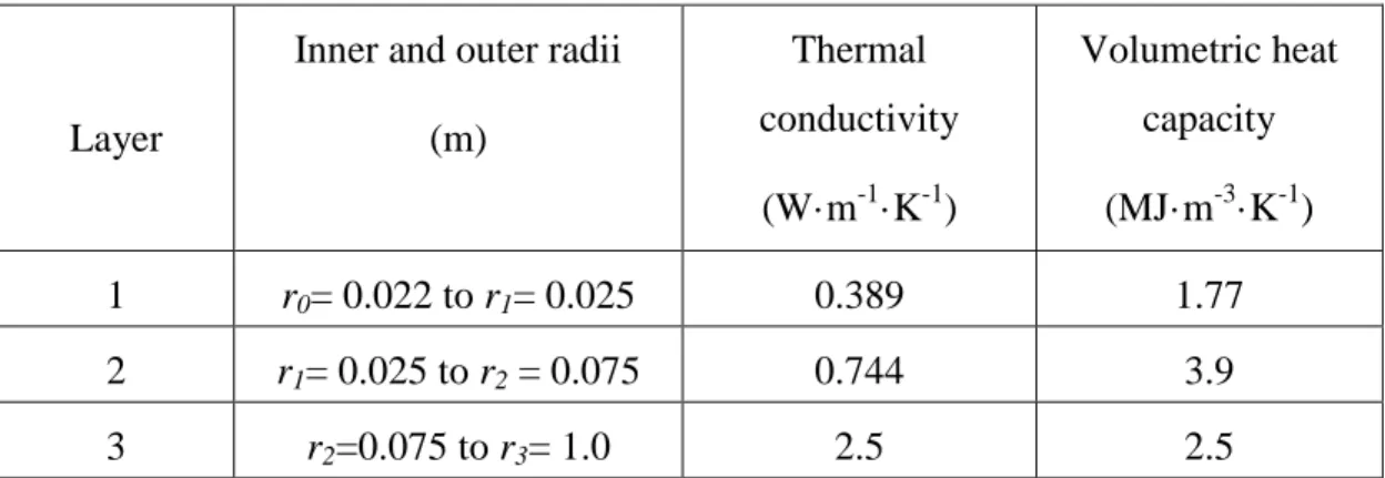
Table 2.1: Comparison between pipe and grout thermal capacities in typical boreholes. ... 30

Table 2.2: Characteristics of the composite cylinder used in the verification of the numerical code. ... 42

Table 2.3: Thermal properties and dimensions used for two test cases. ... 43

Table 2.4: Parameters used in the two test cases of the application section. ... 46

Table 2.5: Effect of accounting for thermal capacity on the annual heat pump COP. ... 55

Table 4.1: Coding system for all thermocouples. ... 82

Table 4.2: Thermal conductivities of the main components of the borehole. ... 84

(12)

LIST OF FIGURES

Figure 0.1: Schematic representation of a typical single U-tube ground heat exchanger. ... 2

Figure 0.2: Flow chart illustrating the work done in this study ... 5

Figure 1.1: Schematic representation of the infinite line source model. ... 7

Figure 1.2: Schematic representation of the finite line source model. ... 8

Figure 1.3: Schematic representation of the cylindrical heat source (CHS) method. ... 9

Figure 1.4: Schematic representation of the model proposed by Man et al. (2010). ... 10

Figure 1.5: Cross section of the buried cable used by Carslaw and Jaeger (1947). ... 11

Figure 1.6: Schematic representation of the geometry used by Lamarche and Beauchamp (2007). ... 12

Figure 1.7: Schematic representation of a 3 × 3 bore field. ... 13

Figure 2.1: Schematic representation of a typical single U-tube ground heat exchanger ... 22

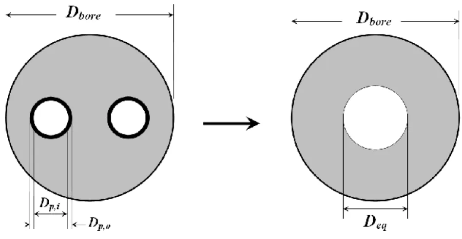
Figure 2.2: Representation of the transformation from a two-pipe geometry (Figure 2.1) to an equivalent single pipe. ... 29

Figure 2.3: Approximation of the real geometry with an equivalent cylinder with an equivalent inside diameter. ... 30

Figure 2.4: Schematic of the grids in the radial direction ... 34

Figure 2.5: Flow chart of the solution procedure. ... 40

Figure 2.6: Illustration of the calculation process in the proposed model ... 41

Figure 2.7: Comparison of the numerical solution with the steady-state analytical solution to heat transfer in a composite cylinder. ... 42

Figure 2.8: Comparison of the numerical solution with the transient analytical solution to heat transfer in a cylinder ... 44

Figure 2.9: Comparison between the proposed model and the experimental data of Spitler et al. (2009). ... 45

(13)

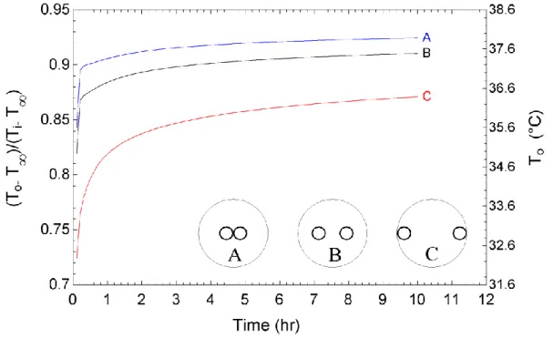
Figure 2.10: Transient behavior of three standard pipe configurations following a step change in

inlet temperature. ... 47

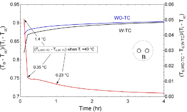
Figure 2.11: Non-dimensional outlet temperatures with and without thermal capacity effects. ... 48

Figure 2.12: Inlet temperatures to the borehole used in annual simulations. ... 50

Figure 2.13: Heat pump performance characteristics as a function of the inlet temperature. ... 50

Figure 2.14: Effect of borehole thermal capacity on the borehole outlet temperature. ... 51

Figure 2.15: Temperature profile for six consecutive time steps. ... 52

Figure 2.16: The temperature profile for seven consecutive time steps for frequent heat pump operation. ... 54

Figure 3.1: Schematic representation of the calculation domain. ... 58

Figure 3.2: Nomenclature used for the boundary conditions. ... 59

Figure 3.3: Schematic representation of an internal control volume in the calculation domain. ... 60

Figure 3.4: Modeling results comparison for case 1, t=.7200s. ... 62

Figure 3.5: Isotherms from the proposed numerical model for case 1 at t =7200s. ... 63

Figure 3.6: Modeling results, comparison for case 2 at t =7200s. ... 64

Figure 3.7: Geometry used for the proposed model (a) and for the FLS geometry (b). ... 65

Figure 3.8: Comparison of isotherms/results from the 2-D-model and the FLS solution after one day simulation time at the upper part of the domain/borehole. ... 67

Figure 3.9: Comparison of isotherms/results from the 2-D-model and the FLS solution after one day simulation time at the mid-part of the borehole. ... 68

Figure 3.10: Comparison of isotherms/results from the 2-D-model and the FLS solution after one day simulation time at the bottom part of the borehole. ... 69

Figure 4.1: Experimental apparatus. ... 71

Figure 4.2: Photos showing the assembly of the inlet and outlet temperatures measurement sections. ... 75

(14)

Figure 4.4: Concrete “cake” to fill the bottom curvature of the tank. ... 77

Figure 4.5: String rack. ... 77

Figure 4.6: Photos of the string rack construction. ... 78

Figure 4.7: Photos showing the fishing wires, a tension peg and the thermocouple fastening method. ... 79

Figure 4.8: Thermocouple numbering system. ... 81

Figure 4.9: Cross-section of the borehole used in the sand tank. ... 84

Figure 4.10: Photos showing various parts of the borehole. ... 85

Figure 4.11: Photos from the borehole and string rack. ... 86

Figure 4.12: Various temperatures and volumetric flow rate obtained during a preliminary experiment. ... 90

Figure 5.1: Isotherms showing the initial state of the temperature in the sand tank. ... 93

Figure 5.2: Measurements during the heat injection period. Inlet and outlet fluid temperature (top); volumetric flow rate (middle); ambient and far-filed temperatures (bottom). ... 94

Figure 5.3: Temporal evolution of temperature for azimuthal angles 0° and 180° ... 97

Figure 5.4: Temporal evolution of temperature for azimuthal angles 90° and 270° ... 98

Figure 5.5: Isotherms at t = 1 hour. ... 100

Figure 5.6: Isotherms at t = 72 hours. ... 101

Figure 5.7: Isotherms at t = 80 hours (7 hours after the end of the injection period). ... 102

Figure 5.8: Isotherms at t = 182 hours. ... 103

Figure 5.9: Temperatures at various azimuthal orientations during the heat injection period. .... 105

Figure 5.10: Comparison between experimental and numerical results at angle 0°. ... 108

Figure 5.11: Temperature evolution in time at angle 0° for R2, R3, and R4 for the first 20 hours of test. ... 109

(15)

Figure 5.12: Temperature evolution in time at angle 0° for R2, R3 and R4 during the recovery period as shown in Figure 5.10. ... 110 Figure 5.13: Comparison between experimental and numerical results at angle 90°. ... 111 Figure 5.14: Temperature profile at angle 0° and height of Z2 for heat injection period (top) and recovery period (bottom). ... 113 Figure 5.15: Temperature profile at angle 0° and R2 radial distance for heat injection period (top) and recovery period (bottom). ... 114

(16)

LIST OF APPENDICES

Appendix A: Time step and grid independence check. ... 129

Appendix B: Steady state analytical solutions to heat transfer from a cylinder. ... 132

Appendix C: Transient analytical solutions to heat transfer from a cylinder. ... 133

Appendix D: Calibration of temperature measurement probes. ... 134

(17)

NOMENCLATURE

a coefficient of the discretization equations

BC-B bottom boundary condition BC-L left boundary condition BC-R right boundary condition BC-T top boundary condition c specific heat (kJ/kg-K)

D half the centre-to-centre distance between pipes in the U-tube configuration (m)

Db borehole diameter (m)

Deq diameter of the equivalent pipe (m)

Dp diameter of U-tube pipes (m)

dt time step (s)

f flow meter output signal (Hz)

F0 Fourier number (Fogdt r/ bore2 )

G G-factor in the CHS method

h film coefficient (W/m2-K)

H overall height of the calculation domain for the proposed 2-D model (m)

int integer figure

IT internal time, number of intermediate calculations during each TI (-)

k thermal conductivity (W/m-K)

L active borehole length (m)

L1 vertical distance from ground surface to the top of borehole as shown in Figure 3.2 (m)

(18)

m measured mass (kg) m mass flow rate (kg/s)

NI number of calculations done in the numerical borehole model during each RT (-)

q’ rate of heat transfer per unit length at the equivalent pipe wall (W/m)

q” heat flux imposed at the inner pipe wall (W/m2)

r radial distance from the borehole center (m)

rb borehole radius (m)

req equivalent pipe radius = Deq/2 (m)

rp pipe radius of the U-tubes pipes (m)

Rb,ss steady state borehole thermal resistance for the real single U-tube borehole geometry

(K-m/W)

RT residence time Figure 2.5

t time (s)

tres residence time (s), given by Equation (2.5)

T temperature (°C)

TI time increment, the time between two step changes in inlet conditions (s)

Ti inlet fluid temperature to the borehole (ºC)

Tm mean fluid temperature = (Ti+ To)/2 (ºC)

To outlet fluid temperature from the borehole (ºC) eq

r

T temperature at req (ºC)

Tw borehole wall temperature (ºC)

u fluid velocity (m/s)

U uncertainty

(19)

Subscripts

bore associated with the borehole wall b bottom neighbor

e east neighbor

eq associated with the equivalent diameter pipe

f fluid

gd ground

gt grout

i internal, inlet

in internal (for internal radius in Chapter 3)

n north neighbor

o external, outlet

p associated with the U-tube pipes also denotes point in discretization equations

real associated with the real U-tube configuration

eq associated with the equivalent pipe wall

s south neighbor t top neighbor w west neighbor ∞ far field

Superscripts

0

value at the preceding time step

Greek letters

α thermal diffusivity (m2/s)

(20)

δz axial distance between two control-volume faces (m) Δr radial increment (m)

Δzr axial increment (m) Δt time step (s)

θ temperature at a particular radial distance minus that of the far field; θ(r,t)=T(r,t)-T∞ (ºC)

σ standard deviation

ρ density (kg/m3)

Abbreviations

1-D one dimensional

2-D two dimensional

CHS cylindrical heat source COP coefficient of performance DST duct ground heat storage model FLS finite line source

GCHP ground coupled heat pump GHE ground heat exchanger GSHP ground source heat pump HDPE high density polyethylene ILS infinite line source

TC thermocouple

TCI-IN T-type hollow tube thermocouple measuring fluid temperature at inlet side TCI-OUT T-type hollow tube thermocouple measuring fluid temperature at outlet side

(21)

INTRODUCTION

Background and generalities

The energy consumed in residential and commercial/institutional buildings account for almost 30 percent of the total annual energy consumption in Canada (NRCan, 2006). Approximately 60 percent of this amount is used for space heating and cooling. A recent report by The National Round Table on the Environment and the Economy and Sustainable Development Technology Canada indicates that the commercial building sector is accountable for 14% of the end-use energy consumption and for 13% of the carbon emissions in Canada. Furthermore, the recent environmental ambition to reduce carbon emissions has given rise to extensive research on alternative, low-cost energy sources and on energy efficiency measures.

Ground coupled heat pump systems are energy-efficient, environment friendly and sustainable alternatives (Nouanegue et al. (2009)) to conventional systems. In general, these systems collect (or reject) heat through ground heat exchangers which can be installed either vertically or horizontally. This research concentrates on vertical systems.

A schematic representation of a vertical ground heat exchanger (GHE) is shown in Figure 0.1. It consists of a borehole in which a U-tube pipe has been inserted. The borehole is usually filled with a grout to enhance heat transfer by providing good thermal contact between the fluid and the ground. The grout is also used to protect underground aquifers. The depth of the borehole (L) is approximately 100 m (328 ft) and its diameter is usually in the 10-15 cm range (4 to 6 inches) while the inside diameter of the U-tube pipes is approximately 25 mm (1 inch). High density polyethylene (HDPE) pipes are used for the U-tubes. The center-to-center distance between these pipes varies from cases where the pipes are touching each other to cases where the pipes are touching the borehole wall on opposite sides. A fluid is pumped into the U-tube. In heating, the fluid has a lower temperature than the ground and heat is transferred from the ground to the fluid. In cooling, heat transfer is in the opposite direction as the fluid is at a higher temperature than the ground. The borehole can experience a variety of flow rates ranging from no flow to full flow conditions and any flow in between if the system is equipped with a variable flow pumping system. At full flow, the residence time, i.e., the time required for the fluid to travel from the inlet to the outlet, is of the order of a few minutes. The temperature difference between the inlet (Ti)

(22)

and outlet (To) temperatures will vary according to the flow rate with typical values around 5 ºC

(9 ºF).

Figure 0.1: Schematic representation of a typical single U-tube ground heat exchanger. Variations in the inlet conditions (either temperature or flow) do not translate immediately into a similar change in the outlet conditions. This is due to two main reasons. First, the residence time of the fluid in the borehole creates a delay. Second, any changes at the inlet are dampened by the fluid and grout thermal capacities.

Problem definition

Determination of the length of the geothermal heat exchanger is one of the fundamental issues in designing a reliable ground coupled heat pump system. Over estimation of the GHE length leads to high installation costs while under-sizing may lead to operational problems resulting from

(23)

ground return fluid temperature that are outside the heat pump operating range. Accurate prediction of the outlet fluid temperature from the borehole is important for design purposes, building annual energy simulations and estimation of the heat pump energy consumption. Therefore, accurate heat transfer predictions in and around boreholes is important.

In general, ground heat exchanger models are divided into two distinct regions each with its own time scale with rapid changes inside the borehole and slow variations of ground temperature far away from the borehole. The current study concentrates on the borehole and its immediate vicinity. There are a number of borehole models in the literature that can be used to predict the thermal behavior of boreholes. With a few exceptions, most of these models are steady-state models which neglect the thermal capacity of the boreholes by simply replacing the borehole with a steady-state thermal resistance. While this assumption might be acceptable if the heat pump operates continuously, it is questionable when heat pumps undergo on/off cycles to meet the building load. A paucity of information in the literature has been identified in two areas. First, the effects of grout thermal capacity on the annual energy consumption of heat pumps have not been studied extensively. Second, field-monitored data are usually inadequate for precise model validation and there is a lack of good experimental data obtained in controlled conditions. Given these gaps in the literature, this work was undertaken with the following objectives.

Objectives

The objectives of this study are to:

1. develop a computationally efficient transient one-dimensional model that accounts for grout and fluid thermal capacity that could be incorporated in energy simulation programs;

2. develop a two-dimensional numerical model of the ground in the vicinity of boreholes; 3. design and construct a small-scale experimental apparatus to validate the current models

(24)

Organization of this thesis

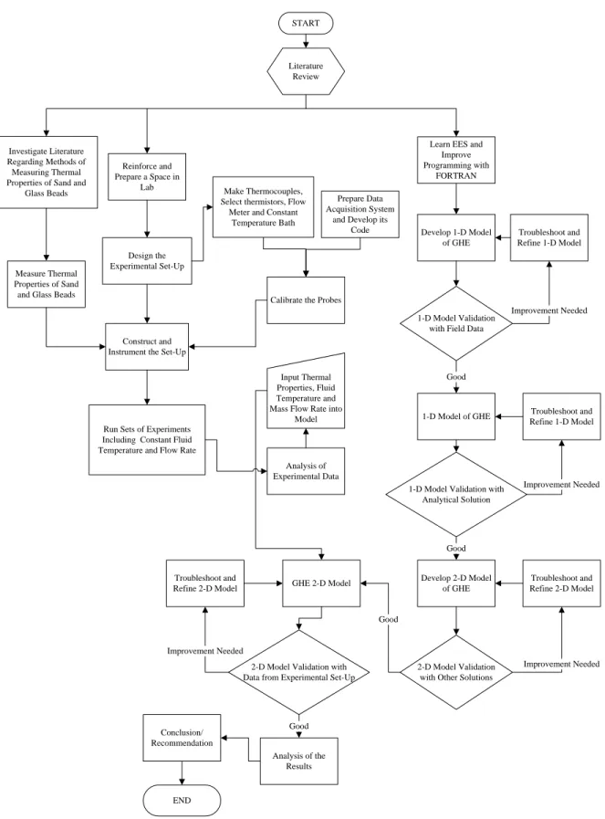
Aside from the introduction and conclusion, this thesis is structured around five chapters and five appendices. Chapter 1 addresses previous research considered relevant to this study. The hybrid one-dimensional transient model is presented in Chapter 2 along with results on the impact of borehole thermal capacity on the annual heat pump energy consumption. It should be noted that Chapter 2 has been submitted to a journal for publication. A two-dimensional numerical model of the ground is presented in Chapter 3; verifications with other solutions are provided. Chapter 4 describes the experimental set-up and the results of a preliminary experiment. The final set of experimental results is presented in Chapter 5 including comparisons with the model developed in Chapter 3. A detailed flowchart is presented in Figure 0.2 to illustrate the various steps undertaken during the course of this study.

(25)

START Literature

Review

Learn EES and Improve Programming with FORTRAN Develop 1-D Model of GHE 1-D Model Validation with Field Data

Troubleshoot and Refine 1-D Model Reinforce and Prepare a Space in Lab Design the Experimental Set-Up Construct and Instrument the Set-Up

Prepare Data Acquisition System

and Develop its Code Make Thermocouples,

Select thermistors, Flow Meter and Constant

Temperature Bath

Calibrate the Probes

Run Sets of Experiments Including Constant Fluid Temperature and Flow Rate

1-D Model Validation with Analytical Solution Investigate Literature

Regarding Methods of Measuring Thermal Properties of Sand and

Glass Beads

Improvement Needed Measure Thermal

Properties of Sand and Glass Beads

Input Thermal Properties, Fluid Temperature and Mass Flow Rate into

Model 1-D Model of GHE Good Troubleshoot and Refine 1-D Model Improvement Needed Analysis of Experimental Data Develop 2-D Model of GHE 2-D Model Validation with Other Solutions

Troubleshoot and Refine 2-D Model GHE 2-D Model Good Improvement Needed Good

2-D Model Validation with Data from Experimental Set-Up Troubleshoot and Refine 2-D Model Improvement Needed Analysis of the Results Conclusion/ Recommendation END Good

(26)

CHAPTER 1 LITERATURE REVIEW

1.1 Introduction

Transient heat transfer inside and in the vicinity of vertical ground heat exchangers (GHE) is the main focus of this thesis. Existing models used for analyzing vertical GHE are described in this chapter. First, a brief review of some of the fundamental studies on ground heat transfer for boreholes and bore field is presented. Then, previous works related to modeling of GHE is reviewed.

1.2 Fundamental studies on ground heat transfer

There are two major analytical solutions to the transient heat transfer equation in cylindrical coordinates. They are referred to as the line source (either infinite of finite) and the cylindrical heat source solutions. A brief review of these solutions is presented in the following paragraphs.

1.2.1 Infinite line source (ILS) method

The line source theory, first introduced by Lord Kelvin in 1882, is considered as one of the most basic analytical transient one-dimensional solutions which can be used for geothermal applications. As schematically shown in Figure 1.1, the borehole geometry is approximated by an infinite line source/sink surrounded by an infinite homogeneous medium (i.e., ground). Pure heat conduction in the ground is assumed and the solution is one-dimensional in the radial direction. When using the ILS it should be realised that the heat transfer rate is applied at the center of the borehole. The time it takes for a heat impulse at the center to reach steady-state at the borehole wall (for Db/2 = rb ≈ 5 to 7.5 cm) has been evaluated by Eskilson (1987) to be equal to 5rb2/α,

where α is the thermal diffusivity of the ground. This time, which is typically 3 to 6 hours, corresponds to the time at which the difference between accurate models (such as the g-function) and the infinite line source (ILS) solution falls below 10 %. Ingersoll et al. (1954) proposed a lower time limit of 20rb2/α, which corresponds to a difference of 3 % according to Philippe et al.

(2009). For long operating times (typically of the order of a year), axial heat conduction is significant and the ILS model becomes imprecise.

(27)

Figure 1.1: Schematic representation of the infinite line source model.

1.2.2 Finite-line source (FLS) method

Eskilson (1987), Diao et al. (2004) and Zeng et al. (2002) developed an explicit solution of a finite line-source to express more accurately the two dimensional temperature response (radial and along the length of the borehole) of vertical boreholes submitted to a uniform heat transfer rate per unit length in a semi-infinite homogeneous constant-property ground, as schematically shown in Figure 1.2. The FLS will be described further in Chapter 3 in conjunction with the presentation of the proposed two-dimensional ground model.

(28)

Figure 1.2: Schematic representation of the finite line source model.

1.2.3 Cylindrical heat source (CHS) method

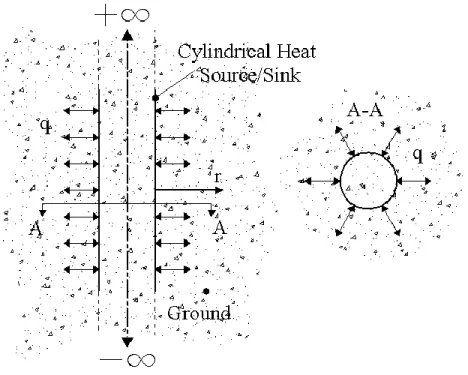
One convenient and simple method of evaluating ground heat transfer is to use the so-called cylindrical heat source (CHS) method which was originally proposed by Ingersoll (1954), based on the work of Carslaw and Jaeger (1947). The CHS method, as shown in Figure 1.3, is based on the analytical solution to transient heat transfer from a cylinder embedded in an infinite homogeneous medium. The CHS solution for constant heat transfer rate is given in terms of a G-factor which depends on Fo, the Fourier number, and p (where p is the ratio of the radius where

the point of interest is located over the radius of the borehole). The solution to the G-factor involves the solution of a relatively complex integral (Bernier, 2000 ; Bernier, 2001). Fortunately, tabulated values of G are available for p=1, 2, 5,and 10 Ingersoll (1954). In addition, Bernier and Salim Shirazi (2007) have recently proposed G-factor correlations for p = 20, 50 and 100. The CHS method suffers form its inherent one-dimensional nature and like the line source method it becomes inaccurate for long operating time when axial conduction becomes significant. According to the recent work of Sheriff (2007) axial conduction starts to be significant for αt/r2 > 104 .

(29)

Figure 1.3: Schematic representation of the cylindrical heat source (CHS) method.

Philippe et al. (2009) compared the infinite line source, the infinite cylindrical source and the finite line source models and a validity map was presented for typical operating conditions. They showed that if the relative error of the borehole wall temperature is to be kept below a certain value, say 2%, the infinite line source model can be applied after 34 hours and up to 1.6 years of operation. For operation time below 34 hours, the infinite cylindrical source is recommended to stay below the same level of error. After 1.6 years of operation, the two-dimensional effects become significant and the finite line source should be used.

1.2.4 Other analytical approaches

Man et al. (2010) proposed analytical models for 1D and 2D solid cylindrical heat sources (with infinite and finite vertical dimension, respectively) which can be used for modeling pile GHEs with spiral coils. The models take the simplifying assumption of replacing the spiral heating coil with a continuous cylindrical heat source with no thickness, mass or heat capacity as shown in Figure 1.4. They account for the heat capacity of the borehole or pile by assuming a homogeneous medium for the whole calculation domain including the solid cylindrical region

(30)

inside the pile. The infinite heat source model was compared by the authors against the classical line source and “hollow” cylindrical source models.

Figure 1.4: Schematic representation of the model proposed by Man et al. (2010).

An analytical solution to the heat flow from an infinite buried cable to its surrounding ground was proposed by Carslaw and Jaeger (1947). As illustrated in Figure 1.5, the cable consists of the following layers: a metal core, insulation and an outer protective sheath. Unlike the line source and cylindrical heat source methods, the buried cable model takes into account the thermal capacities of the metal core and protective sheath. However, their thermal resistances are ignored due to their high thermal conductivities. On the other hand, the thermal resistance of the insulation ring is accounted for while its thermal capacity is neglected.

(31)

Figure 1.5: Cross section of the buried cable used by Carslaw and Jaeger (1947).

An analytical approach for evaluating the short time response of boreholes, based on the buried cable solution, is proposed by Young (2001). In that solution, the electrical cable consists of a current carrying core separated from a metal sheath by insulation which acts as a contact thermal resistance. By analogy, Young replaced the core with the working fluid and the metal sheath with grout thermal capacity. The contact resistance represents the steady state thermal resistance. It is expressed using the multipole approach proposed by Bennet et al. (1987). To improve the accuracy of the model, Young considered moving part of the grout thermal capacity from the outside of the thermal resistance to the inside by introducing a grout allocation factor, GAF. The total thermal mass of the working fluid was taken into account. It included the thermal mass of the fluid inside the U-tube as well as in the distribution piping system connected to the GHEs. The goal was to study the effect of the total fluid thermal mass on the working fluid temperature during the peak loads as well as the impact of the peak load duration on the fluid temperature in peak load dominant buildings such as churches. This effect was introduced using a fluid

(32)

multiplication factor. It was shown that the choice of the fluid multiplication factor has an important impact on the GHE design.

After examining and comparing several existing steady state methods, Young concluded that the method chosen to calculate the borehole thermal resistance has also a significant effect on the estimated length of the GHE. Among available methods, the multipole method of Bennet et al. (1987) was selected as the best analytical steady state approach. Young indicated that the grout thermal resistance was highly sensitive to the U-tube diameter, shank spacing between the U-tube pipes, borehole diameter, as well as the grout and ground thermal conductivities. When the U-tube legs touch the borehole wall, the thermal mass of the grout has less of an impact as most of the heat can be transferred directly to the ground. Young compared his model against the line source model for an hourly annual simulation of a small office building. He concluded that the heat pump energy consumption calculated by the line source model is as precise as his proposed model. Yet, Young mentioned that for short duration peak loads, line source over predicts the peak outlet fluid temperature from the borehole by as much as 1.3ºC.

Figure 1.6: Schematic representation of the geometry used by Lamarche and Beauchamp (2007). Using the method of optimal linearization, with the initial solution given by the integral method, Kandula (2010) presented a closed form approximate solution of the transient temperature distribution in a hollow cylinder with a linear variation of thermal conductivity with temperature. The boundary conditions are convective heating at the exposed inner surface while the outer

(33)

surface is adiabatic. The non-linear analytical solution compares well with the finite difference numerical solution.

1.3 Bore field models

As schematically shown in Figure 1.7, some installations have more than one borehole. Analytical solutions such as the ones presented in the previous section have to be superimposed in space when there is borehole thermal interference in a bore field (Chapuis, 2009). Two of the most popular approaches to model bore fields are the g-function concept introduced by Eskilson (1987) and the DST model from Hellström (1991). These two approaches will now be briefly reviewed.

Figure 1.7: Schematic representation of a 3 × 3 bore field.

Eskilson’s model calculates the average borehole wall temperature in a bore field using numerical solution techniques. Only heat transfer in the ground is considered and heat transfer inside the borehole has to be accounted for using another model. The numerical model solves the governing equations in a radial-axial cylindrical coordinate system using the finite difference method. A

(34)

spatial superimposition technique is used to obtain the response of the whole bore field. The g-functions which are a set of non-dimensional temperature response factors are derived from the temperature response of the bore field. The g-functions facilitate the calculation of the temperature change at the borehole wall corresponding to a step heat input. Once the response of the bore field to a single step heat pulse is represented by a g-function, its response to any heat rejection/extraction function can be determined by simply converting the heat rejection/extraction into a set of step functions and superimposing the response to each step function. The g-functions are presented as curves, plotted versus non-dimensional time, ln(t/ts), where ts = H2/(9α) is the

time scale and H is the borehole vertical length. Each g-function curve corresponds to a particular

rb/H, where rb is the borehole radius, and a single B/H where B is the distance between the

boreholes. As the number of boreholes increases, the thermal interaction between them becomes stronger especially for long operating time periods. For short operating times, Eskilson considers the g-functions to be valid for times greater than 5(rb)2/α .

Hellström (1991) developed a three dimensional simulation model for seasonal thermal energy storage equipped with ground source heat exchangers. The storage temperature is calculated by considering the following three components: a local solution, a global temperature and a steady flux solution. The local component takes into account the convective rate of heat transfer from the circulating fluid to the heat store volume while the global component considers the conductive heat transfer between the boreholes and the cylindrical volume by implementing the temperature difference between the heat store volume and the undisturbed ground temperature. These two solutions are obtained using an explicit finite difference approach. The steady flux component which takes into account the distribution of the heat coming from the fluid to the borehole and then diffusing to the cylindrical soil volume is determined analytically. Finally, the ground temperature distribution is obtained through superposition methods. Hellström’s model, also known as the DST model, has been implemented in TRNSYS. It is considered one of the most accurate bore field models. The reader is referred to the work of Chapuis (2009) and Chapuis and Bernier (2009) for a complete description of the DST model.

(35)

1.4 Heat transfer modeling inside the borehole

This section reviews heat transfer models for the inside of the borehole. Other papers on the same subject, but more pertinent to Chapter 2, are included in that chapter.

Some early but fundamental work on borehole modeling was done by Kavanaugh (1985). In his work, he determined the rate of heat transfer or the temperature distribution around a buried pipe in the ground using the cylindrical heat source solution. He developed the cylindrical heat source approach considering a single isolated pipe surrounded by an infinite solid (soil) having constant properties. Kavanaugh also makes some adjustments to the cylindrical heat source approach to get a better match with his experimental data. Deerman and Kavanaugh (1991) extended the cylindrical heat source model to account for variable heat transfer rates. However, their approach is not suitable for the analysis of short-term field data. Kavanaugh, proposed an equivalent single pipe instead of a U-tube. The equivalent diameter approximates the U-tube geometry and is calculated using D_eq  n D( _o) where n is the number of U-tube legs (2 for a single U-tube). Muraya et al. (1996) developed a transient two-dimensional finite element model for single U-tube boreholes to analyze thermal interaction between the two pipes of the U-U-tube. Defining a heat exchanger effectiveness, the thermal interference was quantified by investigating the impacts of the shank spacing, U-tube leg temperatures, ground temperature and backfills. The problem was solved numerically and it was found that the shank spacing and backfill thermal conductivity had the most significant influence on the effectiveness results. To properly account for the backfill thermal conductivity, the effectiveness had to be modified. They reported that the overall heat transfer to the ground can be increased by increasing the shank spacing and backfill thermal conductivity.

Remund (1999) proposed a set of relationships, based on the concept of conduction shape factors, to calculate steady-state borehole thermal resistances. Empirically-based coefficients are presented for three single U-tube borehole configurations, often referred to as the A, B, and C, configurations. It should be mentioned that in the proposed relations, the convection resistance on the inside pipe wall is not included. The Remund relationships are often used because of their simplicity.

(36)

Yavuzturk and Spitler (2001) used actual operational field data from an elementary school to validate their short time step temperature response factor model. Reasonable agreement was reported between the measured data and the short time step model, despite some shortcomings in the experimental data set. The predicted entering fluid temperature to the heat pump shows maximum deviation relative to the measured data when the fluid flow rate is discontinuous. Lee and Lam (2008) studied the performance of ground heat exchangers and proposed a three- dimensional model using the implicit finite difference method in rectangular coordinates. The model approximates each borehole as a square column circumscribed by the borehole radius. Their approach can handle variable temperature and loading along the borehole. However, quasi-steady state heat transfer is assumed inside the borehole. Comparison has been done between simulation results from their model and those of the finite line source as well as cylindrical heat source method.

Cui et al. (2008) developed a finite element numerical model for simulating GHEs in alternative operation modes over a short time period for GCHP applications. It was concluded that for short time scale simulations, the proposed model is more suitable than the line source model.

Bandyopadhyay et al. (2008a) developed a one-dimensional (radial) analytical solution for the transient heat transfer from cylinder in homogeneous media. In order to take into account the thermal capacity of the working fluid, the proposed approach considers it as a “heat generating” virtual solid, VS, which is in direct contact with the grout medium through a thermal contact conductance. A finite element model was used for comparison. By varying the Biot number and comparing the analytical results of fluid temperature with those of the finite element model, they extended the solution to the U-tube geometry. Good agreement was reported for the case where the two pipes of the U-tube were in close contact. In a related article, Bandyopadhyay et al. (2008b) obtained a semi-analytical solution for the short time transient response of a grouted borehole subjected to a constant internal heat generation rate. Using numerical algorithms, the average fluid temperature as well as the borehole wall temperature have been obtained and compared against their corresponding simulated results from finite element models of the actual single U-tube grouted boreholes. Good agreement is reported between the numerical results for boreholes with touching pipes against the results obtain from the proposed method using a single equivalent core. Sensitivity analysis has been done for several non-touching pipes while varying

(37)

the Biot number in order to reach a better agreement between the numerical and proposed approaches.

Li and Zheng (2009) introduced a three dimensional unstructured finite volume numerical model of a GHE using a Delaunay mesh generator to capture the geometry of the borehole. The model takes the inlet fluid temperature to the GHE together with volumetric flow rate as input to calculate the outlet fluid temperature. Experimental data (i.e., inlet and outlet fluid temperature) from a so-called ground sink direct cooling system (GSDCS) operating on an intermittent mode (12 hours on, 12 hours off) is used to verify the proposed numerical model. The flow rate is considered to be constant during the whole on-cycle period. The numerical model neglects the conductive heat transfer along the fluid as well as the pipe thermal capacity. The bottom boundary condition is imposed at the bottom of the borehole thus neglecting end effects. Similarly, the top boundary condition is imposed at the ground surface where the top of the borehole is assumed to be located. Hourly comparison curves have been presented showing relatively good agreement between the numerical results and the experimental data except at the start of the operation.

Javed et al. (2009) reviewed and compared several analytical and hybrid models for vertical GHE for short and long term analysis. They addressed the strengths and limitations of these models and concluded that there is a shortage of analytical models when it comes to bore fields. There is also a need for proper analytical models for simulating both the short and long term response of GHEs without distorting the actual borehole geometry.

De Carli et al. (2010) developed a model to simulate the thermal behavior of vertical GHEs based on the electrical analogy using thermal resistances and lumped capacities to solve the unsteady heat transfer phenomenon. The model is capable of simulating three pipe arrangements commonly found in GHEs: single U-tube, double U-tube and coaxial pipe. The simulation domain is divided into a number of overlapped slices in the vertical direction with each slice subdivided into a number of annular regions. Heat transfer between two vertical slices in the vertical direction is neglected and only the heat flux along the radial direction is considered. The borehole thermal capacity (fluid, pipe, and grout) is not taken into account. For the flow, the mean fluid temperature is assumed to have the same value as the outlet fluid temperature in a particular vertical slice. Making these assumptions, the flow temperature profile and ground

(38)

temperature at different radial and vertical distances can be determined. Comparison has been done between measured and simulated results and good agreement is reported.

In a recent review article, Lamarche et al. (2010) compared different existing approaches to calculate borehole thermal resistance including the thermal short-circuit between the U-tube pipes. An unsteady 3-D numerical simulation of a single U-tube borehole was performed and good agreement was reported between the axial fluid temperature distribution of a single U-tube borehole obtained from the approach proposed by Zeng et al. (2003) and that of the three-dimensional simulation.

Oppelt et al. (2010) proposed a steady-state model for the grout region inside a certain type of parallel double U-tube configuration. The numerical domain in the vertical direction is divided into a number of non-conducting slices. The grout region of each slice is divided into three elements each one representing a certain temperature zone. The proposed model was combined with an existing model to calculate the temperature distribution within the ground and the fluid. Annual simulations of heat pump operation with a time step of one hour are possible with this model. Comparison has been done between the outlet fluid temperature from the “combined” proposed model against that of a 3D numerical model (developed in ANSYS CFX) during heat pump operation for three different pipe spacings. The comparison showed relatively good agreement especially for the case where the pipes were equally distanced from the borehole center and borehole wall. The proposed model proved to be faster in terms of simulation time compared to the numerical model.

Zeng et al. (2003), based on Hellström’s work, established a quasi-three dimensional analytical steady-state solution for single and double U-tube configurations arranged either in series or in parallel. The axial temperature variation along the length of the U-tube can be predicted. This study shows that the double U-tube configuration provides a larger heat transfer area between the flowing fluid and the grout leading to a smaller borehole resistance. For double U-tubes BHEs, the parallel arrangement is suggested. Their results show that increasing the U-tube shank spacing decreases the borehole resistance noticeably. Equivalent borehole thermal resistances are proposed for several combinations of circuit arrangement. Their models also account for thermal interaction between U-tube legs. Diao et al. (2004) adopted the analytical borehole model of Zeng

(39)

et al. (2003) and combined it with the finite-line source model to simulate the heat transfer phenomenon inside the borehole as well as its surrounding ground.

Marcotte and Pasquier (2008) proposed a “p-linear” average temperature using a three-dimensional numerical simulation to estimate the borehole thermal resistance from a thermal response test. It was reported that the assumptions of constant heat flux along the borehole length or constant borehole wall temperature lead to an overestimation of the borehole thermal resistance and consequently to the borehole length. The economic impact of an oversized borehole length was evaluated in a case study with multiple boreholes.

Marcotte et al. (2010) examined the effects of axial heat conduction in boreholes comparing results obtained from the finite and infinite line source solutions. Presenting simulation results for an unbalanced annual load, two cases with different ratio of borehole spacing over borehole length were studied. One of the main conclusion is that the greater this ratio, the more significant the axial effects are while determining the total number of boreholes required in a bore field. Beier (2011) proposed an analytical model of the actual vertical temperature profile in a GHE for the late-time period of an in-situ test. With this method, one can estimate the ground thermal conductivity as well as the borehole thermal resistance without using the usual average fluid temperature approximation. A sensitivity study based on the vertical fluid temperature profile model has been carried out which shows the errors associated with making the mean fluid temperature approximation assumption while estimating the borehole resistance. Their research proposes to use the p-linear average method of Marcotte and Pasquier (2008) over the usual mean temperature approximation.

Du and Chen (2011) also proposed the use of a p-linear dimensionless fluid temperature to estimate the steady-state fluid temperature and the borehole thermal resistance. Comparison with results from a quasi-three-dimensional model for single and double U-tube boreholes lead to suggested p values for the proper estimation of the thermal resistance.

Beier et al. (2011) constructed an 18 m long laboratory sandbox filled with saturated sand to generate reference data sets for a single U-tube borehole under controlled conditions. An aluminum tube is used as the borehole wall. The inside is filled with a grout and includes a HDPE U-tube with spacers. Much like the experimental set-up used in the present work, they measured sand temperatures at several locations including the borehole wall. Thermistors are installed in

(40)

the sand on the horizontal plane that runs through the centerline of the U-tube, all on the inlet side. Two other thermistors measure the inlet-outlet fluid temperatures. A thermal response test was carried out with a steady heat input to determine the ground thermal conductivity as well as the borehole thermal resistance

Recently, Claesson and Hellström (2011) revised and expanded the multipole method to evaluate the steady state heat transfer between a set of arbitrarily positioned circular pipes inside a composite cylindrical region. The proposed method calculates the local thermal resistances between the working fluid in the borehole and the ground in the immediate vicinity of the borehole. The classic Multipole method is improved by replacing the constant temperature condition at a circle outside the borehole by an average radial temperature. In fact, averaged temperature is prescribed at the borehole wall as the outer boundary condition. Also, instead of starting the analysis with prescribed fluid temperatures, prescribed heat fluxes are implemented. Pasquier and Marcotte (2012) improved the thermal resistance capacity model (TRCM) of Bauer et al. (2011) to integrate the thermal capacities of the working fluid and the pipe. Comparison is done between their proposed approach against a numerical model (which does not account for the fluid thermal capacity). Good agreement between the two models at short and late simulation times is achieved. However, the comparison is not as good for intermediate times. It should be mentioned that the fluid temperature of the inlet and outlet pipes are assumed to be constant over time.

(41)

CHAPTER 2 THERMAL CAPACITY EFFECTS IN BOREHOLE

GROUND HEAT EXCHANGERS

2.1 Introduction

This chapter reproduces the content of a journal article submitted to Energy and Buildings (Salim Shirazi and Bernier, 2012). The review presented in section 2.3 complements the literature review presented in Chapter 1.

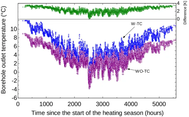
In this article, a one-dimensional transient borehole model is proposed to account for fluid and grout thermal capacities in borehole ground heat exchangers with the objective of predicting the outlet fluid temperature for varying inlet temperature and flow rate. The standard two-pipe configuration is replaced with an equivalent geometry consisting of a single pipe and a cylinder core filled with grout. Transient radial heat transfer in the grout is solved numerically while the ground outside the borehole is treated analytically using the cylindrical heat source method. The proposed model is validated successfully against analytical solutions and experimental results. For a typical two-pipe configuration, it is shown that the fluid outlet temperature predicted with and without borehole thermal capacity differ by 1.4, 0.35, and 0.23 °C after 0.1, 0.2 and 1 hour, respectively. Annual simulations are also performed over an entire heating season (5600 hours) with a 6 minute time step. Results show that the outlet fluid temperature is always higher when borehole thermal capacity is included. Furthermore, the difference in fluid outlet temperature prediction with and without borehole thermal capacity increases when the heat pump operates infrequently. The end result is that the annual COP predicted is approximately 4.5% higher when borehole thermal capacity is included.

2.2 Problem statement

Closed-loop ground coupled heat pump systems rely on ground heat exchangers (GHE) to reject or extract heat from the ground. A schematic representation of such a heat exchanger is shown in Figure 2.1. It consists of a borehole in which a U-tube pipe is inserted. The borehole is usually filled with a grout to enhance heat transfer and protect underground aquifers. In general, the depth of the borehole (L) is approximately 100 m (328 ft) and its diameter is usually in the 10-15 cm range (4 to 6 inches). High density polyethylene (HDPE) pipes are typically used for the

(42)

U-tubes. The inside diameter of these pipes is approximately 25 mm (1 inch). The center-to-center distance between these pipes varies from cases where the pipes are touching each other in the center of the borehole to cases where the pipes are touching the borehole wall on opposite sides. These two cases are often referred to as the A and C configurations (Remund (1999)). In the B configuration (shown in Figure 2.1), the pipes are equally distanced from each other and from the borehole wall.

Figure 2.1: Schematic representation of a typical single U-tube ground heat exchanger Heat is transferred from the fluid circulating in the pipes to the ground. The borehole can experience a variety of flow rates ranging from no flow to full flow conditions and any flow in between if the system is equipped with a variable flow pumping system. At full flow, the residence time, i.e., the time required for the fluid to travel from the inlet to the outlet, is of the order of a few minutes. The difference between the inlet (Ti) and outlet (To) temperatures is

typically around 5 ºC (9 ºF). Inlet conditions (either temperature or flow) variations do not lead to instantaneous changes in the outlet conditions. This is due to two main reasons. First, the

(43)

residence time of the fluid in the borehole induces a delay. Second, any changes at the inlet are dampened by the fluid and grout thermal capacities.

Ground heat exchangers can be modeled in two distinct regions: from the fluid to the borehole wall, and from the borehole wall to the far field. Ground models have been the subject of many investigations including a comparison exercise (Bernier et al. (2007)). The present study concentrates on the inside of the borehole. A one-dimensional transient borehole model is proposed to account for fluid and grout thermal capacities. The objective is to accurately predict the outlet fluid temperature for varying inlet conditions so that borehole thermal capacity can be accounted for in energy simulation programs. The borehole model is coupled here to a ground model which is based on the cylindrical heat source method.

2.3 Review of previous studies

Some of the important pioneering works can be attributed to Eskilson (1987) and Hellström (1991). Using spatial superposition, Hellström developed a 3-D simulation model for borehole thermal energy storage systems. The model was implemented in the TRNSYS (2006) simulation program by Hellström el al. (1996). However, the thermal capacity of the borehole is not included in the model. When there is flow in the borehole, the fluid temperature is evaluated using the borehole wall temperature and a steady-state thermal resistance. For no flow conditions, the fluid temperature is set equal to the borehole wall temperature.

Eskilson’s model calculates the average borehole temperature in a bore field using numerically generated g-functions. It is important to note that the borehole thermal capacity is not accounted for in the original g-functions and that heat transfer to the ground is applied at the borehole wall. Therefore, if only the heat transfer rate in the fluid is known, then one has to evaluate the time it takes for a heat impulse in the fluid to reach steady-state at the borehole wall in order to properly use g-functions. This time has been evaluated by Eskilson to be equal to tb = 5rb2/αg, where rb is

the borehole radius and αg is the thermal diffusivity of the grout material. For typical boreholes,

tb is of the order of 3 to 6 hours (Yavuzturk and Spitler (1999)).

Wetter and Huber (1997) modeled the transient behavior of a single borehole with a double U-tube configuration. This model was implemented in TRNSYS as Type 451. It accounts for grout thermal capacity as well as fluid thermal capacity. In the radial direction, heat transfer is

(44)

simulated numerically from the borehole center up to a distance of two meters where the boundary temperature is evaluated using Kelvin’s line-source solution. The four-pipe geometry is transformed into a single pipe of equivalent diameter centrally located in the borehole. The grid spacing is non-uniform in the radial direction with one grid point located in the equivalent annulus representing the grout. In the axial direction, the computational domain is subdivided into several ground layers. The fluid temperature is calculated numerically in each of these layers using a transient energy balance.

Rottmayer et al. (1997) proposed a finite difference model to simulate a vertical ground heat exchanger. The model combines the borehole as well as the adjacent ground. It solves the three-dimensional transient problem using the explicit finite difference approach in cylindrical coordinates. The thermal capacity of the fluid is taken into account but it is assumed that pipe and grout thermal capacities can be neglected. The authors justify the use of this assumption by claiming that "the thermal energy change of the grout over a year is on the order of 0.5% of the total heat flow, and thus the wall and grout capacitances are not significant in annual simulations".

Gu and O'Neal (1998) developed an analytical solution to obtain the transient temperature response in a composite media (grout and surrounding ground). Using an equivalent pipe diameter, the governing one-dimensional radial equation is solved using a generalized orthogonal expansion technique to obtain a solution that applies to both the grout and the surrounding ground. Results obtained with their approach compare favorably with experimental results obtained on a small-scale borehole.

Shonder and Beck (1999) developed a radial one-dimensional transient model with the objective of estimating ground and grout thermal conductivities from experimental data obtained on a horizontal test rig. The model lumps the inlet and outlet pipes into a single pipe with an effective radius and adds a film at the outer surface of the pipe. This film has an effective heat capacity to model the fluid and grout thermal capacities. The resulting mathematical model is used in conjunction with a parameter estimation technique to derive values of soil and grout thermal conductivity from experimental data. After 30 hours, the predicted ground thermal conductivity is in excellent agreement with the measured value. The estimated grout thermal conductivity is compared to a range of acceptable values as the actual value is not known. Calculations