UNIVERSITÉ DE MONTRÉAL
STATISTICAL ANALYSIS OF MACHINING PROCESSES OF COMPOSITE MATERIALS
RANDA SEIF
DÉPARTEMENT DE MATHÉMATIQUES ET DE GÉNIE INDUSTRIEL ÉCOLE POLYTECHNIQUE DE MONTRÉAL
MÉMOIRE PRÉSENTÉ EN VUE DE L’OBTENTION DU DIPLÔME DE MAÎTRISE ÈS SCIENCES APPLIQUÉES
(GÉNIE INDUSTRIEL) OCTOBRE 2014
UNIVERSITÉ DE MONTRÉAL
ÉCOLE POLYTECHNIQUE DE MONTRÉAL
Ce mémoire intitulé :
STATISTICAL ANALYSIS OF MACHINING PROCESSES OF COMPOSITE MATERIALS
présenté par : SEIF Randa
en vue de l’obtention du diplôme de : Maîtrise ès science appliquées a été dûment accepté par le jury d’examen constitué de :
M. ADJENGUE Luc-Désiré, Ph. D., président
Mme YACOUT Soumaya, D. Sc., membre et directeur de recherche M. ATTIA Helmi, Ph. D., membre et codirecteur de recherche M. OUALI Mohamed-Salah, Doctorat, membre
ACKNOWLEDGEMENTS
As I prepare this thesis for submission, I intermittently glance over the television coverage of the search for flight Malaysian Air MH370 suspected to have gone down over the Pacific Ocean and I can’t help but remark how far the minds of engineers, the perseverance of researchers and the ideas of visionaries have come together to allow a machine, like the immense Boeing 777, to carry us from one place on earth to another in a relatively very short period of time and connect civilizations and humanities across our planet.
However, the hardships faced in the search mission continuously remind us that we have so much more to explore and focuses our innovative minds to new ideas and directions.
With this thought in mind, I dedicate this thesis to all engineers, academics and visionaries that spend each day looking for new ways to bettering our lives and society.
I would also like to thank my supervisors, Dr Soumaya Yacout and Dr Helmi Attia, for their support, ideas, understanding, and dedication to my success. Also, I am grateful to Dr Mouhab Meshreki for his continuous technical support during the whole process.
I also would like to acknowledge the polytechnic school of engineering, its entire academic, non-academic staff, and its students for providing me with the resources to complete this work and be recognized within my field.
For my family and friends, I would like to dedicate this work for the support at home and their patience throughout this process.
To my loving husband, Dr. Roland Nassim, the publication of these findings are a true testament to the passion to research in academia that we both share in life.
This work may have looked at a very specific area within the engineering field, but the implications can and will save lives down the road. And for that, I will be forever proud.
RÉSUMÉ
Le perçage dans les matériaux composites constitue un prérequis essentiel pour faciliter leur assemblage. L'un des principaux défis en matière de perçage est de fournir une excellente finition du produit et de minimiser les coûts de production.
L'objectif de ce mémoire est d'étudier la relation entre la vitesse d’avance/vitesse de rotation et les caractéristiques de qualité du processus de perçage définies par: le délaminage à l'entrée et la sortie, la rugosité de la surface, l’erreur du diamètre à l’entrée et la sortie, et la circularité à l’entrée et la sortie. En outre, trois variables mesurables, non contrôlables par l’opérateur, (force de poussée, force de découpe et moment de torsion) sont analysées afin de comprendre comment ils réagissent au changement de la vitesse d'avance et de rotation, ainsi que la façon dont ils affectent les caractéristiques de qualité. Les méthodes de régression linéaire, linéaire multiple et non linéaire sont développées pour comprendre l'effet et l'importance de chaque variable d'entrée sur les caractéristiques de qualité du processus. Ce mémoire présente la collecte de données faite durant le perçage, leur modélisation mathématique et leur analyse statistique. En plus, le rôle et l’implication de chaque caractéristique de qualité dans le processus de perçage sont documentés.
La méthode de régression linéaire multiple a démontré des bons résultats dans le cas des variables suivantes: force de poussée, force de découpe, moment de torsion, délaminage à l’entrée et sorite. Cette application n’est pas recommandée pour l’analyse ainsi que la prédiction des autres variables. De plus, les résultats indiquent d’une part que la vitesse d’avance a énormément d’impact sur toutes les variables de sorties étudiées, y compris les variables mesurables, à l'exception de la circularité à l'entrée. D'autre part, l’impact de la vitesse de rotation s’est avéré significatif sur les variables suivantes: la force de poussée, le délaminage à la sortie, l’erreur de diamètre à l'entrée et la sortie et la circularité à la sortie. Ainsi, dans le but de combiner les variables d’entrées avec les variables mesurables, l'application de l'analyse de covariance est développée, mais les résultats se sont avérés non concluants en raison de la forte corrélation présente entre les variables d'entrée. Par conséquent, la méthode de covariance est incohérente et non valable dans le processus du perçage. En conclusion, les résultats établissent un modèle de prédiction mathématique qui explique et surtout quantifier l'influence des variables d’entrée sur les caractéristiques de qualité du processus de perçage. Cette étude démontre également comment ces variables sont reliées et corrélées entre eux.
ABSTRACT
Hole drilling in composite materials is an essential requirement in facilitating their assembly. One of the main challenges in drilling is providing an excellent product finish and achieving cost effectiveness.
The purpose of this dissertation is to investigate the relationship between the feed rate/spindle speed and the drilling quality characteristics as defined by: delamination at entry, delamination at exit, surface roughness, diameter at entry, diameter at exit, circularity at entry and circularity at exit. Also, three measurable variables (thrust force, cutting force and torque) are analyzed to understand how they relate to the feed rate and the spindle speed as well as how they affect the other quality characteristics. Multiple linear and nonlinear regression techniques are used to understand the effect and the importance of each input variable on the quality outputs. Data collection, mathematical modeling and statistical analysis were utilized in this dissertation. Furthermore, the role of each quality characteristics in drilling process is documented as well as the measurable variables.
Results show that the multiple regression models showed significance in a subset of the outputs (thrust force, cutting force, torque, delamination at entry and delamination at exit) and proved insignificant on the study of the other drilling quality characteristics. The results also indicate that of all the variables studied including the measurable variables, the feed rate appeared to be the most significant on the outputs except for the circularity at entry. On the other hand, the spindle speed was shown to impact significantly the following variables: trust force, delamination at exit, diameter error at exit and entry, and circularity at exit. Furthermore, the application ANCOVA methodology is investigated on the drilling outputs but it provided inconclusive results due to strong correlation among the input variables. Therefore, the ANCOVA methodology was deemed not suitable in the study of this drilling process.
In conclusion, the results establish a mathematical prediction model that explains and more importantly quantifies the influence of the various variables (inputs) on the quality characteristics of the drilling process (outputs). This novel model also demonstrates how these variables are related amongst each other.
TABLE OF CONTENTS
ACKNOWLEDGEMENTS ... iii
RÉSUMÉ ... iv
ABSTRACT ... v
LIST OF TABLES ... x
LIST OF FIGURES ... xvi
LIST OF ABBREVIATIONS... xxi
LIST OF ANNEXES ... xxiii
CHAPTER 1 INTRODUCTION ... 1
A. Organization of the dissertation ... 2
B. Statement of the problem and process parameters ... 2
C. Description of the tool ... 5
D. Description of the machine ... 6
E. Description of the material ... 6
F. Research objectives ... 6
CHAPTER 2 LITERATURE REVIEW ... 8
CHAPTER 3 REGRESSION ANALYSIS TECHNIQUE WITH CONTROLLABLE VARIABLES AS INPUTS ... 18
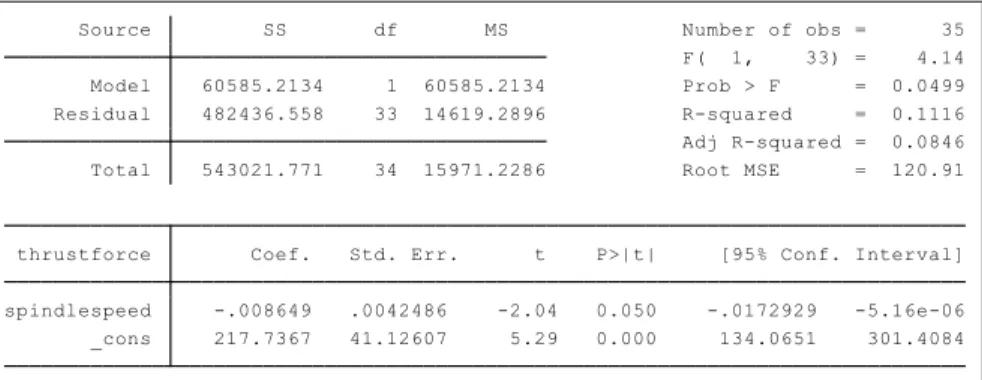
3.1 Thrust force analysis ... 27
3.1.1 Thrust force distribution study over feed rate ... 27
3.1.2 Thrust force distribution study over spindle speed ... 28
3.1.3 Thrust force multiple linear regression analysis ... 30
3.1.4 Thrust force multiple linear regression analysis with interaction ... 35
3.1.5 Thrust force data transformation... 38
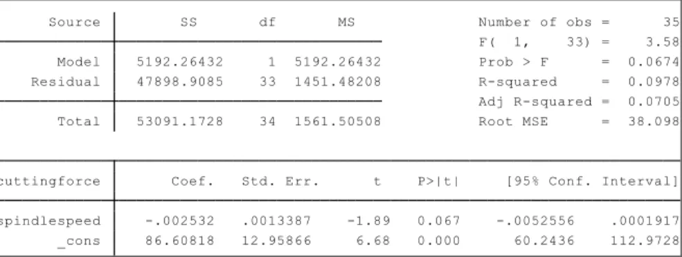
3.2 Cutting force analysis ... 42
3.2.1 Cutting force distribution study over feed rate ... 42
3.2.2 Cutting force distribution study over spindle speed ... 43
3.2.3 Cutting force multiple linear regression analysis ... 44
3.2.4 Cutting force multiple linear regression with interaction ... 48
3.2.5 Comparison of the methods used for cutting force data ... 51
3.3 Torque analysis ... 52
3.3.1 Torque distribution study over feed rate... 52
3.3.2 Torque distribution study over spindle speed ... 53
3.3.3 Torque multiple linear regression analysis ... 53
3.3.4 Torque multiple linear regression with interaction ... 57
3.3.5 Comparison of the methods used for torque... 60
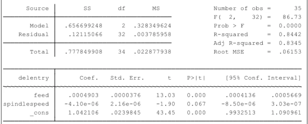
3.4 Delamination at entry analysis ... 60
3.4.1 Delamination at entry distribution study over feed rate ... 60
3.4.2 Delamination at entry distribution study over spindle speed ... 61
3.4.3 Delamination at entry multiple linear regression analysis ... 62
3.4.4 Delamination at entry multiple linear regression with interaction ... 66
3.4.5 Delamination at entry nonlinear regression ... 69
3.5 Delamination at exit analysis ... 72
3.5.1 Delamination at exit distribution study over feed rate ... 72
3.5.2 Delamination at exit distribution study over spindle speed ... 73
3.5.3 Delamination at exit multiple regression analysis ... 74
3.5.4 Delamination at exit multiple linear regression analysis with interaction ... 77
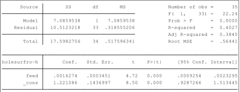
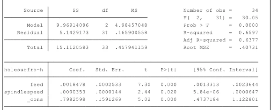
3.6 Surface roughness analysis ... 81
3.6.2 Surface roughness distribution study over spindle speed ... 82
3.6.3 Surface roughness multiple linear regression analysis ... 82
3.6.4 Surface roughness multiple linear regression analysis with interaction ... 86
3.7 Diameter error at exit analysis ... 93
3.7.1 Diameter error at exit distribution study over feed rate ... 93
3.7.2 Diameter error at exit distribution study over spindle speed ... 94
3.7.3 Diameter error at exit multiple linear regression analysis ... 95
3.7.4 Diameter error at exit transformation ... 97
3.8 Diameter error at entry analysis ... 99
3.8.1 Diameter error at entry distribution study over feed rate ... 99
3.8.2 Diameter error at entry distribution study over spindle speed ... 100
3.8.3 Hole diameter error at entry multiple linear regression analysis ... 101
3.8.4 Diameter error at entry transformation ... 103
3.9 Circularity at exit analysis... 104
3.9.1 Circularity at exit distribution study over feed rate ... 104
3.9.2 Circularity at exit distribution study over spindle speed ... 105
3.9.3 Circularity at exit multiple linear regression ... 106
3.10 Circularity at entry analysis ... 113
3.10.1 Circularity at entry distribution study over feed rate ... 113
3.10.2 Circularity at entry distribution study over spindle speed ... 114
3.10.3 Circularity at entry multiple linear regression ... 115
3.11 Delamination at exit analysis versus thrust force and cutting force ... 119
3.11.1 Delamination at exit distribution study over thrust force ... 119
3.11.2 Delamination at exit distribution study over cutting force ... 122
3.12 Delamination at entry analysis versus thrust force and cutting force ... 129
3.12.1 Delamination at entry distribution study over thrust force ... 129
3.12.2 Delamination at entry distribution study over cutting force ... 134
CHAPTER 4 CONCLUSION ... 138
LIST OF TABLES
Table 2.1: Experiment setup with 35 runs………..12
Table 2.2: Experiment setup with 18 runs...………...….12
Table 2.3: Correlation table between all variables for ANCOVA………..17
Table 3.1: The relationship between the null hypothesis and the type of statistical errors………21
Table 3.2: Controllable factors involved in the drilling process……….…23
Table 3.3: Parameter estimates and ANOVA results of thrust force against feed rate……...28
Table 3.4: Parameter estimates and ANOVA results of thrust force against spindle speed……...29
Table 3.5: Parameter estimates and ANOVA results of the thrust force using MLR……….31
Table 3.6: Shapiro-Wilk Test for thrust force normality using MLR……….33
Table 3.7: Illustration of the assumption validation results for thrust force MLR...…...35
Table 3.8: Parameter estimates and ANOVA results for thrust force using MLR-interaction…...36
Table 3.9: Shapiro-Wilk Test for Thrust Force Normality for MLR-interaction………...37
Table 3.10: Illustration of the assumption validation results………..38
Table 3.11: Goodness of fit of thrust force transformations……….………..…39
Table 3.12: Parameter estimates and ANOVA results of log-thrust force……….……39
Table 3.13: Shapiro-Wilk Test for log thrust force………40
Table 3.14: Illustration of the assumption validation results for log thrust force model………...45
Table 3.15: Comparison of all methods used for the thrust force analysis……….42
Table 3.16: Parameter estimates and ANOVA results of cutting force against feed rate………..43
Table 3.17: Parameter estimates and ANOVA results of cutting force over spindle speed……..43
Table 3.18: Parameter estimates and ANOVA results for cutting force using MLR……….44
Table 3.19: Shapiro-Wilk test for cutting force using MLR………...46
Table 3.20: Illustration of the assumption validation results for cutting force MLR……….48
Table 3.21: Parameter estimates and ANOVA results for cutting force using MLR-interaction..48
Table 3.22: Shapiro-test for cutting force using MLR-interaction……….50
Table 3.23: Illustration of the assumption validation results for cutting force using MLR- interaction...…...50
Table 3.24: Akaike’s results for Thrust force model with multiple regression–no interaction…..51
Table 3.25: Akaike’s results for Thrust force model with multiple regression–with interaction...51
Table 3.27: Parameter estimates and ANOVA results for the torque against feed rate………….52
Table 3.28: Parameter estimates and ANOVA results for the torque against spindle speed……..53
Table 3.29: Parameter estimates and ANOVA tables for the torque using MLR………..54
Table 3.30: Shapiro-Wilk test for normal data for torque using MLR………...56
Table 3.31: Illustration of the assumption validation results for torque using MLR………..57
Table 3.32: Shapiro-Wilk test for torque using MLR-interaction………..59
Table 3.33: Illustration of the assumption validation results for the torque MLR-interaction…...59
Table 3.34: Comparison of all methods used for torque analysis force analysis………60
Table 3.35: Parameter estimates and ANOVA results for the delamination at entry against feed rate……….………..…61
Table 3.36: Parameter estimates and ANOVA results for the delamination at entry against spindle speed……….………...62
Table 3.37: Parameter estimates and ANOVA results for delamination at entry using MLR……….…63
Table 3.38: Shapiro-Wilk test for normal data for delamination at entry………...65
Table 3.39: Illustration of the assumption validation results………..66
Table 3.40: Parameter estimates and ANOVA results for delamination at entry using MLR- interaction………….………...67
Table 3.41: Shapiro-Wilk test for normal data for delamination at entry………..68
Table 3.42: Illustration of the assumption validation results of delamination at entry using MLR- interaction………...…69
Table 3.43: Goodness of fit of the delamination at entry transformations………70
Table 3.44: Parameter estimates and ANOVA results of cubic transformation of the delamination at entry…….………70
Table 3.45: AIC of the squared transformation of the delamination at entry………70
Table 3.46: AIC of the MLR model of the delamination at entry………..70
Table 3.47: AIC of the MLR model with interaction of the delamination at entry………...71
Table 3.48: Critical values of the models developed for delamination at entry………71
Table 3.49: Comparison of all methods used for delamination at entry analysis………..71
Table 3.50: Parameter estimates and ANOVA results for the delamination at exit against feed rate……….………..72
Table 3.51: Parameter estimates and ANOVA results for the delamination at exit against spindle speed………73 Table 3.52: Parameter estimates and ANOVA results for delamination at exit using MLR……..74 Table 3.53: Shapiro-Wilk test for delamination at exit using MLR………...76 Table 3.54: Illustration of the assumption validation results of the delamination at exit using MLR……….………77 Table 3.55: Parameter estimates and ANOVA results for delamination at exit using MLR-
interaction………….………...78 Table 3.56: Shapiro-Wilk test for normal data for delamination at exit………79 Table 3.57: Illustration of the assumption validation results for delamination at exit MLR-
interaction……….…..……….80 Table 3.58: Goodness of fit of the delamination at exit transformations………..………….80 Table 3.59: AIC of the MLR model of the delamination at exit……….…...80 Table 3.60: AIC of the MLR model with interaction of the delamination at exit………..………80 Table 3.61: Comparison of all methods used for delamination at exit analysis………….………80 Table 3.62: Parameter estimates and ANOVA results of the surface roughness over feed rate….81 Table 3.63: Parameter estimates and ANOVA results of the surface roughness over spindle
speed……….………...82 Table 3.64: Parameter estimates and ANOVA results for surface roughness using MLR……….83 Table 3.65: Shapiro-Wilk test for normal data for surface roughness………85 Table 3.66: Illustration of the assumption validation results for the surface roughness using MLR……….………86 Table 3.67: Parameter estimates and ANOVA results for surface roughness using MLR-
interaction……….………...87 Table 3.68: Shapiro-Wilk test for surface roughness using MLR-interaction……..………..88 Table 3.69: Illustration of the assumption validation results for surface roughness with MLR- interaction……….……….…..89 Table 3.70: Outlier in surface roughness transformation……….………..89 Table 3.71: DFBETA of feed rate and spindle speed in surface roughness transformation……..89 Table 3.72: Parameter estimates and ANOVA results for the surface roughness with n=34….…90 Table 3.73: Shapiro-Wilk Test for surface roughness with n=34………..….91
Table 3.74: Akaike’s results for surface roughness model with MLR-interaction………...……..92 Table 3.75: Akaike’s results for surface roughness model with MLR n=34…………..…………92 Table 3.76: Comparison of all methods used for surface roughness…………..………93 Table 3.77: Parameter estimates and ANOVA results for the diameter error at exit against feed rate……….……….……….94 Table 3.78: Parameter estimates and ANOVA results for the diameter error at exit against spindle speed………...……….……95 Table 3.79: Parameter estimates and ANOVA results for diameter error at exit using MLR…....96 Table 3.80: Testing results of the transformations of the diameter error at exit………..…...97 Table 3.81: Test of the transformation of the feed rate………...98 Table 3.82: Parameter estimates and ANOVA results for diameter error at exit…………..…….98 Table 3.83: Comparison of all methods used for the diameter error at exit………...99 Table 3.84: Parameter estimates and ANOVA results for diameter error at entry against feed rate……….…100 Table 3.85: Parameter estimates and ANOVA results for diameter error at entry against spindle speed……….……….101 Table 3.86: ANOVA and parameter estimates tables for the diameter error at entry using
MLR……….….……….102 Table 3.87: Results for the transformation of the diameter error at entry………103 Table 3.88: BFBETAs for diameter error at entry………104 Table 3.89: Comparison of all methods used for the diameter error at entry analysis………….104 Table 3.90: Parameter estimates and ANOVA results for circularity at exit against feed rate…105 Table 3.91: Parameter estimates and ANOVA results for circularity at exit against spindle
speed…...106 Table 3.92: Parameter estimates and ANOVA results for the diameter error at exit MLR…….106 Table 3.93: Shapiro-Wilk test for normal data of the circularity at exit data using MLR………108 Table 3.94: Illustration of the assumption validation results for circularity at exit using MLR..109 Table 3.95: Values of DFBETA of feed rate and spindle speed for circularity at exit………….110 Table 3.96: Parameter estimates and ANOVA results for hole circularity at exit with n=34…..111 Table 3.97: Akaike’s results for circularity at exit model with MLR………...…112 Table 3.98: Akaike’s results for circularity at exit model with multiple regression–n=34…...112
Table 3.99: Comparison of all methods used for the circularity at exit analysis………..113 Table 3.100: Parameter estimates and ANOVA results for circularity at entry over feed rate…114 Table 3.101: Parameter estimates and ANOVA results for circularity at entry over spindle
speed………...……….115 Table 3.102: Parameter estimates and ANOVA results for circularity at entry using MLR…....115 Table 3.103: Shapiro-Wilk test for the circularity at entry………...117 Table 3.104: Illustration of the assumption validation results for circularity at exit………118 Table 3.105: Comparison of all methods used for the circularity at entry analysis……….118 Table 3.106: Parameter estimates and ANOVA results of delamination at exit against thrust force………...………..119 Table 3.107: Shapiro-Wilk Test for delamination at exit normality delamination at exit against thrust force………...………120 Table 3.108: Illustration of the assumption validation results for delamination at exit-simple regression………...…..121 Table 3.109: Parameter estimates and ANOVA results of cutting force against delamination at exit………..……….122 Table 3.110: Shapiro-Wilk Test for cutting force normality using simple regression………….123 Table 3.111: Illustration of the assumption validation results for delamination at exit versus cutting force using simple regression………..124 Table 3.112: Parameter estimates and ANOVA results of delamination at exit against cutting force using nonlinear regression………..……...125 Table 3.113: Parameter estimates and ANOVA results of thrust force and cutting force against delamination at exit………..………...126 Table 3.114: Shapiro-Wilk Test for delamination at exit normality using MLR……….127 Table 3.115: Parameter estimates and ANOVA results of delamination at entry against thrust force………...………..129 Table 3.116: Shapiro-Wilk Test for delamination at entry normality using simple regression…130 Table 3.117: Illustration of the assumption validation results for delamination at entry with
simple regression……….131 Table 3.118: Parameter estimates and ANOVA results of transformed thrust force against
Table 3.119: Shapiro-Wilk test for normal data for delamination at entry………...133
Table 3.120: Illustration of the assumption validation results………..134
Table 3.121: Parameter estimates and ANOVA results of cutting force against delamination at entry………...………..134
Table 3.122: Shapiro-Wilk Test for cutting force normality using simple regression……….…135
Table 3.123: Illustration of the assumption validation results for delamination at entry vs cutting force using simple regression………..136
Table 3.124: Presentation of all analysis completed for the delamination at entry against thrust force and cutting force………..……….….………….137
Table 4.1: Coded values for the feed rate and spindle seed settings…….……….. 139
Table 4.2: Relationship between independent variables and outputs……….………..139
LIST OF FIGURES
Figure 1.1: Representation of the delamination factor and mechanism ……..………3
Figure 1.2: Surface Roughness illustration………...3
Figure 1.3: Representation of the hole circularity errors………..4
Figure 1.4: Representation of the hole diameter error………..4
Figure 1.5: Two Flute Standard Point Solid Carbide Twist Drill of 5 mm diameter ………..6
Figure 1.6: Makino A88………....6
Figure 2.1: The basic geometric representation for a box-behnken design for three factors…….10
Figure 3.1: Thrust force boxplot against feed rate………..28
Figure 3.2: Thrust force boxplot against spindle speed………..29
Figure 3.3: Thrust force plot fitted against observed values using MLR………...32
Figure 3.4: Plot of residuals of the thrust force data versus run order………32
Figure 3.5: Normal probability plot for the thrust force data using MLR………..33
Figure 3.6: Residual plot for the thrust force data using multiple regression……….34
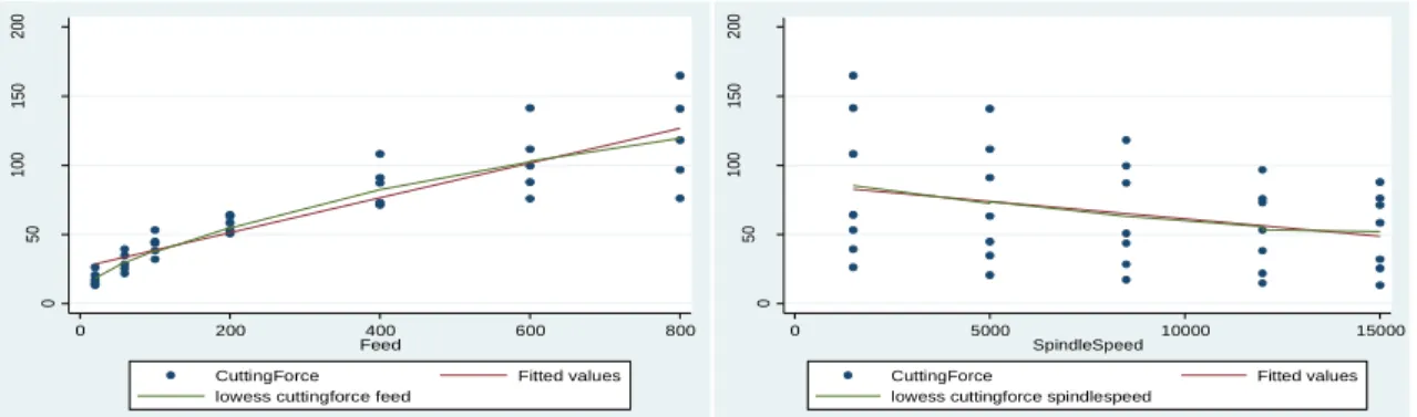
Figure 3.7: Scatterplots of thrust force versus feed rate and spindle speed………34
Figure 3.8: Thrust force plot fitted against observed values using MLR-interaction………36
Figure 3.9: Normal probability plot of standardized residuals for the thrust force with MLR- interaction………..………...37
Figure 3.10: Thrust force fitted values against standardized residuals………..38
Figure 3.11: Plot of the log thrust force fitted model against the feed rate and spindle speed…..40
Figure 3.12: Plot of residual vs fitted values for log thrust force transformation………..41
Figure 3.13: Scatterplot of feed rate and spindle speed against log thrust force………41
Figure 3.14: Boxplot of feed rate against cutting force………..42
Figure 3.15: Boxplot of cutting force against spindle speed………..44
Figure 3.16: Plot of the observed vs predicted values for cutting force using MLR……….45
Figure 3.17: Plot of standardized residuals of the cutting force versus case number………45
Figure 3.18: Normality plot of the standardized residuals of the cutting force data………..46
Figure 3.19: Cutting force fitted values versus residuals………47
Figure 3.20: Scatterplots feed rate and spindle speed against cutting force………...47
Figure 3.21: Observed vs predicted values of the cutting force using MLR-interaction…………49
Figure 3.23: Plot of fitted against residual values for cutting force with MLR-interaction…..….50
Figure 3.24: Boxplot of the torque against the feed rate………52
Figure 3.25: Boxplot of the torque against the spindle speed………53
Figure 3.26: Plot of observed versus predicted values for torque using MLR……….…………..55
Figure 3.27: Plot of the standardized residuals of the fitted torque against the run order of the data collection……….…………55
Figure 3.28: Normality plot for the torque experimental data………56
Figure 3.29: Observed vs residual values plot of the torque data using MLR………...56
Figure 3.30: Scatterplots feed rate and spindle speed against torque……….57
Figure 3.31: Plot of torque observed against predicted values using MLR-interaction………….58
Figure 3.32: Normal probability plot of the torque using the MLR-interaction……….59
Figure 3.33: Predicted torque values against residuals using MLR-interaction……….59
Figure 3.34: Boxplot of delamination at entry against feed rate………61
Figure 3.35: Boxplot of delamination at entry against spindle speed………62
Figure 3.36: Delamination at entry observed values against predicted using MLR………..64
Figure 3.37: Plot of the standardized residuals of the fitted delamination at entry against the run order of the data collection………...…..64
Figure 3.38: Normality plot for the delamination at entry………..65
Figure 3.39: Predicted vs standardized residual values plot of the delamination at entry………..65
Figure 3.40: Scatterplots feed rate and spindle speed vs delamination at entry……….…66
Figure 3.41: Delamination at entry observed against predicted values using MLR- interaction………...67
Figure 3.42: Normality plot for delamination at entry using MLR-interaction……….…………68
Figure 3.43: Residual plot versus fitted data of delamination at entry using MLR-interaction….68 Figure 3.44: Boxplot of delamination at exit against feed rate………..72
Figure 3.45: Boxplot of delamination at exit against spindle speed………..74
Figure 3.46: Delamination at exit estimated plot using MLR………75
Figure 3.47: Plot of the standardized residuals of the fitted Delamination at exit against the run order of the data collection……….75
Figure 3.48: Normality plot for the delamination at exit with MLR………..76
Figure 3.50: Scatterplot feed rate and spindle speed vs delamination at exit……….77
Figure 3.51: Predicted vs standardized residual values plot of the delamination at exit experimental data………78
Figure 3.52: Normality plot for the delamination at exit with MLR-interaction………79
Figure 3.53: Predicted vs standardized residual values plot of the delamination at exit using MLR-interaction……….79
Figure 3.54: Boxplot of surface roughness against feed rate………..81
Figure 3.55: Boxplot of surface roughness against spindle speed………..82
Figure 3.56: Surface roughness observed values against predicted using MLR………84
Figure 3.57: Plot of the standardized residuals of the fitted surface roughness against the run order of the data collection……….84
Figure 3.58: Normality plot for the surface roughness experimental data……….85
Figure 3.59: Predicted vs standardized residual values plot of the delamination at exit…………85
Figure 3.60: Scatterplots feed rate and spindle speed vs hole surface roughness………..86
Figure 3.61: Surface roughness observed values against predicted using MLR-interaction…….87
Figure 3.62: Normality plot of the surface roughness data using MLR-interaction………..88
Figure 3.63: Predicted vs standardized residual values plot of the surface roughness using MLR- interaction………...………88
Figure 3.64: Surface roughness observed values against predicted using MLR with n=34...……90
Figure 3.65: Plot of normality of the surface roughness with n=34………...91
Figure 3.66: Residual plot of the surface roughness experimental data with n=34………92
Figure 3.67: Boxplot of diameter error at exit against feed rate……….93
Figure 3.68: Boxplot of diameter error at exit against spindle speed……….94
Figure 3.69: Predicted vs standardized residual values plot of the diameter error at exit……….97
Figure 3.70: Residual plot for the diameter error at exit experimental data………..99
Figure 3.71: Diameter error at entry boxplot against the feed rate………...100
Figure 3.72: Diameter error at entry boxplot with the spindle speed………...101
Figure 3.73: Residual plot for diameter error at entry using MLR………...…103
Figure 3.74: Boxplot of the circularity at exit over feed rate………...…104
Figure 3.75: Boxplot of the circularity at exit over spindle speed………105
Figure 3.77: Plot of the standardized residuals of the circularity at exit data against the number of
cases……….….107
Figure 3.78: Normal plot of the standardized residuals of the circularity at exit data…………..108
Figure 3.79: Residuals plot for circularity at exit……….108
Figure 3.80: Scatterplots feed rate and spindle speed against circularity at exit………..…109
Figure 3.81: Plot of the leverage against normalized residual squared of the circularity at exit………....109
Figure 3.82: Plot of the circularity at exit fitted vs observed values n=34……..……….…112
Figure 3.83: Boxplot of circularity at entry over the feed rate……….113
Figure 3.84: Boxplot of circularity at entry over the spindle speed……….…114
Figure 3.85: Plot of the circularity at entry fitted vs observed values using MLR………...116
Figure 3.86: Plot of standardized residuals of the circularity at entry against case number…...116
Figure 3.87: Plot of standardized residuals of the circularity at entry……….……….117
Figure 3.88: Scatterplots feed rate and spindle speed against circularity at entry………117
Figure 3.89: Residuals plot for circularity error at entry………..……118
Figure 3.90: Plot of the thrust force against the delamination at exit………...…120
Figure 3.91: Normal probability plot for the delamination at exit simple regression………..…120
Figure 3.92: Residual plot for the delamination at exit data using simple regression…………..122
Figure 3.93: Scatterplot of thrust force versus feed rate………...122
Figure 3.94: Plot of the cutting force against the delamination at exit……….…123
Figure 3.95: Normal probability plot for the cutting force data against the cutting force………123
Figure 3.96: Residual plot for the cutting force versus delamination at exit data using simple linear regression………...………...….124
Figure 3.97: Scatterplot of cutting force against delamination at exit………..124
Figure 3.98: Plot of the quadratic delamination at exit fitted model………126
Figure 3.99: Plot of the delamination at exit using MLR……….127
Figure 3.100: Normal probability plot for the delamination at exit using MLR………..…127
Figure 3.101: Normal probability plot for the delamination at exit using MLR……….….127
Figure 3.102: Residual plot for the delamination at exit data using MLR……….…..128
Figure 3.103: Test of collinearity……….……128
Figure 3.105: Normal probability plot for the delamination at entry using simple regression with thrust force………..………....130 Figure 3.106: Plot of the delamination at entry observed vs predicted values against thrust force transformation………..………...132 Figure 3.107: Normal plot of the standardized residuals of the delamination at entry……..…...133 Figure 3.108: Scatterplot of the delamination at entry against the log (thrust force)…….……..133 Figure 3.109: Residuals plot for circularity at exit………...134 Figure 3.110: Plot of the cutting force against the delamination at entry….………135 Figure 3.111: Normal probability plot for the delamination at entry vs cutting force data using simple regression………..……..135 Figure 3.112: Residual plot for the delamination at entry versus cutting force data using simple regression………..………..136 Figure 3.113: Scatterplot of cutting force against delamination at entry………..136
LIST OF ABBREVIATIONS
MLR Multiple Linear RegressionANOVA Analysis of variance RSM Response Surface Model
NRC National Research Council of Canada CFRP Carbon Fiber Reinforced Polymer BBD Box-Behnken Design
ANN Artificial neural network SVR Support Vector Regression
FP False Positive
FN False Negative
SRM Structural Risk Minimization SVM Support Vector Machines
R2adj Adjusted coefficient of determination
Ln Logarithmic scale
ANCOVA Analysis of covariance
Tf Thrust force
Cf Cutting force
T Torque
Den Delamination at entry Dex Delamination at exit
SR Surface Roughness
Drx Diameter Error at Exit Dre Diameter Error at Entry Cex Circularity at Exit Cen Circularity at Entry dmax Maximum diameter
d Hole diameter
SS Sum Square
df Degrees of Freedom
AIC Akaike Information criterion BPCW Breusch-Pagan/Cook-Weisberg
LIST OF ANNEXES
ANNEX A.….……….………..…146 ANNEX B.………....147 ANNEX C...………...…149
CHAPTER 1 INTRODUCTION
Over the years, composites were found to be one of the most important materials used in many critical industries: infrastructure, aerospace, and military applications because of its several structural advantages and qualities: rigidity, durability, lightness, corrosion resistance and hardness. That being said, the cost remains relatively high. Composites are products made from two major constituents: fiber and matrix whereas the matrix provides protection of the fiber. This combination provides the final product built with the composites material higher and surpassing performance than the starting materials. The structural behavior depends on the properties of the fibers (their amount and orientations) and the matrix, and is manufactured in distinct layers. These different layers or plies bonded together form a laminate [1].
The fabrication methods in these different industries range from very simple to complex processes with expensive operations equipment. Machining of composites materials is one of the critical processes. The most common machining processes are drilling, turning, cutting and milling. The process selected to fabricate the end product using the composite part is dependent upon factors such as the design requirements, part complexity and surface finish and appearance. The manufacturing method analyzed in this research is drilling.
Drilling is the most popular conventional machining process and one of the most essential metal-cutting operations, comprising approximately 33% [2] of all metal-metal-cutting operations. The drilling process is mainly characterized by the feed rate, the cutting speed, the tool (coated/uncoated), the laminate design and the cooling strategy. These factors are known to be controllable because they are defined by the process experts and can be regulated by the operator. Also, other uncontrollable factors, which can only be measured during the running of the process, are involved. These factors are the thrust force, the torque, the cutting force, the cutting temperature, and the tool wear. At the process monitor and control level, most of the hole’s defects observed are surface delamination, circularity errors, surface roughness and diameter error. These undesirable imperfections need to be investigated to avoid the failure of the material structure. In an aircraft construction for example, the holes must be drilled with keen attention to ensure minimum defects based on pre-defined design and manufacturing requirements, and error tolerance. Failure to do so can result in the parts becoming scrapped and major disaster of the whole product dysfunction. This study addresses the problems related to the characterizations
presented above to develop an approach for damage-free drilling composites by predicting their comportment.
A. Organization of the dissertation
Feed rate and spindle speed are the only two parameters considered in this study as the controllable and explanatory variables. Accordingly, in chapter 1, the quality characteristics of the delamination at entry, the delamination at exit, the hole surface roughness (in microns), the hole diameter error at exit (in %), the hole diameter error at entry (in %), the hole circularity at exit (in %) and the hole circularity at entry (in %) are explained to understand their effect on the drilling process performance. Also, the uncontrollable variables (thrust force, cutting force and torque) impacts are explored.
In chapter 2, a literature review of past studies, facts and experiments are presented to identify the researcher’s methodologies and works in modeling drilling operation.
In chapter 3, analytical models of the uncontrollable variables and the quality characteristics are developed using the regression method. A detailed presentation and analysis of this technique are underlined. As a result, the accuracy of each model will be investigated for future usage.
B. Statement of the problem and process parameters
During this drilling process, seven hole quality characteristics outputs are measured: the delamination at entry, the delamination at exit, the surface roughness, the diameter error at exit, the diameter error at entry, the circularity at exit and the circularity at entry. Their definition and impact is presented below.
The delamination is one of the major concerns in drilling. It is considered a severe damage since it reduces the service life of the material. It is caused by the acting between the drill feed motion and the thrust force that leads to cracks between the plies in the drilled hole which may result in deterioration of its mechanical performance (durability and strength). The surface delamination is defined by the separation of the plies where the cutter enters and exits the composite materials. Therefore, two types of delamination are differentiated: the push-out at entry and the peel-up at exit. Figure 1.1 displays a representation of the delamination factor and its mechanism.
Figure 1.1: Representation of the delamination factor and mechanism [3]
The delamination is mostly affected by the feed rate, spindle speed, drill diameter, drill point design, and material configuration [3]. The delamination on the outer surface plies generally increases with the rise of the feed rate and spindle speed. Also, it is noticed that the exit delamination is highly correlated with the thrust force which is dependent on the drill point geometry [3]; the push-out delamination is reduced by lowering the thrust force. Also, it has been found that the push-out delamination is more severe than the peel-up [4]. The delamination could be measured by different practices: digital image processing [5], ultrasound [6], x-ray [7], and laser-based imaging [8]. In machinability, an improved delamination is obtained by machining at high spindle speeds and low feed rates. A delamination factor (F) is defined as the ratio of the maximum diameter (dmax) of the damage zone to the hole diameter (d) [4]: 𝐹 =
𝑑𝑚𝑎𝑥
𝑑 .
Another essential quality characteristic to be precisely controlled and monitored by the experts is the surface roughness which corresponds to the finer surface irregularities on the surface’s texture. Figure 1.2 illustrates the surface roughness as a result of the manufacturing process [8]. Surface finish in drilling composite materials have been found to be influenced by the feed rate, cutting speed, drill geometry, tool wear and tool material [9].
Another important quality attribute in drilling is the circularity; it is measured at entry and exit. A large circularity value is problematic for parts with relative motion because it induces vibration and heat. Figure 1.3 represents a sketch of the circularity error. The circularity of the microhole essentially reflects the surface finish at the rim of the hole machined and is measured from the difference between two concentric boundaries: maximum and minimum height of the irregularities at the rim [11].
Figure 1.3: Representation of the hole circularity errors [11]
An additional output of interest for the hole quality is the diameter error; it is measured at entry and exit using a coordinate measuring machine. In drilling, it is important to produce accurate diameter within pre-defined tolerances. The difference between the measured diameter and the designed diameter is the diameter error. As a result, a positive error indicates over-sizing of the holes. Figure 1.4 illustrates the diameter error.
Figure 1.4: Representation of the hole diameter error [12]
During this drilling process, three uncontrollable variables (thrust force, cutting force and torque) are measured to study their behavior when varying the feed rate and the spindle speed at different levels. The definition and the main interests of these variables are presented below.
The thrust force is generated by the cutting action of the cutting edges and the chisel edge. For metal, using conventional twist drill, the thrust force could be correlated with the feed rate and the drill diameter by the empirical relationship below [4].
𝐹𝐴 = 𝑑2𝐻𝐵[ 𝐾1 𝑓0.8 𝑑1.2+ 𝐾2( 𝑐 𝑑)2 ] Where:
HB is the work piece Brinell hardness in kg/mm2
f is the feed rate in mm/rev c is the chisel edge length
K1 and K2 are constants that depend on the work piece material, thickness and
drill point geometry
The torque is caused by the cutting force couple (Fc) acting on the major cutting edges and its magnitude is defined by the magnitude of the cutting force and the drill diameter (d) [4]. Mathematically, the torque is represented by: 𝑀 = 𝐹𝑐𝑑2.
The force and torque signals were measured using a Kistler-four component piezoelectric dynamometer model 9272. The thrust force and the torque are influenced by the feed rate, the cutting speed and the drill geometry. They both increase significantly with the rise of the feed rate due to its direct influence on uncut chip size. Also, it has been observed that the interaction combining the effect of the feed rate and the drill diameter on the thrust force and the torque is found to be more significant than the separate effect of either one of the variables. However, the cutting speed effect could have less significant effect on the thrust force and the torque [4]. The cutting force is dependent on the feed rate, and it is generally directly proportional to it [4]. In this experiment, the cutting force was derived from the torque.
Therefore, a big challenge is facing the industry of drilling manufacturing: how can they produce higher quality holes with minimum damages. To understand the effects and relations between the factors under study and the quality characteristics while drilling a composite material, several studies are conducted using the following statistical methods: multiple linear regression (MLR), analysis of variance (ANOVA) and response surface model (RSM).
C. Description of the tool
The tool material used in the present investigation is a standard carbide twist drill (M43236), a product of Kennametal Inc. This drill is a 2- flute, right hand spiral, right-hand cut drill with a 30o helix angle and 118o point angle. The carbide grade is ISO K10 - K20 with approximately 7% cobalt as binder. This drill is shown in Figure 1.5.
Figure 1.5: Two Flute Standard Point Solid Carbide Twist Drill of 5 mm diameter
D. Description of the machine
The drilling experiments were carried out on a 5-axis high-speed, high-power horizontal machining centre Makino A88 (shown in Figure 1.6). It has the following characteristics: 50 kW spindle power, 3 linear and 2 rotary axes, maximum spindle speed of 18,000 rpm, maximum feed rate of 50 m/min, minimum feed setting unit of 1µm, tool clamping force of 19.6 kN and HSK 100A spindle adapter.
Figure 1.6: Makino A88
E. Description of the material
The work piece comprised of woven carbon fibre as the reinforcements and epoxy as the matrix material. The woven prepreg, L-930 HT 139, used for manufacturing the laminate was supplied by J.D. Lincoln Inc. The woven prepreg was a plain weave fabricated out of T300 graphite fibers each having 3000 filaments.
F. Research objectives
The objective of this research is to formulate analytical models to predict the quality characteristics under study and the uncontrollable variables during the drilling of composite material using the regression method.
Therefore, the following steps will be used:
a) Use a full factorial design with two factors at appropriate levels of the independent variables.
b) Analyze the data distribution of each output to understand the existing relationship with the input variables.
c) Develop a mathematical model of each output using the multiple linear regression method.
d) Add an interaction effect of the independent variables to the model and refit the data to a new multiple linear regression model.
e) If an accurate model couldn’t be found through the multiple regression methodology, attempt a new fitting with the nonlinear regression technique or different types of transformation.
f) For each developed model, check the model adequacy by demonstrating how well the model fits the observed data and how well the regression model predicts new observations.
CHAPTER 2 LITERATURE REVIEW
In the literature, several experiments were carried out on drilling of CFRP composites. S. Jayabal & U (2010) used a full factorial design with three factors at three levels each (33 equal 27 experimental runs) to evaluate the mechanical and machinability characteristics of hybrid composites [13]. The measured responses were the thrust force, the torque and the tool wear and the process control factors were the bit-drill diameter, the spindle speed and the feed rate. The multiple regression technique was used to identify the mathematical model of the interaction of the specified main effects in the drilling process. The machinability study determined that the feed rate has the most significant role on the machining characteristics. To conclude their experiment, the authors defined the best combination of the drilling parameters to minimize the effects of the thrust force, the torque and the tool wear. Using this design, the average absolute errors for thrust force (2.56%), torque (2.91%) and tool wear (2.93%) are between 2.5% and 3%. The variability of the model was 92.96% for thrust force, 89.32% for the torque and 96.72% for the tool wear which is considered very good estimates.
In another paper, S. Jayabal & U. Natarajan (2011) carried out a statistical modeling to develop mathematical models to relate few outputs (thrust force, torque and tool wear) to three inputs (drill-bit diameter, feed rate and spindle speed) through the multiple linear regression technique [14]. The ANOVA was performed to test the significance of the obtained coefficients at one per cent level of significance. The developed models were verified by eight sets of experiments. They used a Box-Behnken Design (BBD) with three factors at three levels each to study the effects of each factor and their interactions on predefined hole’s characteristics with a total of 17 experiments. To analyze the collected data, a quadratic design was chosen for the thrust force and the torque models. However, linear terms were used to define the model of the tool wear. The RSM was used to define the optimal responses (thrust force, torque and tool wear) for each input (drill bit diameter, spindle speed and feed rate). In that study, the feed rate and the drill bit diameter were found to be the most significant factors affecting the thrust force. To confirm the accuracy of the obtained results, the percentage of the error between the observed and predicted values was calculated using the following equation:
% of error = 𝑝𝑟𝑒𝑑𝑖𝑐𝑡𝑒𝑑 𝑣𝑎𝑙𝑢𝑒 − 𝑒𝑥𝑝𝑒𝑟𝑖𝑚𝑒𝑛𝑡𝑎𝑙 𝑣𝑎𝑙𝑢𝑒 𝑝𝑟𝑒𝑑𝑖𝑐𝑡𝑒𝑑 𝑣𝑎𝑙𝑢𝑒
Using the developed mathematical model, the percentage of error calculated was within the acceptable ranges which confirm the adequacy of the results. In fact, the average absolute errors for the thrust force (0.4%), the torque (0.08%) and the tool wear (0.57%) were less than 1%. The variability of the model was 99.88% for the thrust force, 99.88% for the torque and 96.22% for the tool wear.
The difference between the previous two papers presented above is that the authors chose to use a full experiment design in the first versus a BBD in the second. In general, every machine used in a production process allows its operators to adjust various settings affecting the quality characteristics of the manufactured product. Experimentation and testing allow the manufacturing engineer to learn which factors have the highest impact on the resultant quality characteristics by adjusting the settings of the machine in a methodical manner. Using this information, the settings can be regularly enhanced until optimum features are achieved. Moreover, it is important to know what to change in order to produce a better product at minimum cost. At first, experimenters considered three factors (bit-drill diameter, spindle speed and feed rate) affecting the production process at three levels to determine whether any of these changes would affect the outputs under study (thrust force, torque and tool wear). The most instinctive approach to study those factors would be to vary the three factors (thrust force, torque and tool wear) in a full factorial design; to try all possible combinations of settings. This method is acceptable when the number of factors under study and the settings are small. In fact, the number of necessary observations (runs in the experiment) increases when more factors and settings are involved. For example, to study six factors, the necessary number of runs in the experiment would be 26 = 64 observations and for 10 factors, it’s 210 = 1024 observations. Every observation involves time and cost to set and reset the machine. In a production environment, it’s usually not feasible to run a high volume of a set of production for the experiment. In these conditions, fractional factorials (reduced number of observations) are used to "sacrifice" interaction effects so that the main effects may still be computed correctly. By running fewer experiments, the same results and conclusions may be pulled to determine the optimum values of the process and to analyze the behavior of each factor. In the second paper, the authors selected an alternate design of experiment to reveal significant interactions and find the optimum operating conditions for a high-quality drilling: the BBD. This design is specially made for factors with three levels coded as (-1, 0, +1). BBD is an independent
quadratic design and not a fractional factorial design. Consequently, with the same 3 factors (bit-drill diameter, spindle speed and feed rate), 17 runs are completed:
Four points in the center of each face which makes a total of 12 points (refer to figure 2.1 for a basic illustration), and
Five replicates of the center points.
Figure 2.1: The basic geometric representation [15] for a BBD for three factors
The use of +1 and -1 for the variable settings is called “coding the data”. In this case, the authors used three coded levels: -1 for the higher value, 0 for the center point and +1 for the lower value. This specific methodology was chosen to fit a second-order response surfaces for the three factors under study. In both papers, the results are showing that the most important factor affecting the thrust force, torque and tool wear is the feed rate. In fact, the BBD methodology compared to the full factorial experimental design saved the researchers 10 experiments; a significant difference in time, material consumption and cost. The lesson to learn is that BBD can efficiently be applied for modeling drilling factors (bit-drill diameter, spindle speed and feed rate) in an economical way of obtaining the information with least number of runs. Refer to annex B note 5 for the experimental design matrix in terms of coded factor levels for a BBD for three factors.
Coding is a simple linear transformation of the original measurement scale. In the real scale, the highest value is Xh and lowest is XL. The scaling transformation takes any original X value and
converts it to: 𝑇𝑅(𝑋) = (𝑋 − 𝐴) 𝐵 Where: 𝐴 = 𝑋ℎ+𝑋𝐿 2 ; 𝐵 = 𝑋ℎ−𝑋𝐿 2
If X = Xh then, TR(Xh)= (Xh-XL)/ (Xh-XL) = 1. If X = XL then, TR(XL)= - (Xh-XL)/ (Xh-XL) = -1.
If X = average of the settings = A then, TR(Xavg)=[(Xh+XL)-(Xh+XL)]/(Xh-XL)= 0.
To transform back a coded value to its original measurement scale, multiply the coded value by B then, add A: 𝑋 = (𝑐𝑜𝑑𝑒𝑑 𝑣𝑎𝑙𝑢𝑒) ∗ 𝐵 + 𝐴. As an example, if the variable X is pressure and the high setting is 100 psi and the low setting is 20 psi then, A= (100 + 20)/2 = 60 psi and B = (100 - 20)/2 = 40 psi. The real value of the coded value of the center point 0 has a temperature of: X = 0*(40) + 60 = 60 psi.
Before presenting further studies, the design of experiments (DOE) concept is explained. The DOE screens a large number of factors with a minimum sample size. From a cost-effective and time-reduction point of view, engineers and physicists can no longer afford to experiment in a trial-and-error manner testing by changing one factor at a time. Consequently, a more effective method known by design of experiments, has been conceived. It’s an efficient systematic approach and powerful tool based on a stochastic search technique for solving optimization problems, which has been widely applied in many scientific and engineering fields for process efficiency and product quality. The type of design is highly dependent on the number of factors studied. This method:
Considers all factors simultaneously;
Provides an effective way to solve serious operational and production problems; and
Reveals information about the interaction of factors and the way the whole system works (even the interaction between the factors), a fact not obtainable through testing one factor at a time.
The input factors are independent variables that affect the responses and outputs under study. Each factor has a set of settings defined by the experimenter. This approach tackles the drilling quality problems by performing the minimum number of experiments needed. Then, develop analytical equations that express all the important and significant factors which can be used, depending on the drilling conditions to predict the desired outputs. Therefore, the constructed model is able to identify the significant factors affecting one or multiple outputs, achieve an optimal process output (combination for best quality) and reduce variability. Refer to annex A to understand in details how to build a DOE.
In this research, the experts completed 35 runs which are considered a full factorial plan that combines all combinations with no replications. Other plans can be built to provide more adequate results. Here are two recommended designs that can be used:
With the same number of runs: 22+1 with 7 replicates equal to 35 runs. In this case, two levels (minimum and maximum) are defined for each input variables: feed rate (20, 800) and spindle speed (1500, 15000). The “+1” represents the center point (200, 8500). In this design, the observations in table 2.1 are replicated 7 times.
Table 2.1: Experiment setup with 35 runs Run # Feed rate Spindle speed
1 20 1500
2 20 15000
3 800 1500
4 800 15000
5 200 8500
With less number of runs: 23 with two replications equal to 18 runs. In this case, three levels (minimum, center and maximum) are defined for each input variables: feed rate (20, 200 and 800) and spindle speed (1500, 8500 and 15000). This design represents half of the current experiments done and will provide good results. In this design, the observations in table 2.2 are replicated twice.
Table 2.2: Experiment setup with 18 runs Run # Feed rate Spindle speed
1 20 1500 2 20 8500 3 20 15000 4 200 1500 5 200 8500 6 200 15000 7 800 1500 8 800 8500 9 800 15000
Replications are added in both plans to determine the experimental error εi.
In another study, the authors [16] performed an analysis of the thrust force in drilling of glass fiber-reinforced plastic. During this investigation, the spindle speed, the feed rate, and the drill diameter were considered as machining input parameters at three levels each. The authors
selected “Tagushi’s L27” experimental design with three repetitions (81 runs in total) to examine
the relations between the inputs (spindle speed, feed rate, and drill diameter) and the output (thrust force). For a first estimation, Pareto ANOVA (a graphical method to understand the overall relationships but not very exact whereas no error terms are considered) was employed to determine the significant factors and interactions. For further analysis, the ANOVA was exploited at 95% confidence level to understand the effects of every factor. Using the RSM, a mathematical model was deduced and the correlation verified between the spindle speed, feed rate, and drill diameter, and the thrust force. As per the authors, the obtained results are only near optimal. As reported in many papers, to analyze the process and to find the optimum response, one may turn to the RSM methodology. The RSM is the collection of mathematical and statistical techniques that are useful for the modeling and analysis of problems in which a response of interest is influenced by several variables and the objective is to optimize that response [18]. RSM also quantifies the relationship between the controllable input parameters and the obtained response surfaces [19]. This technique helps experts to define the best settings combination for the factors under study to provide the most appropriate values for the desired responses.
An alternative approach [17] involving the design of experiments has been used to select the optimal cutting parameters of carbon fiber reinforced thermosets. The input variables under study were cutting speed, feed rate and tool point angle at five levels each. The outputs to be optimized for enhanced hole quality characteristics are the thrust force, the delamination, the damage width and the surface roughness. The methodology used in that study combines tagushi’s technique, RSM and ANOVA.
Another related research involves the use of the regression technique is presented. In this paper [20], the authors employed regression and artificial neural network (ANN) to predict tool wear in end milling. The conducted experiments to measure tool wear are based on the DOE of five levels of four factors full factorial technique. The input variables under study are the feed rate, the helix angle, the spindle speed and the depth of cut against the tool wear being the only output. The ANN techniques provided a higher accuracy rate (average error < 2%) models compared to the results obtained from the classic statistical regression model (average error < 5%). As a first step, the authors normalized all the raw data of input values to develop an appropriate model via the regression model. Then, they used the data generated from the previous model to demonstrate a
new one through the ANN method to predict the minimum value of tool wear and estimate the best combination values of the process.
During this exploration, some researchers used the ANN and the support vector regression (SVR) methods to predict the drilling and cutting output values for better sensitivity and specificity; statistical measures of the performance of the diagnostic. The sensitivity is the capability to correctly identify the output with the identified problem; however test specificity is to incorrectly identify those with the known problem. There are two types of errors intrinsic in every technique [21]:
Sensitivity = error Type I (FP - False Positive): error of deciding when an action should be taken while the system is in a normal condition and,
Specificity = error Type II (FN - False Negative): error of deciding that the system is in a normal condition while it is not.
There are four possible outcomes of the simulation:
True negative (a) = correctly rejected
False negative (b) = incorrectly rejected
False positive (c) = incorrectly identified
True positive (d) = correctly identified
From a mathematical point of view, the sensitivity and specificity are defined by:
Sensitivity = Probability of FP (p1): 𝑝1 = 𝑎+𝑐𝑐
Specificity = Probability of FN (p2): 𝑝2 = 𝑏+𝑑𝑏
Then, the probability of correct decision will be defined by (Pc): 𝑃𝑐 = 𝑎+𝑏+𝑐+𝑑𝑎+𝑑 .
The ANN technique is usually used when the researchers want to search for certain patterns in the data or if they face complex relationships between inputs and outputs. Artificial neural networks implement the empirical risk minimization principle to minimize the error on the training data, while SVR adheres to the structural risk minimization (SRM) principle seeking to set up an upper bound of the generalization error (Vapnik et al., 1996). In fact, Jixin Li performed some experiments to understand the performance of both methods and he concluded that both have similar performance in binary classification, but support vector machines (SVM) outperformed ANN in multi-class classification [22]. Refer to annex B note 3 for the ANN process description.
Another author [23] developed empirical models to predict surface roughness and tool wear in the cutting process. He used three different techniques: RSM, ANN and SVR. The process parameters were the cutting speed, the feed rate and the cutting time. The RSM method was used to estimate the response value based on a full quadratic regression model. Then, the author relied on the ANOVA to justify the goodness of fit for the developed RSM models. Afterwards, the ANN and SVR were applied for the same purpose. After comparing and evaluating the results given by the models, it has been found that ANN and SVR models are much better than RSM models for predicting surface roughness, tool wear and power.
Some of the quality characteristics of the drilling process under study may not be modeled by the multiple linear regression technique. In this case, a different approach is applied: the nonlinear regression. The fundamental idea of nonlinear regression is the same as the linear regression. It is characterized by the fact that the prediction equation depends nonlinearly on one or more unknown variables. Whereas linear regression is often used for building a purely empirical model, nonlinear regression usually arises when there are physical reasons for believing that the relationship between the response and the predictors follows a particular functional form. In the general normal nonlinear regression model, the function relating the response to the predictors is not necessarily linear:
yi = f(β, Xi) + εi Where:
Xi is a vector of predictors for the ith of n observations i = 1, 2,..., n
β is the vector of regression parameters to be estimated εi is the random error
The use of nonlinear regression is seen in many applied sciences, ranging from biology to engineering to medicine to agriculture. From the examined articles, few articles are found to use the nonlinear regression method to extract the prediction model. In one of the studies, the authors [24] explored two techniques which are the multiple regression analysis and the artificial neural networks to study the influence of the cutting speed, feed, and volume fraction of the reinforcement particles (inputs) on the thrust force and torque (outputs) in the drilling process of self-lubricated hybrid composite materials. They also compared both prediction models to examine the prediction accuracy of each one. The results showed that the linear regression model