Accepted Manuscript
Effect of surface and subsurface heterogeneity on the hydrological response of
a grassed buffer zone
Laura Gatel, Claire Lauvernet, Nadia Carluer, Claudio Paniconi
PII:
S0022-1694(16)30592-3
DOI:
http://dx.doi.org/10.1016/j.jhydrol.2016.09.038
Reference:
HYDROL 21534
To appear in:
Journal of Hydrology
Please cite this article as: Gatel, L., Lauvernet, C., Carluer, N., Paniconi, C., Effect of surface and subsurface
heterogeneity on the hydrological response of a grassed buffer zone, Journal of Hydrology (2016), doi:
http://
dx.doi.org/10.1016/j.jhydrol.2016.09.038
This is a PDF file of an unedited manuscript that has been accepted for publication. As a service to our customers
we are providing this early version of the manuscript. The manuscript will undergo copyediting, typesetting, and
review of the resulting proof before it is published in its final form. Please note that during the production process
errors may be discovered which could affect the content, and all legal disclaimers that apply to the journal pertain.
Effect of surface and subsurface heterogeneity on the hydrological response of
a grassed buffer zone
Laura Gatela,b,∗, Claire Lauverneta, Nadia Carluera, Claudio Paniconib
aIrstea, 5 rue de la Doua, 69100 Villeurbanne, France
bINRS-ETE, Universit´e du Qu´ebec, 490 rue de la Couronne, Quebec City G1K 9A9, Canada
Abstract
Grassed buffer zones are an effective method to reduce contaminant impacts on aquatic environments. The general objective of this study is to explore the impact of both surface and subsurface heterogeneity on the hydrological responses of a vegetative buffer strip. Heterogeneity is described by two variables, microtopography and saturated hydraulic conductivity. Numerous surface and subsurface heterogeneity scenarios were simulated with a physically-based numerical model of coupled surface/subsurface processes. The scenarios were evaluated relative to data from an experimental vegetative filter in a Beaujolais vineyard, France. The subsurface scenarios show that conductivity heterogeneity plays a key role on the buffer strip’s capacity to infiltrate incoming surface runoff and on the ensuing runoff pathways. The conjunctive surface and subsurface scenarios indicate that microtopography variability is comparatively less influential on the hydrological interactions and pathways within the buffer strip, and that representing this heterogeneity via appropriate statistical distributions can be a good assumption in practice.
Keywords: Surface–subsurface coupled modeling, spatial heterogeneity, vegetative buffer strip, saturated hydraulic conductivity, microtopography
1. Introduction 1
Non-point source pollution due to contaminant transfer from agricultural fields to aquatic environments is 2
still a major environmental problem. Amongst best management practices, landscape elements such as fences 3
or buffer strips can help mitigate this transfer. In particular, vegetative buffer strips between crops and rivers 4
are becoming mandatory in several countries [1, 2]. Such grassed zones create a fostering area for infiltra-5
tion, sedimentation, adsorption and degradation [3, 4]. Within these zones, water, pesticide and sediment 6
behaviours are complex, especially concerning runoff, surface lateral transfers and surface-subsurface interac-7
tions [5, 6]. The sizing and placement of grassed buffer zones in a watershed requires a correct understanding 8
and quantification of these complex processes. A first approach for doing this is via field experiments. For 9
∗Corresponding author
example, [7] showed on their experimental vegetative filter (Beaujolais vineyard, France) that buffer efficiency 10
for a moderately soluble contaminant (Diuron) is related to two main mechanisms: water runoff infiltration 11
and contaminant retention in the superficial soil horizons. These results are related to a specific context: the 12
hillslope is steep (25% slope), with a highly permeable sandy clay topsoil overlying a granitic sand formation 13
that induces lateral subsurface fluxes. This field study showed that permeability has a dominant influence 14
on hydrological behaviour and buffer strip efficiency, but the results are not easily transferable to other sites 15
characterized by different soil types, climate conditions and agricultural practices [8, 1]. 16
Physically-based models represent a second approach for the detailed investigation of the processes and 17
dynamics associated with buffer strips. They allow us to describe the relevant physics with more detail 18
and accuracy than conceptual models, which is necessary to study complex and interacting processes. For 19
example the models GRASS [9], VFSMOD [10] and HYDRUS [11, 12, 13] have all been used to simulate water 20
behaviour in vegetative strips [14, 6] and to assist in the design of these buffer zones [3]. In modelling studies, 21
saturated hydraulic conductivity (Ks) is generally found to be the most influential parameter on infiltration
22
[10, 15, 16]. This confirms the finding from other study sites and scales that Ks is dominant for relatively
23
wet soils [17, 18, 19, 20], whereas saturated soil water content is the most influential parameter under dry soil 24
conditions [21, 22, 23]. 25
Another parameter that can be highly influential in the context of vegetative buffer strips but that has 26
been much less studied than Ksis microtopography, which is defined here as the soil surface variation from the
27
1 cm to 1 m scale [24, 25, 26]. Measuring these two parameters that are representative of subsurface (Ks) and
28
surface (microtopography) heterogeneity is costly, time-consuming and uncertain [27], since both are known 29
to be highly variable horizontally and vertically [28, 29, 30]. Subsurface heterogeneity is highly influential on 30
water movement, and thus solute transfer. On the surface, both Ks and microtopography play a key role in
31
regulating surface runoff spatial distribution and intensity [31, 32]. In their review of uncertainty in soil physical 32
properties, [33] summarize the assessment of horizontal saturated hydraulic conductivity autocorrelation from 33
the literature: it can vary from 1 m [34, 30] to 120 m [35] for field areas from 0.25 ha [36] to 14 ha [35]. The 34
land surface heterogeneity effect has been much less studied, but according to [37] and [38], ignoring small 35
scale dynamics by representing complex slopes as smooth landforms leads to an inaccurate representation of 36
the hydrological response. 37
Even when heterogeneity is recognized, one challenge is to define it properly for modelling. The study 38
scale is an important factor to consider before trying to take into account the heterogeneity. For example, [39] 39
shows that a spatial variability that is significant at the 12 m2scale can be described as random in larger scale 40
models. Other studies have dealt with heterogeneity by upscaling soil property variability from fine scale to 41
larger areas [e.g., 40]. 42
When Ks heterogeneity is represented in studies, it is via a lognormal distribution per layer [41] or even
for the whole soil [42, 43, 44, 45], with the challenge being to define the relevant correlation scale, which is 44
also dependent on the study scale [33]. For microtopography, most hillslope scale studies describe it with a 45
Gaussian distribution [46, 47, 48, 49], despite recognition that the degree and structure of this heterogeneity are 46
scale and time dependent [50, 51]. The influence of both Ksand microtopographic heterogeneity in modelling
47
has never been studied simultaneously despite being recognized as an important factor for improving models 48
[52]. Today, with more attention given to integrated water resources management and with the emergence 49
of detailed process-based models for simulating surface-subsurface interactions [53], the roles of surface and 50
subsurface heterogeneity need to be jointly examined. 51
The general objective of this study is to assess the impact of both surface and subsurface heterogeneity, 52
characterized by microtopography and saturated hydraulic conductivity, on the hydrological responses and 53
interactions that occur in a vegetative buffer strip. The insights gained should help improve model param-54
eterization schemes. We use the physically-based coupled hydrological model CATHY [54] applied to the 55
experimental buffer strip from [6]. The hydrological responses considered include surface runoff pathways and 56
outputs, infiltration to the subsurface, and water volume partitioning between surface and subsurface (both 57
saturated and unsaturated) domains. The intent was not to precisely model this specific vegetative buffer strip, 58
but rather to rely on the experimental data to ensure that the simulated results are realistic. In a first step, 59
we assess the effect of Ksheterogeneity on surface and subsurface hydrological fluxes by applying the CATHY
60
model with several Ksdistribution scenarios to an artificial runoff event and a natural rain and runoff event.
61
In the second step of the study, the effects of microtopography coupled to Ksheterogeneity on the hydrological
62
responses of the buffer strip are examined. 63
2. Material and methods 64
2.1. CATHY model 65
The CATHY (CATchment HYdrology) model [55, 54] is a physically-based model that simulates surface 66
and subsurface water flows and their interactions in three dimensions. It integrates the 3D Richards equation 67
for variably saturated porous media and a 1D diffusive wave equation, which is a simplification of Navier-Stokes 68
equations, to describe surface flow through overland and stream channel networks: 69 SwSs ∂ψ ∂t + φ ∂Sw ∂t = O[KsKr(Oψ + ηz)] + qss (1) ∂Q ∂t + ck ∂Q ∂s = Dh ∂2Q ∂s2 + ckqs(h, ψ) (2)
where Sw[−] is the water saturation (Sw=φθ), θ [−] is the volumetric moisture content, φ [−] is the saturated
70
moisture content or the porosity, Ss [L−1] is the aquifer specific storage, ψ [L] is the pressure head, t [T] is
time, O [L−1] is the gradient operator, Ks[L.T−1] is the saturated hydraulic conductivity, Kr[−] is the relative
72
conductivity, ηz= (0, 0, 1), z [L] is the vertical coordinate directed upward, qss [L3.L−3T] is a source (positive)
73
or sink (negative) term that includes the exchange fluxes from the surface to the subsurface, Q [L3.T−1] is the 74
discharge (volumetric flow) along the overland and channel network, s [L] is the coordinate direction for each 75
segment of the overland and channel network, ck [L.T−1] is the speed of the kinematic wave, Dh [L2.T−1] is
76
the hydraulic diffusivity, h[L] is the height of the surface water (ponding head at the surface, representing state 77
variable continuity with subsurface head) and qs[L3.L−1.T] is the inflow or outflow rate from the subsurface
78
to the surface. 79
Equations (1) and (2) are solved on a regular mesh at the surface that is replicated vertically to form a 3D 80
tetrahedral mesh. The vertical layers can be of varying thickness, and different soil hydraulic properties can be 81
assigned to each node of the mesh. Boundary conditions and atmospheric forcing can be dynamically prescribed. 82
The surface mesh for the routing equation (2) is generated in a preprocessing step that establishes the flow 83
paths (s directions) from topographic analysis of a digital terrain model and partitions the catchment into 84
overland (hillslope) and channel (stream) cells [56]. The coupling between surface and subsurface processes in 85
CATHY involves boundary condition switching according to the balance between atmospheric forcing (rainfall 86
and potential evaporation) and the infiltration or exfiltration soil capacity. More details on the CATHY model 87
can be found in [54]. 88
2.2. Experimental buffer strip 89
The CATHY model is applied in the frame of several numerical experiments on a steeply sloping (25%) 90
buffer strip monitored by the French research institute on agriculture and environment (Irstea) in the Morcille 91
catchment (surface area of 8 km2, in Beaujolais, France) [6, 7]. The soil is a very permeable sandy clay with 92
a deep and filtering texture of 2 m depth overlying a granitic sand formation. The hydrodynamic properties 93
of the three soil horizons that make up the soil profile were measured by [6] and are summarized in Table 1. 94
Ks measurements were only made to a depth of 0.4 m, and the values at this depth were used for horizon
95
3. The climate is continental with Mediterranean influence according to the Koppen-Geiger classification [57], 96
with an annual average rainfall of 860 mm (years 1992-2010) [58]. The instrumented section of the buffer strip 97
has a surface area of 25.2 m2 (4 m wide by 6.3 m long) while the entire strip is 24 m long and is located
98
between a vineyard plot and the Morcille river (Figure 1). Since 1990 a large number of rain and surface runoff 99
natural events as well as some artificial runoff events [7] have been monitored at this experimental site. Rain 100
is measured by a pluviometer and input runoff is fed to the buffer strip via a gutter device (gutter 1 in Figure 101
1). Several response variables are monitored: infiltration volumes with lysimeters at 50 cm depth (there are 102
four of them, each composed of two receptacles, at 0.5 m, 2 m, 4 m and 6 m downslope from gutter 1), output 103
runoff collected in a second gutter (gutter 2 in Figure 1) and surface runoff propagation with a granular matrix 104
sensor (GMS), which is useful for measuring the soil matrix potential [59]. 105
Figure 1: Schematic representation of the experimental plot (in grey) on the vegetative buffer strip in grey (Morcille, Beaujolais) with the runoff input and runoff collection gutters and the four lysimeters (A, B, C and D, respectively located at 0.5 m , 2 m, 4 m and 6 m downslope from gutter 1).
Table 1: Soil hydrodynamic properties for the Morcille buffer strip (after [6]). n, θr and ψsat are the parameters for the van
Genuchten [60] soil retention curves. Standard deviation (SD) values are reported when available.
Horizon 1 Horizon 2 Horizon 3
(0-10 cm) (10-90 cm) (90-200 cm)
Porosity φ (-) 0.55(SD: 9 %) 0.42(SD: 12 %) 0.39
Specific storage coefficient Ss(m−1) 1, 0x10−5
Saturated conductivity Ks(m.s−1) 1.88x10⁻⁴ (SD: 8 %) 4.0x10⁻⁵ (SD: 42 %) 1.76x10⁻⁵ (SD: 88 %)
n (-) 1.46 1.52 1.57
Θr(-) 0.15
ψsat(m−1) 0.0313 0.100 0.143
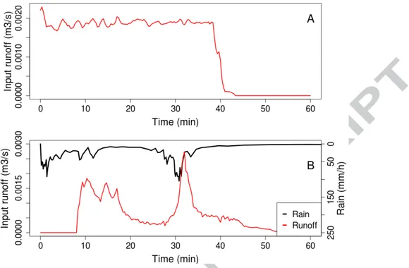
Two monitored events, one artificial and one natural, that show contrasting hydrological behaviours in 106
terms of duration, intensity and generated runoff (Figure 2) were selected for this study. For the artificial 107
event (2006/04/13), 4.5 m3 of water was introduced as surface runoff through gutter 1 for a period of 40
108
minutes. For this event the output hydrograph from gutter 2 was monitored but no surface water reached this 109
point. However, GMS data are available to qualitatively describe surface runoff evolution during the event. To 110
evaluate the subsurface flow, infiltration volume in the lysimeters, continuously monitored for 1 h (i.e., until 111
20 min after the runoff application period), was used. 112
The natural event (2004/09/12) lasted less than one hour and generated a very short runoff output hydro-113
Figure 2: Runoff and rain intensity for the two selected events on the Morcille buffer strip. A: Artificial runoff event (2006/04/13) and B: natural event (2004/09/12).
graph highly connected to the rainfall dynamics (Figure 2 B). The water input for this event included both 114
the precipitation that fell directly on the instrumented field and the runoff input resulting from surface runoff 115
generated on the vineyard plot and collected in gutter 1. In total, 5 m3 of water was introduced, and 0.1 m3
116
of runoff was collected at gutter 2. 117
2.3. Simulation plan 118
The first step of the study aims at understanding the effect of hydraulic conductivity heterogeneity on 119
surface and subsurface fluxes in a buffer strip. We used a homogeneous Ks scenario, a layered (by soil
120
horizon) homogeneous scenario and 5 statistically generated heterogeneous scenarios described in the next 121
section. 60 realizations were performed on each statistically heterogeneous distribution to ensure the stability 122
of the ensemble mean and variance of the response. All simulations were performed for the artificial event of 123
2006/04/13. The results were evaluated for three output variables: surface water volume at three times; 50 124
cm depth infiltration at the lysimeter locations; and spatial distributions of surface ponding. 125
On the basis of the first step analysis, one of the 7 Ks scenarios was selected for the second part of the
126
study, whose aim is to assess also the influence of microtopography. Two microtopography scenarios were 127
generated (see below) and run for 5 realizations from the selected Ks scenario. All simulations, including a
128
third scenario representing the configuration with no microtopography, were performed for the natural event 129
of 2004/09/12. The same output variables as in step 1 were considered, as well as the surface runoff at gutter 130
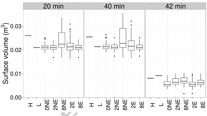
2 (see figure 1). 131
2.3.1. Scenarios for studying the effect of subsurface heterogeneity 132
For the homogeneous (H) and layered homogeneous (L) scenarios we used, respectively, the harmonic 133
average of all measured Ksvalues (4.64e-5 m.s−1) and of the measured Ksvalues by soil horizon (see Table 1).
134
The statistically heterogeneous scenarios were generated using the turning bands toolkit of [61] based on the 135
customary lognormal distribution [41, 43, 44], with mean and standard deviation values for each soil horizon 136
corresponding to the measured data reported in Table 1. Five scenarios were defined for the statistically 137
heterogeneous case: 0, 2 and 8 m horizontal correlation length with no enforcement (0NE, 2NE and 8NE) and 138
2 and 8 m correlation length with enforcement (2E and 8E). For the 2E and 8E scenarios, the Ksdistributions
139
were enforced with the measured values (8 points in horizon 1 and 8 points in horizon 2). The sampling is 140
performed with the turning bands method and enforced by kriging. Exact measurement locations are forced to 141
be respected exactly and their neighbour elements are influenced by their value, depending on their distance 142
to the measurements. Table 2 summarizes the 7 Ks scenarios and Figure 3 shows a realization of the Ks
143
distribution for scenario 8E. 144
Table 2: Summary of the 7 hydraulic conductivity scenarios used in the first step of the study.
Scenario Distribution Horizontal correlation length Enforcement
H homogeneous - -L layered - -homogeneous 0NE 0 m no enforcement 2NE statistically 2 m 8NE generated 8 m 2E heterogeneity 2 m enforcement 8E 8 m
2.3.2. Scenarios for studying the effect of both surface and subsurface heterogeneities 145
Land surface microtopography is highly dependent on soil composition, land use and agricultural prac-146
tices. In absence of accurate radar or lidar field data, microtopography is generally described using fractal 147
distributions for study scales below 1 m2 [62, 63, 64] or Gaussian distributions for larger study scales up to 1
148
ha [65, 46, 51, 47, 48, 49]. In this study we used , based on field observations, a Gaussian distribution with 149
a standard deviation on elevation fluctuations of 3 cm or 6 cm and a mean of zero. A third scenario with 150
no microtopography (corresponding to the hillslope landscape from the first step) was also included in the 151
Figure 3: Example realization of a saturated conductivity field with enforcement points in soil horizons 1 and 2 shown in black. The average Ks for horizons 1, 2 and 3 is, respectively, 1.88e-4 m/s, 4.00e-5 m/s and 1.76e-5 m/s.
analysis. For each of these 3 scenarios, 5 realizations of the selected Ks scenario from step 1 were sampled
152
(labeled Ks1, ..., Ks5). Moreover, for each of the two microtopography distribution scenarios, 5 realizations
153
were sampled (labeled M T 1, ..., M T 5). 154
For all this simulations, the roughness coefficient is kept at the same value because it refers to disturbances 155
or irregularities in the soil surface at a scale which is generally too small to be captured by a conventional 156
topographic map or survey [66]. Manning’s coefficient is an important parameter for sediment transfers as 157
well as for solute transport, but only in a context of gentle slope (less than 5%) [67], which is not the case 158
here. Figure 4 shows an example for the 3 cm scenario. The total number of simulations for the surface and 159
subsurface heterogeneity analysis is thus 55 (5 Ks realizations for the no microtopographic relief case plus 5
160
Ksx 5 M T realizations for each of the 3 cm and 6 cm microtopography cases). No horizontal correlation was
161
used for the microtopography scenarios since observations of the experimental area show that the relief due to 162
grass vegetation is not autocorrelated beyond a length scale of 50 cm, which is the surface mesh size. 163
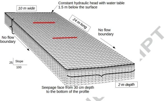
2.4. Model setup 164
In the present study, boundary conditions were assigned according to available field information and were 165
maintained fixed for all simulations. At the upslope lateral boundary, the water table level was maintained at 166
Figure 4: Five realizations of the microtopography field for the scenario with a standard deviation of 3 cm on the elevation fluctuations.
a certain distance below the surface with a Dirichlet condition (fixed hydraulic head), while at the downslope 167
lateral boundary a seepage face was set from 30 cm below the surface to the base of the domain (Figure 5). 168
The initial condition is a hydrostatic equilibrium with a water table matching the upslope boundary condition. 169
The water input was simulated as rainfall on gutter 1 for both the artificial and natural events plus, for the 170
natural event, direct rainfall on the experimental plot as well. The other two lateral boundaries were assigned 171
no flow conditions. Since the simulated domain is larger than the experimental area (see Figure 1), these 172
zero-flux conditions did not unduly influence the simulation results. The land surface was discretized into 20 173
x 48 uniform cells of 50 cm x 50 cm resolution. For the subsurface model each cell was subdivided into two 174
triangles, and the triangular grid was projected vertically over the 2 m soil depth into 15 parallel layers, to 175
produce a 3D mesh of 28800 tetrahedral elements and 16464 nodes. The 15 layers are of variable thickness from 176
1 cm to 15 cm, with the thinnest layers near the surface in order to accurately resolve rainfall-runoff-infiltration 177
partitioning. 178
The water table position was set to 1.5 m below the surface based on available piezometric field data. Given 179
the importance of soil moisture, some preliminary tests were conducted bu simulating the artificial event with 180
three different water table depths as initial condition and considering evapotranspiration (ET) or not. The 181
average ET flux for April for the years 1996 to 2007 is 2.98e−8 m.s−1 (M´et´eo-France). Figures 6A and 6B 182
show that evapotranspiration has no effect on surface water volume evolution through time but its influences 183
on the average moisture in the first 50 cm of soil is apparent as early as the first simulation hours. Concerning 184
the various water table depths, there is a clear difference in average moisture between the 0.5 m, 1 m, 1.5 m 185
water table depth simulations, however all dynamics are similar. This parameter does not have a big impact 186
Figure 5: 3D mesh of the simulated area with applied boundary conditions for the CATHY model (mesh: 50 cm * 50 cm and 15 soil layers). Gutters 1 and 2 are represented in red.
on surface water volume (Figure 6B) and will be kept fixed for the rest of the study. 187
Figure 6: Model setup preliminary tests with various water table depth (WT depth) and evapotranspiration (ET) during the artificial event of 2006/04/13. (A) : average moisture evolution in the first 50 cm of soil through time. (B) : surface water volume evolution through time.
3. Results and discussion 188
3.1. Effect of subsurface heterogeneity 189
The first step of our analysis focuses on subsurface heterogeneity and is performed on the monitored artificial 190
event (Figure 2 A) for the seven subsurface Ksscenarios (Table 2) and the smooth hillslope (no land surface
191
microtopography) configuration. 192
Figure 7: Boxplot of surface water volume at time 20 min, 40 min (end of water input, see Figure 2 A) and 42 min for the seven Ks
scenarios during the artificial event of 2006/04/13. The boxplot results for the 5 statistically heterogeneous scenarios are derived from the 60 realizations that were run for each of these cases.
Figure 7 reports the boxplots of volume of water on the surface, defined as the integral of positive pressure 193
head in regards to the surface, at three times: 20 min (middle of the runoff event), 40 min (end of the runoff 194
event) and 42 min (after the end of the event and before all surface water has infiltrated). Globally, the timing 195
trend is quite homogeneous: the volume of surface water is constant on average during the runoff event and 196
decreases rapidly by the end of the runoff injection at gutter 1. Comparing the homogeneous (H) and layered 197
heterogeneity (L) scenarios, the surface water volume seems to directly depend on the conductivity of the 198
first soil horizon: during the runoff event there is 0.005 m3 more water on the surface for the homogeneous
199
scenario (with Ks = 4.64e-5 m.s−1) than for the layered scenario that has a higher Ks (1.88e-4 m.s−1) in
200
the first horizon. After the injection period this difference decreases and the surface volumes for the H and 201
L simulations are almost equal. For the statistically heterogeneous scenarios, the global mean of the surface 202
water volume follows the L scenario, which indicates again a strong link with average Ksvalue of the first soil
horizon. However, the average of surface water volume stays stable for all heterogeneous scenarios : Ksspatial
204
variability has little influence on this variable. Scenario 8NE (8 m correlation length, no enforcement) stands 205
out as the configuration that produced the most variable and high response in terms of surface water volume 206
over its 60 realizations. 207
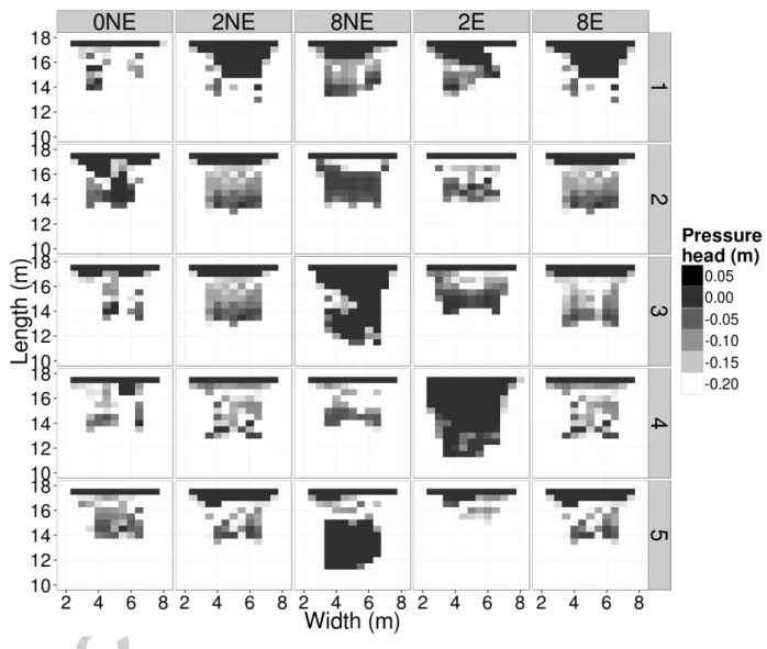
Figure 8: Surface pressure head at t = 40 min for five randomly chosen conductivity realizations from each heterogeneous Ks
scenario during the artificial event of 2006/04/13. Only the experimental plot is represented (see Figure 1), and the axes are given with respect to the model domain.
In addition to its volume, the spatial repartitioning of surface water can also be qualitatively analysed 208
via information obtained form the granular matrix sensors. The GMS data (not shown) indicate a spatial 209
heterogeneity of the surface runoff and a relatively low temporal variability. The simulated spatial surface 210
water repartitioning is shown in Figure 8 in terms of surface pressure head for five realizations of each of the 211
statistically heterogeneous scenarios at t = 40 min. Because the hillslope is smooth, the H and L scenarios, with 212
horizontally homogeneous soils, produced, as expected, a uniform ponding and therefore are not shown. The 213
resulting nonuniform pressure head distributions for all heterogeneous scenarios correspond to the evidence 214
from the GMS observations. As with the surface water volume, the most highly variable ponding patterns 215
(surface pressure heads greater than zero) occur for scenario 8NE. Because the subsurface heterogeneity is 216
randomly generated, none of the simulated ponding patterns show clear runoff pathways. Ks variability,
217
whether between scenarios or realizations, exerts a major influence on surface pressure, and thus on runoff. 218
For some simulations (e.g., scenario 2NE realizations 1 and 5 and scenario 2E realizations 3 and 5, Figure 8) 219
the surface water does not flow more than 3 or 4 m downslope from the injection point at gutter 1. This has 220
consequences on the infiltration process, discussed next. 221
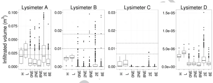
Figure 9: Boxplot of infiltrated volume at the four lysimeter positions and t= 60 min for the seven scenarios of Ks distribution
during the artificial event of 2006/04/13. The simulated values are calculated at 50 cm depth along each of the 9-node transects that align with the lysimeter positions (see Figure 1). The dotted horizontal lines show the range of the measured data.
Figure 9 shows the volume infiltrated in the four lysimeters (see Figure 1) 60 min after the end of the 222
simulation. On the field, each lysimeter is composed of two compartments, which provide two volume values, 223
represented of Figure 9 by the two dotted lines. Note that the volumes measured and simulated at lysimeter 224
D are quite negligible compared to the volumes at lysimeters A, B and C, and that more generally the 225
average infiltrated volume decreases greatly in progressing downslope from lysimeter position A to D. For each 226
lysimeter, the range of infiltrated volumes across the 7 scenarios varies over a much narrower range than from 227
one lysimeter to the next. In contrast to the results for surface water volume, the most variable scenario here 228
is not 8NE but 2E. This implies that the first 50 cm of soil can drastically alter trends observed at the surface. 229
The simulation generally conforms to the field data in lysimeter A and underestimates infiltration in lysimeters 230
B, C and D. 231
In order to examine the interactions between subsurface and surface heterogeneity in the second part of 232
this study, we will focuse on a heterogeneous scenario. On the basis of the lysimeter results, scenario 2E was 233
selected among all heterogeneous scenarios and was applied for the natural rain event of 2004/09/12. 234
3.2. Effect of surface and subsurface heterogeneity 235
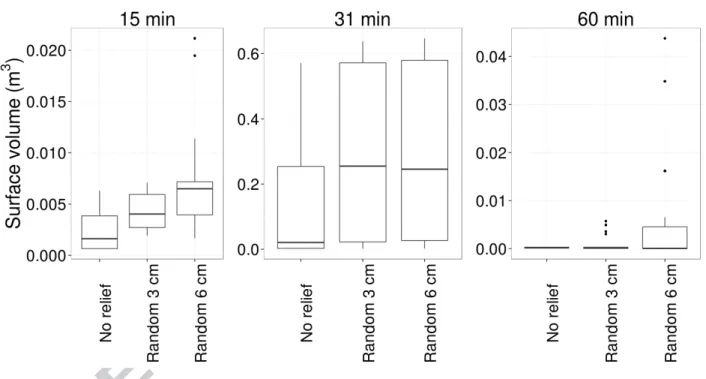
Similarly to the first step of the study, we first compare simulated surface water volume at various times 236
(Figure 10): 15 min (first quarter of the natural event), 31 min (during the hydrograph peak) and 60 min (at 237
the end of the event). The global trend follows a logical sequence for all three microtopography scenarios. At 238
t = 15 min, the surface water volume is less than 0.01 m3, a relatively insignificant amount correponding to
239
less than 0.05 mm over the entire domain. At t = 31 min, during runoff generation, the surface water volume 240
reaches a maximum of 0.6 m3 (average of 2.5 mm of water over the entire simulated surface). By the end of 241
the event, the surface water volume decreases rapidly, which was already observed in the first step. Besides 242
this general trend, it can be seen that the level of ponding increases as the degree of elevation fluctuations 243
increases. 244
Figure 10: Boxplot of surface water volume at three times: 15 min, 31 min (output hydrograph peak) and 60 min for the three scenarios of microtopography heterogeneity during the natural event of 2004/09/12.
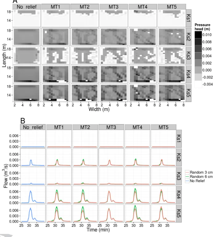
In Figure 11 A, runoff pathways are represented at t = 31 min, the peak of the output hydrograph at 245
gutter 2. In contrast to the first part of the study with a smooth hillslope (Figure 8), preferential runoff 246
pathways are observable when there is microtopographic relief (MT1 to MT5). There is a higher sensitivity 247
to subsurface heterogeneity than to surface heterogeneity, as the variability is greater column-wise (different 248
Ks realizations) than row-wise (MT scenarios). Indeed, the pressure head standard deviation for each node
249
column-wise is three times higher (around 0.01 m) than row-wise (around 0.003 m). The same is also true for 250
the hydrograph response in Figure 11B, and indeed in this case there is also not a great difference between 251
the smooth hillslope, 3 cm microtopography, and 6 cm microtopography cases. This may be due to runoff 252
Figure 11: (A): Surface pressure head (m) at t=31min for the smooth hillslope and for five realizations of the 6 cm microtopography average elevation scenario during the natural event of 2004/09/12. (B): hydrograph output at gutter 2 for all microtopography scenarios during the same event.
response in the surface model being more sensitive to the routing (hydraulic geometry) parameters than to the 253
microtopography characteristics. Surface runoff pathways present different shapes depending on wether the 254
area is flat or not (see figure 11A). Areas with microtopography (as opposed to flat areas) influence the runoff 255
pathway shape by concentrating flows, whereas the surface output hydrograph stays the same (see figure 11A, 256
first column versus all others) : on non-flat areas, a same volume of water infiltrates on a smaller area. 257
Figure 12: Boxplot of infiltrated volume at the four lysimeter positions and t= 90 min for the three microtopography scenarios during the artificial event of 2004/08/12. The simulated values are calculated at 50 cm depth along each of the 9-node transects that align with the lysimeter positions (see Figure 1). The dotted horizontal lines show the range of the measured data.
Figure 12 shows the infiltration volumes in lysimeters A, B, C and D after 90 min (30 min after the end of 258
the event). As with the runoff hydrograph response in Figure 11B, the lysimeter results for the 3 cm and 6 cm 259
microtopography scenarios are comparable in volume and degree of variability. The infiltrated volume for the 260
simulation with a smooth soil surface is higher than with the rough surfaces for all 4 lysimeters, consistent with 261
the lower surface volumes reported in Figure 10 for the smooth hillslope case. Finally, as with the analysis of 262
subsurface heterogeneity in the previous step reported in Figure 9, we again see a general overestimation of 263
the simulated infiltrated volume for lysimeter A compared to the measured data and an underestimation for 264
lysimeters B, C and D. 265
4. Conclusions 266
In this paper, the effect of surface and subsurface heterogeneity representation on water flow in a vegetative 267
buffer strip was assessed. The seven scenarios of saturated hydraulic conductivity simulated with the CATHY 268
model confirmed that conductivity heterogeneity has a significant impact on the buffer strip’s capacity to 269
infiltrate incoming surface runoff. Moreover, enforced scenarios were more consistent with the observations of 270
surface and subsurface responses than the non enforced ones. This result strongly supports the necessity to 271
carefully parameterize hydraulic conductivity by adding information from measurements. In a second step, 272
we examined both surface and subsurface heterogeneity via scenarios combining topographic relief and Ks
273
distributions. The results indicate that the hydrological responses of the buffer strip are much less sensitive 274
to microtopography variability than to Ks variability. This conclusion was observed for variations in both
275
elevation mean and spatial distribution. Microtopography can thus be represented by synthetic distributions, 276
so long as it is not entirely neglected, as is often done due to lack of data. 277
This study focused on Ks and microtopography in representating subsurface and surface heterogeneity,
278
given their importance as suggested by the literature. Other soil characteristics may also be influential, 279
such as initial soil moisture, porosity, roughness, and retention curve parameters. This study approaches the 280
sensitivity analysis idea with few parameters. A rigourous sensitivity analysis of surface runoff and infiltration 281
responses to a wider set of parameters will be conducted in a subsequent study, and will include also an 282
investigation of potential correlations between surface and subsurface heterogeneity. Preferential transfer often 283
accelerates pesticide transfer, depending on the soil structure. Moreover, solute and sediment transfers are 284
in strong interaction with water fluxes on buffer strips. By deliberately focusing on hydrological processes 285
alone in this present study, we have been able to elucidate the combined effects of soil surface and subsurface 286
heterogeneity, at the scale and in the context of a buffer strip. This first study using a physically-based coupled 287
model to examine both surface and subsurface heterogeneity factors has provided some key insights into what 288
variables should be taken into account or neglected in order to properly represent integrated hydrologic fluxes 289
in a vegetative filter. 290
Acknowledgment 291
The authors acknowledge the geostatistical help and advices of E. Leblois. The research for this paper 292
was in part supported by the CMIRA Explora’Doc grant from the Region Auvergne-Rhˆone-Alpes and the 293
LEFE/MANU project ADIMAP. 294
References
[1] N. Poletika, P. Coody, G. Fox, G. Sabbagh, S. Dolder, J. White, Chlorpyrifos and atrazine removal from runoff by vegetated filter strips: Experiments and predictive modeling, Journal of Environmental Quality 38 (3) (2009) 1042–1052. doi:10.2134/jeq2008.0404.
[2] B. Real, J. Mezeray, G. l. Henaff, M. Roettele, et al., Topps-prowadis project: development of diagnosis methods and proposal of practical solutions in order to reduce transfers of plant protection product from run-off and erosion., in: 22e Conf´erence du COLUMA. Journ´ees Internationales sur la Lutte contre les
Mauvaises Herbes, Dijon, France, 10-12 d´ecembre 2013., Association Fran¸caise de Protection des Plantes (AFPP), 2013, pp. 672–681.
[3] M. G. Dosskey, Toward quantifying water pollution abatement in response to installing buffers on crop land, Environmental Management 28 (5) (2001) 577–598. doi:10.1007/s002670010245.
[4] A. L. Fox, D. E. Eisenhauer, M. Dosskey, Modeling water and sediment trapping by vegetated filters using VFSMOD: Comparing methods for estimating infiltration parameters, USDA Forest Service/UNL Faculty Publications. (2005) nadoi:10.13031/2013.18934.
[5] A. Carter, Herbicide movement in soils: principles, pathways and processes, Weed Research 40 (1) (2000) 113–122. doi:10.1046/j.1365-3180.2000.00157.x.
[6] J.-G. Lacas, Processus de dissipation des produits phytosanitaires dans les zones tampons enherb´ees: ´etude exp´erimentale et mod´elisation en vue de limiter la contamination des eaux de surface, Ph.D. thesis, Montpellier 2 (2005).
[7] J.-G. Lacas, N. Carluer, M. Voltz, Efficiency of a grass buffer strip for limiting diuron losses from an uphill vineyard towards surface and subsurface waters, Pedosphere 22 (4) (2012) 580–592. doi:10.1016/ S1002-0160(12)60043-5.
[8] J.-G. Lacas, M. Voltz, V. Gouy, N. Carluer, J.-J. Gril, Using grassed strips to limit pesticide transfer to surface water: a review, Agronomy for Sustainable Development 25 (2) (2005) 253–266.
[9] D. Lee, T. D. Dillaha, J. H. Sherrard, Modeling phosphorus transport in grass buffer strips, Journal of Environmental Engineering 115 (2) (1989) 409–427. doi:10.1061/(ASCE)0733-9372(1989)115:2(409). [10] R. Munoz-Carpena, J. E. Parsons, J. Gilliam, Modeling hydrology and sediment transport in vegetative
filter strips, Journal of Hydrology 214 (14) (1999) 111–129. doi:10.1016/S0022-1694(98)00272-8. [11] J. Simunek, M. Sejna, M. van Genuchten, The HYDRUS-2D software package for simulating
two-dimensional movement of water, heat, and multiple solutes in variably-saturated media, Version 2.0, US Salinity Laboratory, USDA, ARS, Riverside.
[12] C. Yu, C. Zheng, Hydrus: Software for flow and transport modeling in variably saturated media, Ground Water 48 (6) (2010) 787–791. doi:10.1111/j.1745-6584.2010.00751.x.
[13] J. M. Koehne, T. Woehling, V. Pot, P. Benoit, S. Leguedois, Y. L. Bissonnais, J. Simunek, Coupled simulation of surface runoff and soil water flow using multi-objective parameter estimation, Journal of Hydrology 403 (12) (2011) 141–156. doi:10.1016/j.jhydrol.2011.04.001.
[14] M. Abu-Zreig, Factors affecting sediment trapping in vegetated filter strips: simulation study using VFS-MOD, Hydrological Processes 15 (8) (2001) 1477–1488. doi:10.1002/hyp.220.
[15] A. Sovik, P. Aagaard, Spatial variability of a solid porous framework with regard to chemical and physical properties, Geoderma 113 (1) (2003) 47–76. doi:10.1016/S0016-7061(02)00315-4.
[16] M. Herbst, B. Diekkrueger, J. Vanderborght, Numerical experiments on the sensitivity of runoff generation to the spatial variation of soil hydraulic properties, Journal of Hydrology 326 (1) (2006) 43–58. doi: 10.1016/j.jhydrol.2005.10.036.
[17] M. M. Gribb, Parameter estimation for determining hydraulic properties of a fine sand from transient flow measurements, Water Resources Research 32 (7) (1996) 1965–1974. doi:10.1029/96WR00894.
[18] T.-C. J. Yeh, J. Zhang, A geostatistical inverse method for variably saturated flow in the vadose zone, Water Resources Research 32 (9) (1996) 2757–2766. doi:10.1029/96WR01497.
[19] S. Boateng, Evaluation of probabilistic flow in two unsaturated soils, Hydrogeology Journal 9 (6) (2001) 543–554. doi:10.1007/s10040-001-0164-6.
[20] J. Mertens, H. Madsen, M. Kristensen, D. Jacques, J. Feyen, Sensitivity of soil parameters in unsaturated zone modelling and the relation between effective, laboratory and in situ estimates, Hydrological Processes 19 (8) (2005) 1611–1633. doi:10.1002/hyp.5591.
[21] J. Simunek, M. van Genuchten, M. M. Gribb, J. W. Hopmans, Parameter estimation of unsaturated soil hydraulic properties from transient flow processes, Soil and Tillage Research 47 (1) (1998) 27–36. doi:10.1016/S0167-1987(98)00069-510.1016/S0167-1987(98)00069-5.
[22] F. Abbasi, J. Feyen, M. T. van Genuchten, Two-dimensional simulation of water flow and solute transport below furrows: model calibration and validation, Journal of Hydrology 290 (1) (2004) 63–79. doi:10. 1016/j.jhydrol.2003.11.028.
[23] C. Dages, M. Voltz, P. Ackerer, Parameterization and evaluation of a three-dimensional modelling ap-proach to water table recharge from seepage losses in a ditch, Journal of Hydrology 348 (3) (2008) 350–362. doi:10.1016/j.jhydrol.2007.10.004.
[24] X. Liang, Z. Xie, A new surface runoff parameterization with subgrid-scale soil heterogeneity for land surface models, Advances in Water Resources 24 (9–10) (2001) 1173–1193. doi:10.1016/S0309-1708(01) 00032-X.
[25] V. Polyakov, A. Fares, M. H. Ryder, Precision riparian buffers for the control of nonpoint source pollutant loading into surface water: A review, Environmental Reviews 13 (3) (2005) 129–144. doi:10.1139/ a05-010.
[26] K. Moser, C. Ahn, G. Noe, Characterization of microtopography and its influence on vegetation patterns in created wetlands, Wetlands 27 (4) (2007) 1081–1097. doi:10.1672/0277-5212(2007)27[1081:COMAII] 2.0.CO;2.
[27] B. P. Mohanty, M. D. Ankeny, R. Horton, R. S. Kanwar, Spatial analysis of hydraulic conductivity measured using disc infiltrometers, Water Resources Research 30 (9) (1994) 2489–2498. doi:10.1029/ 94WR01052.
[28] K. J. Beven, E. F. Wood, M. Sivapalan, On hydrological heterogeneity : Catchment morphology and catch-ment response, Journal of Hydrology 100 (13) (1988) 353–375. doi:10.1016/0022-1694(88)90192-8. [29] M. B. Ceddia, S. R. Vieira, A. L. O. Villela, L. d. S. Mota, L. H. C. Anjos, D. F. Carvalho, Topography
and spatial variability of soil physical properties, Scientia Agricola 66 (2009) 338–352. doi:10.1590/ S0103-90162009000300009.
[30] D. Mulla, Variability in soil properties from soil classification, in: A. W. Warrick (Ed.), Soil Physics Companion, Taylor & Francis Group, Boca Raton, 2010, Ch. 9, pp. 343–344.
[31] D. A. Woolhiser, R. E. Smith, J.-V. Giraldez, Effects of spatial variability of saturated hydraulic conductivity on Hortonian overland flow, Water Resources Research 32 (3) (1996) 671–678. doi: 10.1029/95WR03108.
[32] A. Sole-Benet, A. Calvo, A. Cerda, R. Lazaro, R. Pini, J. Barbero, Influences of micro-relief patterns and plant cover on runoff related processes in badlands from Tabernas (SE Spain), Catena 31 (1-2) (1997) 23–38. doi:10.1016/S0341-8162(97)00032-5.
[33] P. Van Der Keur, B. V. Iversen, Uncertainty in soil physical data at river basin scale ? a review, Hydrology and Earth System Sciences Discussions 10 (6) (2006) 889–902.
URL https://hal.archives-ouvertes.fr/hal-00305034
[34] J. Sobieraj, H. Elsenbeer, G. Cameron, Scale dependency in spatial patterns of saturated hydraulic con-ductivity, Catena 55 (1) (2004) 49–77. doi:10.1016/S0341-8162(03)00090-0.
[35] P. Cook, G. Walker, I. Jolly, Spatial variability of groundwater recharge in a semiarid region, Journal of Hydrology 111 (1) (1989) 195–212. doi:10.1016/0022-1694(89)90260-6.
[36] D. Russo, E. Bresler, Soil hydraulic properties as stochastic processes: I. an analysis of field spatial variability, Soil Science Society of America Journal 45 (4) (1981) 682–687. doi:10.2136/sssaj1981. 03615995004500040002x.
[37] L. Chen, S. Sela, T. Svoray, S. Assouline, The role of soil-surface sealing, microtopography, and vegetation patches in rainfall-runoff processes in semiarid areas, Water Resources Research 49 (9) (2013) 5585–5599. doi:10.1002/wrcr.20360.
[38] S. Frei, G. Lischeid, J. Fleckenstein, Effects of microtopography on surface subsurface exchange and runoff generation in a virtual riparian wetland. a modeling study, Advances in Water Resources 33 (11) (2010) 1388–1401. doi:10.1016/j.advwatres.2010.07.006.
[39] M. Seyfried, Spatial variability constraints to modeling soil water at different scales, Geoderma 85 (2–3) (1998) 231–254. doi:10.1016/S0016-7061(98)00022-6.
[40] A. Samouelian, I. Cousin, C. Dages, A. Frison, G. Richard, Determining the effective hydraulic properties of a highly heterogeneous soil horizon, Vadose Zone Journal 10 (1) (2011) 450–458. doi:doi:10.2136/ vzj2010.0008.
[41] G. Dagan, E. Bresler, Unsaturated flow in spatially variable fields: 1. derivation of models of infiltration and redistribution, Water Resources Research 19 (2) (1983) 413–420. doi:10.1029/WR019i002p00413. [42] H. M. Abdou, M. Flury, Simulation of water flow and solute transport in free-drainage lysimeters and
field soils with heterogeneous structures, European Journal of Soil Science 55 (2) (2004) 229–241. doi: 10.1046/j.1365-2389.2004.00592.x.
[43] J. R. Craig, G. Liu, E. D. Soulis, Runoff infiltration partitioning using an upscaled Green-Ampt solution, Hydrological Processes 24 (16) (2010) 2328–2334. doi:10.1002/hyp.7601.
[44] R. S. Govindaraju, C. Corradini, R. Morbidelli, Local- and field-scale infiltration into vertically non-uniform soils with spatially-variable surface hydraulic conductivities, Hydrological Processes 26 (21) (2012) 3293–3301. doi:10.1002/hyp.8454.
[45] D. Pasetto, G.-Y. Niu, L. Pangle, C. Paniconi, M. Putti, P. A. Troch, Impact of sensor failure on the observability of flow dynamics at the Biosphere 2 LEO hillslopes, Advances in Water Resources 86 (2015) 327–339. doi:10.1016/j.advwatres.2015.04.014.
[46] B. Zinn, C. F. Harvey, When good statistical models of aquifer heterogeneity go bad: A comparison of flow, dispersion, and mass transfer in connected and multivariate Gaussian hydraulic conductivity fields, Water Resources Research 39 (3) (2003) na. doi:10.1029/2001WR001146.
[47] M. Antoine, M. Javaux, C. L. Bielders, Integrating subgrid connectivity properties of the microtopography in distributed runoff models, at the interrill scale, Journal of Hydrology 403 (2011) 213–223. doi:10. 1016/j.jhydrol.2011.03.027.
[48] W. M. Appels, P. W. Bogaart, S. E. van der Zee, Influence of spatial variations of microtopography and infiltration on surface runoff and field scale hydrological connectivity, Advances in Water Resources 34 (2) (2011) 303–313. doi:10.1016/j.advwatres.2010.12.003.
[49] J. Yang, X. Chu, A new modeling approach for simulating microtopography-dominated, discontinuous overland flow on infiltrating surfaces, Advances in Water Resources 78 (2015) 80–93. doi:10.1016/j. advwatres.2015.02.004.
[50] P. M. Atkinson, N. J. Tate, Spatial scale problems and geostatistical solutions: A review, The Professional Geographer 52 (4) (2000) 607–623. doi:10.1111/0033-0124.00250.
[51] S. E. Thompson, G. G. Katul, A. Porporato, Role of microtopography in rainfall-runoff partitioning: An analysis using idealized geometry, Water Resources Research 46 (7) (2010) na. doi:10.1029/ 2009WR008835.
[52] S. Anderton, J. Latron, F. Gallart, Sensitivity analysis and multi-response, multi-criteria evaluation of a physically based distributed model, Hydrological Processes 16 (2) (2002) 333–353. doi:10.1002/hyp.336. [53] C. Paniconi, M. Putti, Physically based modeling in catchment hydrology at 50: Survey and outlook,
Water Resources Research 51 (9) (2015) 7090–7129. doi:10.1002/2015WR017780.
[54] M. Camporese, C. Paniconi, M. Putti, S. Orlandini, Surface-subsurface flow modeling with path-based runoff routing, boundary condition-based coupling, and assimilation of multisource observation data, Water Resources Research 46 (2) (2010) W02512. doi:10.1029/2008WR007536.
[55] C. Paniconi, M. Putti, A comparison of Picard and Newton iteration in the numerical solution of mul-tidimensional variably saturated flow problems, Water Resources Research 30 (12) (1994) 3357–3374. doi:10.1029/94WR02046.
[56] S. Orlandini, G. Moretti, M. Franchini, B. Aldighieri, B. Testa, Path-based methods for the determination of nondispersive drainage directions in grid-based digital elevation models, Water Resources Research 39 (6) (2003) na.
[57] M. C. Peel, B. L. Finlayson, T. A. McMahon, Updated world map of the K¨oppen-Geiger climate classifi-cation, Hydrol. Earth Syst. Sci. 11 (5) (2007) 1633–1644. doi:10.5194/hess-11-1633-2007.
[58] R. VandenBogaert, Typologie des sols du bassin versant de la Morcille, caract´eristation de leurs propri´et´es hydrauliques et test de fonctions de pedotranfert., Master’s thesis, Universit´e Pierre et Marie Curie & AgroParisTech (2011).
[59] E. P. Eldredge, C. C. Shock, T. D. Stieber, Calibration of granular matrix sensors for irrigation manage-ment, Agronomy Journal 85 (6) (1993) 1228–1232. doi:10.2134/agronj1993.00021962008500060025x. [60] M. T. van Genuchten, A closed-form equation for predicting the hydraulic conductivity of unsaturated
soils, Soil Science Society of America Journal 44 (5) (1980) 892–898.
[61] E. Leblois, J.-D. Creutin, Space-time simulation of intermittent rainfall with prescribed advection field: Adaptation of the turning band method, Water Resources Research 49 (6) (2013) 3375–3387. doi: 10.1002/wrcr.20190.
[62] G. Pardini, F. Gallart, A combination of laser technology and fractals to analyse soil surface roughness, European Journal of Soil Science 49 (2) (1998) 197–202. doi:10.1046/j.1365-2389.1998.00149.x. [63] F. Darboux, C. Gascuel-Odoux, P. Davy, Effects of surface water storage by soil roughness on overland-flow
generation, Earth Surface Processes and Landforms 27 (3) (2002) 223–233. doi:10.1002/esp.313. [64] F. S. J. Martinez, J. Caniego, A. Guber, Y. Pachepsky, M. Reyes, Multifractal modeling of soil
micro-topography with multiple transects data, Ecological Complexity 6 (3) (2009) 240–245. doi:10.1016/j. ecocom.2009.05.002.
[65] J. K. Mitchell, B. A. Jones, Microrelief surface depression storage: Analysis of models to describe the depth-storage function1, Journal of the American Water Resources Association 12 (6) (1976) 1205–1222. doi:10.1111/j.1752-1688.1976.tb00256.x.
[66] G. Govers, I. Takken, K. Helming, Soil roughness and overland flow, Agronomie 20 (2) (2000) 131–146. doi:10.1051/agro:2000114.
[67] R. Munoz-Carpena, G. A. Fox, G. J. Sabbagh, Parameter importance and uncertainty in predicting runoff pesticide reduction with filter strips, Journal of environmental quality 39 (2) (2010) 630 641.
Effect of surface and subsurface heterogeneity on the hydrological response of
a grassed buffer zone
Highlights :
• Heterogeneous saturated conductivity (Ks) reflects the complexity of buffer strips. • Field data-enforced model parameterization improves consistency with observations. • Hydrological responses are more sensitive to Ks than to microtopography variability.
![Table 1: Soil hydrodynamic properties for the Morcille buffer strip (after [6]). n, θ r and ψ sat are the parameters for the van](https://thumb-eu.123doks.com/thumbv2/123doknet/2948930.80056/6.918.106.823.580.820/table-soil-hydrodynamic-properties-morcille-buffer-strip-parameters.webp)