Abstract-- This paper proposes a methodology for the design of
automatic load shedding against voltage instability. In a first step, we describe a method allowing to find the minimal shedding required in a given unstable scenario. In a second step, we describe the structure of various controllers and identify the parameters to be optimized. Next, we present an optimization approach to find the controller parameters which optimize an overall performance objective. Results are presented on the Hydro-Québec system, in which load shedding is presently planned.
Index Terms-- Voltage stability, system protection schemes,
load shedding, combinatorial optimization I. INTRODUCTION
N the deregulated*environment and owing to the difficulty of building new transmission and generation facilities, power systems will be operated closer to their stability limits. There are two lines of defence against incidents likely to trigger such instabilities:
i Preventively : estimate security margins with respect to credible contingencies, i.e. incidents with a reasonable probability of occurrence, and take appropriate preventive actions to restore sufficient margins when needed;
i Correctively : implement automatic corrective actions, through System Protection Schemes (SPS), to face the more severe, but less likely incidents [1].
Preventive security criteria usually require that the system remains stable after any credible contingency, without the help of corrective actions. The main reason is that these actions usually affect generators and/or loads, which is acceptable only in the presence of severe disturbances.
The present paper concentrates on long-term voltage instability, driven by Load Tap Changers (LTCs), generator OverExcitation Limiters (OELs), switched shunt compensation, restorative loads, and possibly secondary voltage control. This type of instability has become a major threat in many systems [2], [3].
Since long-term voltage instability is triggered mainly by the loss of generation or transmission facilities, ``N-1'' contingencies corresponding to the loss of a single equipment are usually considered in preventive security analysis. On the other hand, N-2 and more severe disturbances should be
* T. Van Cutsem is a research director of F.N.R.S. (Belgian Funds for Scientific
Research), C. Moors is a F.R.I.A. researcher
counteracted by an SPS. While it must be used in the last resort and to the least extent, automatic load shedding is very effective in this respect.
A few undervoltage load shedding schemes have been proposed or implemented throughout the world (e.g. [1], [4], [5]). This paper compares three types of closed-loop load shedding controllers in terms of performances and design computational effort. The first two controllers are local by nature: they rely on local measurements taken from the system and shed loads once the observed signal stays below some threshold for some time. The third controller is a step towards a wide-area protection, in the sense that other post-disturbance corrective controls are handled in addition to load shedding.
This paper is organized as follows. Section II describes how the optimal load shedding is determined in a given unstable scenario. Section III describes the common structure of the various controllers, while Section IV explains how their various parameters are optimized. Section V compares the performances of the controllers on a rather complex example taken from the Hydro-Québec system. Conclusions and perspectives are presented in Section VI.
II. DETERMINATION OF OPTIMAL LOAD SHEDDING
Location, amount and delay are the three main characteris-tics of load shedding. Obviously the amount of load shedding should be minimal.
For a given shedding delay and location, the minimal amount of shedding Pcan be simply determined by binary or
incremental search, resorting to time-domain simulations to check the system behaviour. As far as long-term voltage stability is concerned, the computing times can be dramatically reduced by using the Quasi Steady-State (QSS) simulation technique. This well-documented approach is based on time decomposition and consists of replacing the short-term dynamics by equilibrium equations, while focusing on the long-term dynamics [3].
The next point is to determine which delay and location yield the smallest amount P*P These two problems are discussed
separately hereafter.
A. Optimizing the shedding delay
One motivation for delaying load shedding is to ascertain that the system is indeed voltage unstable, and hence to avoid shedding load unduly.
Design of Load Shedding Schemes against
Voltage Instability using Combinatorial Optimization
I
T. Van Cutsem* C. Moors* D. Lefebvre**
*University of Liège, Institut Montefiore **Hydro-Québec, Division Transénergie Sart Tilman B37, B-4000 Liège, Belgium CP 10000 Montréal (QC), Canada [email protected] [email protected]
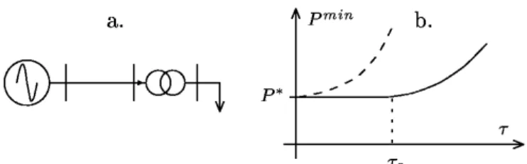
The influence of the delay τ(counted from the disturbance inception) on the minimal amount of power to shed Pmin can be easily established for the simple one machine-one load system of Fig. 1.a [6]. Assuming that the load obeys the well-known exponential model in the short term and restores to constant power in the long term, due to LTC effect, the following can be concluded [6] (Fig. 1.b):
- Pmin remains constant as far as load shedding takes place before some critical time τc. This constant value, denoted P*, is the load decrease just needed to create a long-term equilibrium in the post-contingency configuration;
- if shedding takes place after τc, more load has to be shed; this is a matter of attraction towards the newly created long-term equilibrium.
Note however that a severe disturbance may yield the dashed characteristic of Fig. 1.b, in which Pmin increases right away with the shedding delay τ, i.e. τc = 0.
Fig. 1. Theoretical shedding characteristic of a one machine-one load system
According to the authors’ experience, large real-life systems have Pmin(τ) characteristics quite close to the above described ones, as far as long-term dynamics is governed by OELs, LTCs and secondary voltage control (if any) [6].
On the other hand, the characteristic may change when other post-contingency controls “compete” with load shedding. In this case, it may be advantageous to delay load shedding so that these controls act first and hence less load is shed. An example is provided in Fig. 2, relative to the Hydro-Québec system considered in Section V. In this system, automatic shunt reactor tripping significantly contributes to stabilizing the system in its post-contingency configuration. The figure shows that 280 MW load are saved when the shedding is delayed by 16 seconds, allowing 2970 Mvar to be tripped before load is shed.
Fig. 2. A shedding characteristic on the Hydro-Québec system
In the design of a load shedding protection, we will use the minimum P* as a target value.
B. Optimizing with respect to the shedding location
Small-disturbance analysis coupled with time-domain simulation [6] is used to identify the best shedding location. Along the unstable trajectory provided by this time-domain method, sensitivity analysis is used to identify the critical point, at which the eigenvector corresponding to the (almost) zero eigenvalue is computed. This information allows to obtain a ranking of load buses with respect to the efficiency of load shedding. A given amount of load shedding is distributed over the buses in this order, taking into account the interruptible fraction of each load.
In this approach, a coupling between time-domain simulation and small-disturbance analysis is necessary. This coupling in easier with QSS simulation which is free from short-term transients.
III. STRUCTURE OF THE CONTROLLERS
All protections considered in this paper rely on a measured signal which is typically the average voltage V over several transmission buses in the load area of concern. Other measurements could also enter the logic, such as the reactive reserve of neighbouring generators, etc. Individual loads are shed according to a predefined bus ranking, determined as outlined is section IV.A. It must be emphasized that each protection operates in closed-loop since V is continuously measured and the protection may trigger several, successive load sheddings, if needed.
A. Fixed-Steps Fixed Delays (FSFD) controller.
The first type of controller relies on k rules, each of the type: if V < Vimin during di seconds, shed ∆Pi MW
The number k of rules is decided a priori; in practice it is typically equal to 2 or 3.
A two-rule example from the Hydro-Québec system is given in Fig. 3, in which a star indicates a shunt compensation switching and Rx a load shedding due to rule Rx. As can be seen, the total shedding results from two firings of R2, followed by one firing of R1.
Fig. 3 2-rule protection example from the Hydro-Québec system
Note also that the above rules are ``concurrent''. In the case of Fig. 3, for instance, both rules have their ``if clause'' satisfied just after the disturbance. Due to its much larger timing, R1 is not fired before being reset (at t=12 s) under the effect of R2.
The optimization of such a controller consists in properly determining the 3k-dimensional vector of unknows:
x = [V1min, d1, ∆P1, ..., Vkmin, dk, ∆Pk] (1) Clearly, it is required to adjust the amount of load shedding to the severity of the situation. To meet this objective, the above controller must be provided with either a very fast acting rule (which may interact with the other rules) or additional rules (which significantly increase the use of the next design.
B. Variable-Step Variable Delay (VSVD) controller
The second type of controllers is a kind of generalization of the previous one. It relies on a unique rule whose activation delay d and amount of shed load ∆P depend on the time evolution of V. The idea is to set up a controller adjusting its action automatically to the severity of the situation it is facing: the faster the decrease in V, the shorter d and the larger ∆P.
Thus, the delay d is such that:
dmin d dmax d t t C dt ) V V ( 0 0 ≤ ≤ + = −
∫
min with (2)where t0 is the time at which V becomes smaller than Vmin and C is a constant to be optimized at the design stage.
In the same manner, the load shedding step is given by: ∆P=k∆Vavg with ∆Pmin ≤∆P≤∆Pmax (3) where ∆Vavg is the average voltage drop over the [t0 t0+d] interval: t t min d 1 0 0 dt d ) V V ( avg V
∫
+ − = ∆Two variants of this controller have been considered: • the Variable-Step Fixed Delay (VSFD) controller works with a constant delay d and sheds load according to (3);
• in the Fixed-Step Variable Delay (FSVD) controller, the delay is adjusted using the inverse-time charcteristic (2) while the shedding step ∆P constant.
The optimization requires the determination of one of the following vectors, depending on the variant considered:
xVSVD = [Vmin, C, dmin, dmax, k, ∆ Pmin, ∆ Pmax] (4)
xFSVD = [Vmin, C, dmin, dmax, ∆ P] (5)
xVSFD = [Vmin, C, d, k, ∆ Pmin, ∆ Pmax] (6) C. Coordinated controller
As is well known, several post-disturbance actions are possible to counteract voltage instability. Among them, shunt compensation switching is the first to come to mind. In the example of Fig. 1, the pre-existing shunt reactor tripping scheme has been taken into account when optimizing the settings of the two-rule controller. In other words, the optimization has implicitly taken the most benefit from the imposed compensation.
In the last type of controllers, a more general viewpoint is adopted by coordinating load shedding together with the other post-disturbance corrective controls, thereby approaching a notion of wide-area protection.
The logic is based on several rules. The first one relates to load shedding and is the same as for the VSVD, VSFD or FSVD controller. The other rules are associated to the other corrective controls handled by the protection. In this work, we have considered shunt compensation switching in addition to load shedding. The following rule is used to decide the switching of the compensations:
if V < Vsh during δ (or δ ') seconds, switch one more shunt Preliminary simulations showed that the controller should trip shunt reactors as soon as possible in order to minimize the amount of shed load. This is why we introduce two delays, δ and δ‘, respectively. δ ' relates to the (short) time period between two successive switchings, while δ refers to the (larger) delay preceding the first action. The value of the latter has to be carefully chosen in order the controller not to respond to temporary voltage drops.
In this scheme, we also have to determine the location where compensation has to be switched. To this purpose, transmission bus voltages are checked each time the rule has to be fired and compensation is switched at the bus with the lowest voltage.
The optimization of this controller requires the determination of the Vsh, δ and δ' parameters together with the ones relative to the load shedding rule (4), (5) or (6).
IV. DESIGN OF THE CONTROLLERS
The methodology used to adjust the settings of the various controllers consists of two steps. In the first step, a set of training scenarios is built, and each unstable scenario of this set is analyzed to determine the minimal load shedding which stabilizes the system. In the second step, the protection parameters are determined in order to approach as closely as possible the optimal sheddings computed in the first step, over the whole set of scenarios. A combinatorial optimization method is used to this purpose.
A. Scenario analysis
The first step of our approach consists in setting up a set of s training scenarios, corresponding to various topologies, load levels, generation schemes, contingencies, etc.
In principle all the scenarios to be dealt with by a single protection should involve the same weak area of the system. In other words, the instability modes and hence the optimal shedding locations should be rather close for all the unstable scenarios of the set. Therefore, we assume that a common bus ranking can be set up, e.g. through eigenvector analysis, as mentioned in section II.B. Once this ranking has been identified, the minimal amount of load shedding Pi* (i=1,...,s) is determined for each scenario.
It must be emphasized that the Pi* values depend on the (automatic) shunt compensation switching sequences. When optimizing the FSFD or VSVD controllers, the settings of the compensation control devices are fixed (at their existing
values); therefore, Pi* can be determined by varying the amount and delay of load shedding, using the procedure described in section II.A. On the other hand, when optimizing the coordinated controller, shunt compensation becomes itself a degree of freedom, which makes the determination of Pi* more complex. To keep the problem tractable, we have made the reasonable assumption that the faster the shunt compensation switching, the lower the minimal amount to shed. The Pi* values are therefore computed by assuming that the whole compensation is switched just after the disturbance occurrence. B. Statement of the design problem
Given the s training scenarios, the problem is to determine the vector of unknowns x relative to the controller of concern, such that the following requirements are met:
1. the amount of load shedding must be as close as possible to
the minimum Pi* determined in the first step;
2. all unstable scenarios must be saved (dependability); 3. no load must be shed in a stable scenario (security);
4. optionally, some other constraints can be imposed. For
instance, the distribution voltages should not stay below some threshold for more than some time.
This can be translated into an optimization problem: minimize the discrepancies Pish(x)- Pi*, where Pish(x) is the total load power shed in the i-th scenario (a function of x). Among the possible objective functions, we pay attention to the L1 norm:
∑
= + − s 1 i )] ( i p * i P ) ( sh i P [ s 1 min x x x (7)as well as the L∞ norm:
min max[Pish(x) Pi* pi(x)]
x i − + (8) where the sum and the max extend over the unstable scenarios and pi(x) is a penalty term accounting for the violation of the above requirements. Note that in (7) and (8), the expression within brackets is always positive since Pish > Pi* and pi(x) ≥0.
The penalties are chosen as follows:
• when the system is unstable (requirement 2 violated), transmission voltages eventually become smaller than some threshold Vlow. Denoting by tlow the time at which this occurs, the penalty takes on the form:
1 with C1 ff0 andC2 f0 2 C low t C i p + = (9)
• when an amount Pish is shed in a stable case (requirement 3 violated), the penalty term takes on the form:
pi =C3 Pish(x) with C3 ff1 (10) • let trec be the recovery time, i.e. the time at which voltages are again larger than a specified value. Requirement 4 consists in specifying that trec is smaller than a given value trecmax. If this does not hold, the penalty is taken as:
pi =C4(trec-trecmax) with C3 ff0 (11) Note that with the above penalties, the more dangerous a situation (i.e. the shorter tlow or the larger trec), the higher the
penalty. This is expected to provide the optimization method with information on how to improve the parameters.
C. The branch-and-bound approach
The optimization problem (7-11) is complex. Indeed, both Pish and pi must be determined from time-domain simulations and hence, explicit analytical expressions cannot be established. Moreover, they vary with x in a discontinuous manner, which prevents from using analytical optimization methods. Finally, multiple local minima are expected. This is why we prefer to resort to combinatorial optimization.
To this purpose, each component of x is discretized in a finite number of possible values. The discretization steps are chosen in accordance with the engineering knowledge of the problem (see section V.B).
A brute-force approach would consist in evaluating the objective function for all possible values of x and selecting the best one as solution of the problem, as detailed in Fig. 4, with the bold type line ignored for the time being.
Note that the evaluation of L1 or L∞ for a given protection setting requires the simulation of the s scenarios in order to compute the s discrepancies Pish(x)-Pi*+pi(x), which is very time consuming. Accordingly, this approach cannot be envisaged in real-life problems.
However, this brute force enumeration can be significantly improved in the following way. In the above algorithm, during the enumeration we keep track of the best objective B reached so far. This value B is an upper bound on the sought global minimum. Therefore, in the course of computing the L1 or L∞ objective, as soon as the latter becomes greater than B, we can skip the current value of x and proceed with the next one (see the bold type line in Fig. 4). Indeed, since the objective function can only increase with the number of processed scenarios, the current x can only lead to an objective larger than B.
Fig. 4. Purely enumerative and branch-and-bound approaches
This significant short-cut of the enumerative search is nothing but an application of the branch-and-bound technique [7]. Note that in the case of the FSFD controller, the optimization problem can be formulated as a tree exploration and the branch-and-bound algorithm can be further improved as detailed in [8].
V. RESULTS ON THE HYDRO-QUÉBEC SYSTEM
The Hydro-Québec (HQ) network is characterized by great distances (more than 1000 km) between the large hydro generation areas in the North and the main load center in the South, where the system is voltage stability limited. In order to upgrade the reliability of its transmission system, HQ is deploying a defence plan against extreme contingencies. This plan includes shunt reactor tripping devices, known under the French acronym MAIS, which control a large part of the total 25,500 Mvar shunt compensation. Each MAIS relies on one bus voltage, the coordination between substations being performed through the switching delays.
A. Training Scenarios
Table 1. Configurations considered in the training scenarios
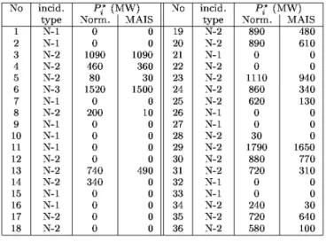
Tables 1 and 2 detail the 8 system configurations and the 36 scenarios finally selected. They involve N-1, N-2 and N-3 contingencies, respectively. In accordance with the standard operating rules, the system is stable following any N-1 incident. The MAIS devices can be used to this purpose.
Table 2. Description of the 36 training scenarios
In each unstable scenario, the best load shedding location has been identified. Therefrom, a common ranking of load buses has been set up. Using this bus ranking, the minimal amount of load shedding Pi* required to stabilize the system has been determined in the 19 unstable scenarios. The values, computed with an accuracy of 10 MW, are given in Table 2. The most severe incident requires to shed load at 8 buses.
In this determination, we supposed that reactors are tripped: • either all together just after the disturbance, as discussed in section IV.A (results given in the ``MAIS'' column);
• or by the MAIS controllers, as implemented presently in the HQ system (results given in the ``Norm.'' column).
The scenarios have been chosen according to the following guidelines:
• the training set includes 17 stable scenarios in order to train the protection not to act in stable cases;
• on the other hand, the nonzero values of Pi* range rather uniformly in the [0 1790] MW interval, between the marginally and the severely unstable cases.
The measured signal V is the average voltage over five 735-kV buses in the Montréal area. Requirements 1, 2 and 3 of Section IV.B have been taken into account. However, in accordance with Hydro-Québec planning rules, the third requirement has been amended by allowing some (hopefully small) load shedding to take place after a stable but severe incident. The N-2 scenarios No 12, 17, 18 and 22 are concerned. The latter are handled as unstable scenarios with Pi* = 0 in (7) and (8).
B. Preliminary choices of controller parameters
In order to obtain a good synchronization with MAIS devices whose settings are typically in the range [0.965 0.97 pu], the V1min parameter of (1) and the Vmin parameters of (4-6) were adjusted to 0.95 pu. Moreover, this value guarantees that the controllers will not act in the stable situations of Table 2, except for scenario 10 whose voltage falls below 0.93 pu at the beginning of the simulation. In the case of 2- or 3-rule controllers, the thresholds relative to rules 2 and 3 were adjusted to 0.93 and 0.91 pu respectively, in order to act before the amount of shed load becomes prohibitive and also to minimize the customers' trouble.
For each kind of controller, the lower bound on each delay is fixed to 3 s in order to distinguish a voltage instability from a temporary undervoltage. The lower bound on load shedding is the minimum amount that can be tripped by opening distribution feeders, which corresponds to about 50 MW, while the upper bound has been limited to 800 MW to avoid excessive load shedding steps.
Table 3. Total number of combinations for each controller
As regards the unknown parameters, the total number of setting combinations is given in table 3 for each type of controller. Taking into account that each combination has to be tested over at most s scenarios, these figures confirm the huge complexity of the combinatorial optimization.
C. Results and discussion
Table 4 (resp. 5) shows for each type of controller the optimal value of the L1 (resp. L∞) objective as well as the corresponding computing time. For information only, the value of the other (non optimized) objective is given in parentheses in the second column.
As can be seen, optimizing the L1 objective is much more time consuming, whatever the type of controller. The reason is
that for the same vector x of settings, a larger amount of time is needed before the L1 objective becomes greater than B in the branch-and-bound algorithm, since B relates to the sum of discrepancies.
As expected, the VSVD controllers require less computing time than the FSFD ones since they involve less parameters (see end of section III.A).
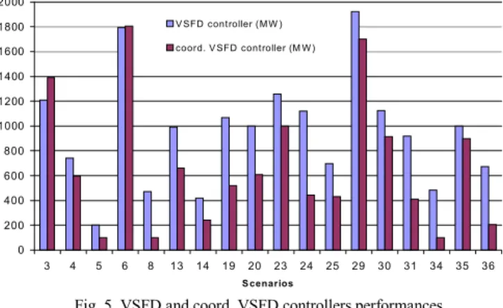
Figure 5 shows, in each unstable scenario, the total load shed by the coordinated and uncoordinated VSFD controllers, respectively. Both are based on the L∞ objective. As expected, the coordinated controller leads to less load shedding. The uncoordinated controller gives better results only in scenarios 3 and 6. It can be checked from Table 2 that in these two scenarios the Pi* value does not depend on the time sequence of shunt reactor trippings.
Table 4. Optimization results when using the L1 objective
Table 5. Optimization results when using the L∞objective
0 200 400 600 800 1000 1200 1400 1600 1800 2000 3 4 5 6 8 13 14 19 20 23 24 25 29 30 31 34 35 36 S cenarios V SFD controller (M W ) coord. V SFD controller (M W)
Fig. 5. VSFD and coord. VSFD controllers performances
To summarize, the coordinated controllers have better performances but require more computing time. An interesting trade-off would consist in working with uncoordinated VSVD controllers. Indeed, although they are less effective than their coordinated counterpart, they are the best among the uncoordinated schemes.
VI. CONCLUSIONS AND PERSPECTIVES
In this paper, three types of undervoltage load shedding controllers have been discussed. A methodology to optimize their parameters has been described and illustrated on a rather complex example. The VSVD controller seems to be the most appropriate among the uncoordinated schemes. They are however less effective than coordinated controllers managing both load shedding and automatic shunt reactor switching. On the other hand, the latter require to collect measurements from, and send controls to remote locations. The higher communication complexity has to be taken into account when assessing the overall protection reliability.
Obviously, several aspects remain to be investigated. We quote hereafter two of them.
From the computing time point of view, the branch-and-bound algorithm proposed in Fig. 4 can be improved by dynamically reordering the scenarios. In the case of the L∞ objective, this consists in memorizing during the optimization how many times each scenario has lead to a broken enumeration, and in dynamically ranking the different scenarios by decreasing order of the break frequency. Since the top ranked scenarios can be considered to be most constraining for the optimization, additional enumeration breakings can be expected by enumerating these scenarios first. The same kind of improvement can be done for the L1 objective.
A possible drawback of the proposed method is the risk of training set overfitting. This could be solved by considering very large training sets involving many stable and unstable scenarios. However, due to the combinatorial nature of the problem, the computing time would become prohibitive, in spite of the effectiveness of the branch-and-bound method.
An interesting trade-off between computing time, overfitting and effectiveness can be obtained by carrying out the optimization in two steps. First, all the controllers yielding an objective function below some predefined level could be identified, using a limited number of scenarios taken from the large training set. In a second step, these controllers could be tested on the remaining scenarios in order to find the design yielding the best average performance on the whole training set.
VII. REFERENCES
[1] Final report of TF 38.02.19, "System protection schemes in power networks", Tech. Rep., CIGRE, to appear in 2001.
[2] C. W. Taylor, Power System Voltage Stability, EPRI Power System Engineering series. 1994.
[3] C. Vournas and T. Van Cutsem, Voltage Stability of Electric Power Systems, Kluwer Academic Publishers, Boston, 1998.
[4] D. Hill S. Arnborg, G. Andersson and I. Hiskens, "On undervoltage load shedding in power systems", in Electric Power and Energy Systems, 1997,vol. 19, pp. 141-149.
[5] C. W. Taylor, "Concepts of undervoltage load shedding for voltage stability," IEEE Trans. on Power Delivery, vol. 7, pp. 480-488, 1992. [6] T. Van Cutsem, C. Moors, "Determination of optimal load shedding against
voltage instability", in 13th PSCC Proceedings,Trondheim, 1999, pp. 993-1000.
[7] W. Pulley Blank, W. Cook, W. Cunningham and A. Schrijver, Combinatorial Optimization, Wiley-Interscience, 1998.
[8] T. Van Cutsem, C. Moors, D. Lefebvre, "Combinatorial optimization approaches to the design of load shedding schemes against voltage instability", in 21th North American Power Symposium, Waterloo, Canada, 2000.