Under Memory Constraints
Antonio Sutera1 Célia Châtel2 Gilles Louppe1,3 Louis Wehenkel1 Pierre Geurts1 1University of Liège, Belgium 2Aix-Marseille University, France 3New York University, USA
Abstract
Dealing with datasets of very high dimen-sion is a major challenge in machine learn-ing. In this paper, we consider the problem of feature selection in applications where the memory is not large enough to contain all fea-tures. In this setting, we propose a novel tree-based feature selection approach that builds a sequence of randomized trees on small sub-samples of variables mixing both variables al-ready identified as relevant by previous mod-els and variables randomly selected among the other variables. As our main contribu-tion, we provide an in-depth theoretical anal-ysis of this method in infinite sample setting. In particular, we study its soundness with re-spect to common definitions of feature rele-vance and its convergence speed under vari-ous variable dependance scenarios. We also provide some preliminary empirical results highlighting the potential of the approach.
1
Motivation
We consider supervised learning and more specifically feature selection in applications where the memory is not large enough to contain all data. Such memory constraints can be due either to the large volume of available training data or to physical limits of the sys-tem on which training is performed (eg., mobile de-vices). A straightforward, but often efficient, way to handle such memory constraint is to build and aver-age an ensemble of models, each trained on only a random subset of samples and/or features that can fit into memory. Such simple ensemble approaches have the advantage to be applicable to any batch learning
Proceedings of the 21st International Conference on
Ar-tificial Intelligence and Statistics (AISTATS) 2018, Lan-zarote, Spain. PMLR: Volume 84. Copyright 2018 by the author(s).
algorithm, considered as a black-box, and they have been shown empirically to be very effective in terms of predictive performance, in particular when combined with trees, and even when samples and/or features are selected uniformly at random [see, eg., Chawla et al., 2004, Louppe and Geurts, 2012]. Independently of any considerations about memory constraints, feature sub-sampling has been shown in several works to be a very effective way to introduce randomization when build-ing ensembles of models [Ho, 1998, Kuncheva et al., 2010]. The idea of feature subsampling has also been investigated for feature selection, where several au-thors have proposed to repeatedly apply a multivari-ate feature selection technique on random subsets of features and then to aggregate the results obtained on these subsets [see, eg., Dramiński et al., 2008, Lai et al., 2006, Konukoglu and Ganz, 2014, Nguyen et al., 2015, Dramiński et al., 2016].
In this work, focusing on feature subsampling, we adopt a simplistic setting where we assume that only q input features (among p in total, with typically q p) can fit into memory. In this setting, we study ensembles of randomized decision trees trained each on a random subset of q features. In particular, we are interested in the properties of variable importance scores derived from these models and their exploita-tion to perform feature selecexploita-tion. In contrast to a purely uniform sampling of the features, we propose in Section 3 a modified sequential random subspace (SRS) approach that biases the random selection of the features at each iteration towards features already found relevant by previous models. As our main con-tribution, we perform in Section 4 an in-depth theo-retical analysis of this method in infinite sample size condition. In particular, we show that (1) this algo-rithm provides some interesting asymptotic guarantees to find all (strongly) relevant variables, (2) that ac-cumulating previously found variables can reduce the number of trees needed to find relevant variables by several orders of magnitudes with respect to the stan-dard random subspace method in some scenarios, and (3) that these scenarios are relevant for a large class of
(PC1) distributions. As an important additional con-tribution, our analysis also sheds some new light on both the popular random subspace and random forests methods that are special cases of the SRS algorithm. Finally, Section 5 presents some preliminary empirical results on several artificial and real datasets.
2
Background
This section gives the necessary background about fea-ture selection and random forests.
2.1 Feature relevance and feature selection
Let us denote by V the set of input variables, with |V | = p, and by Y the output. Feature selection is concerned about the identification in V of the (most) relevant variables. A common definition of relevance is as follows [Kohavi and John, 1997]:
Definition 1. A variable X ∈ V is relevant iff there exists a subset B ⊂ V such that X ⊥6 ⊥ Y |B. A variable is called irrelevant if it is not relevant.
Relevant variables can be further divided into two cat-egories [Kohavi and John, 1997]:
Definition 2. A variable X is strongly relevant iff Y ⊥6 ⊥ X|V \ {X}. A variable X is weakly relevant if it is relevant but not strongly relevant.
Strongly relevant variables thus convey information about the output that no other variable (or combi-nation of variables) in V conveys.
The problem of feature selection usually can take two flavors [Nilsson et al., 2007]:
All-relevant problem: finding all relevant features. Minimal optimal problem: finding a subset M ⊆ V such that Y ⊥⊥ V \ M |M and such that no proper sub-set of M satisfies this property. A subsub-set M solution to the minimal optimal problem is called a Markov boundary (of Y with respect to V ).
A Markov boundary always contains all strongly rel-evant variables and potentially some weakly relrel-evant ones. In general, the minimal optimal problem does not have a unique solution. For strictly positive dis-tributions2 however, the Markov boundary M of Y is
unique and a feature X belongs to M iff X is strongly relevant [Nilsson et al., 2007]. In this case, the solution to the minimal optimal problem is thus the set of all strongly relevant variables.
1
Defined in Section 4.2
2
Following [Nilsson et al., 2007], we will define a strictly positive distribution P over V ∪ {Y } as a distribution such that P (V = v) > 0 for all possible values v of the variables in V .
In what follows, we will need to qualify relevant vari-ables according to their degree:
Definition 3. The degree of a relevant variable X, denoted deg(X), is defined as the minimal size of a subset B ⊆ V such that Y ⊥6 ⊥ X|B.
Relevant variables X of degree 0, i.e. such that Y ⊥6 ⊥ X unconditionally, will be called marginally relevant. We will say that a subset B such that Y ⊥6 ⊥ X|B is minimal if there is no proper subset B0 ⊆ B such that Y ⊥6 ⊥ X|B0. The following two propositions give a
characterization of these minimal subsets.
Proposition 1. A minimal subset B such that Y ⊥6 ⊥ X|B for a relevant variable X contains only relevant variables.
Proof. Let us assume that B contains an irrelevant variable Xi. Let us denote by B−ithe subset B \{Xi}.
Since Xi is irrelevant, we have Y ⊥⊥ Xi|B−i∪ {X}.
Given that B is minimal we furthermore have Y ⊥⊥ X|B−i where B−i= B \ {Xi}. By using the
contrac-tion property of any probability distribucontrac-tion [Nilsson et al., 2007], one can then conclude from these two in-dependences that Y ⊥⊥ {X, Xi}|B−iand, by using the
weak union property, that Y ⊥⊥ X|B, which proves the theorem by contradiction.
Proposition 2. Let B denote a minimal subset such that Y ⊥6 ⊥ X|B for a relevant variable X. For all X0∈ B, deg(X0) ≤ |B|.
Proof. If we reduce the set of features V to a new set V0 = B ∪ {X}, X will remain relevant, as well as all features in B, given Proposition 1. So, for any feature X0 in B, there exists a subset B0 = B ∪ {X} \ X0 such that Y ⊥6 ⊥ X0|B0 and the degree of X0 is therefore
≤ |B|.
These two propositions show that a minimal condition-ing B that makes a variable dependent on the output is composed of only relevant variables whose degrees are all smaller than or equal to the size of B. We will provide in Section 4.2 a more stringent characteriza-tion of variables in minimum condicharacteriza-tionings in the case of a specific class of distributions.
2.2 Tree-based variable importances
A decision tree [Breiman et al., 1984] represents an input-output model with a tree structure, where each interior node is labeled with a test based on some input variable and each leaf node is labeled with a value of the output. The tree is typically grown using a recur-sive procedure which identifies at each node t the split
s that maximizes the mean decrease of some node im-purity measure (e.g., Shannon entropy in classification and variance in regression).
Typically, decision trees suffer from a high variance that can be very efficiently reduced by building in-stead an ensemble of randomized trees and aggre-gating their predictions. Several techniques have been proposed in the literature to grow randomized trees. For example, bagging [Breiman, 1996] builds each tree with the classical algorithm from a bootstrap sample from the original learning sample. Ho [1998]’s ran-dom subspace method grows each tree from a subset of the features of size q ≤ p randomly drawn from V . Breiman [2001]’s Random Forests combine bag-ging with a local random selection of K(≤ p) variables at each node from which to identify the best split. Given an ensemble of trees, several methods have been proposed to evaluate the importance of the vari-ables for predicting the output [Breiman et al., 1984, Breiman, 2001]. We will focus here on one particular measure called the mean decrease impurity (MDI) im-portance for which some theoretical characterization has been proposed in [Louppe et al., 2013]. This mea-sure adds up the weighted impurity decreases over all nodes t in a tree T where the variable X to score is used to split and then averages this quantity over all trees in the ensemble, i.e.:
Imp(X) = 1 NT X T X t∈T :v(st)=X p(t)∆i(st, t), (1)
with ∆i(st, t) = i(t) −
p(tL)
p(t) i(tL) − p(tR)
p(t) i(tR) where i is the impurity measure, p(t) is the proportion of samples reaching node t, v(st) is the variable used
in the split stat node t, and tLand tRare the left and
right successors of t after the split.
Louppe et al. [2013] derived several interesting prop-erties of this measure under the assumption that all variables are discrete and that splits on these variables are multi-way (i.e., each potential value of the splitting variable is associated with one successor of the node to split). In particular, they obtained the following result in asymptotic sample and ensemble size conditions: Theorem 1. X ∈ V is irrelevant to Y with respect to V if and only if its infinite sample importance as computed with an infinite ensemble of fully developed totally randomized trees built on V for Y is 0 (Theorem 3 in [Louppe et al., 2013]).
Totally randomized trees are trees obtained by set-ting Random Forests randomization parameter K to 1. This result shows that MDI importance derived from trees grown with K = 1 is asymptotically consis-tent with the definition of variable relevance given in
Algorithm 1 Sequential Random Subspace algorithm
Inputs:
Data: Y the output and V , the set of all input variables (of size p).
Algorithm: q, the subspace size, and T the number of it-erations, α ∈ [0, 1], the percentage of memory devoted to previously found features.
Tree: K, the tree randomization parameter
Output: An ensemble of T trees and a subset F of fea-tures
Algorithm: 1. F = ∅
2. Repeat T times:
(a) Let Q = R ∪ C, with R a subset of min{bαqc, |F |} features randomly picked in F without replacement and C a subset of q−|R| features randomly selected in V \ R.
(b) Build a decision tree T from Q using randomiza-tion parameter K.
(c) Add to F all features from Q that get an impor-tance greater than zero in T .
the previous section. In Section 4.1, we will actually extend this result to values of K greater than 1.
3
Sequential random subspace
In this paper, we consider a simplistic memory-constrained setting where it is assumed that only q input features can fit into memory at once, with typi-cally q small with respect to p. Under this hypoth-esis, Algorithm 1 describes the proposed sequential random subspace (SRS) algorithm to build an ensem-ble of randomized trees, which generalizes the Ran-dom Subspace (RS) method [Ho, 1998]. The idea of this method is to bias the random selection of the fea-tures at each iteration towards feafea-tures that have al-ready been found relevant by the previous trees. A parameter α is introduced that controls the degree of accumulation of previously identified features. When α = 0, SRS reduces to the standard RS method. When α = 1, all previously found features are kept while when α < 1, some room in memory is left for randomly picked features, which ensures some permanent explo-ration of the feature space. Further randomization is introduced in the tree building step through the pa-rameter K ∈ [1, q], ie. the number of variables sampled at each tree node for splitting. Variable importance is assumed to be the MDI importance. This algorithm returns both an ensemble of trees and a subset F of variables, those that get an importance (significantly) greater than 0 in at least one tree of the ensemble. Importance scores for the variables can furthermore be derived from the final ensemble using (1). In what follows, we will denote by Fq,TK,α and ImpK,αq,T (X) resp.
the set of features and the importance of feature X obtained from an ensemble grown with SRS with pa-rameters K, α, q and T .
The modification of the RS algorithm is actually mo-tivated by Propositions 1 and 2, stating that the rele-vance of high degree features can be determined only when they are analysed jointly with other relevant fea-tures of equal or lower degree. From this result, one can thus expect that accumulating previously found features will fasten the discovery of higher degree fea-tures on which they depend through some snowball effect. We confirm and quantify this effect in the next section.
Note that the SRS method can also be motivated from the perspective of accuracy. When q p and the number of relevant features r is also much smaller than the total number of features p (r p), many trees with standard RS are grown from subsets of features that contain only very few, if any, relevant features and are thus expected not to be better than random guessing Kuncheva et al. [2010]. In such setting, RS ensembles are thus expected not to be very accurate. Example 1. With p = 10000, r = 10 and q = 50, the proportion of trees in a RS ensemble grown from only irrelevant variables is Cp−rq /Cpq= 0.95.
With SRS (and α > 0), we ensure that more and more relevant variables are given to the tree growing algo-rithm as iterations proceed and therefore we reduce the chance to include totally useless trees in the ensemble. In finite settings however, there is a potential risk of overfitting when accumulating the variables. The pa-rameter α thus controls a new bias-variance tradeoff and should be tuned appropriately. We will study the impact of SRS on accuracy empirically in Section 5.
4
Theoretical analysis
In this section, we carry out a theoretical analysis of the proposed method when seen as a feature selection technique. This analysis is performed in asymptotic sample size condition, assuming that all features, in-cluding the output, are discrete, and using Shannon entropy as the impurity measure. We proceed in two steps. First, we study the soundness of the algorithm, ie., its capacity to retrieve the relevant variables when the number of trees is infinite. Second, we study its convergence properties, ie. the number of trees needed to retrieve all relevant variables in different scenarios.
4.1 Soundness
Our goal in this section is to characterize the sets of features Fq,∞K,αthat are identified by the SRS algorithm,
depending on the value of its parameters q, α, and K, in an asymptotic setting, ie. assuming an infinite sample size and an infinite forest (T = ∞). Note that in asymptotic setting, a variable is relevant as soon as its importance in one of the trees is strictly greater than zero and we thus have the following equivalence for all variables X ∈ V :
X ∈ Fq,∞K,α ⇔ ImpK,αq,∞(X) > 0
Furthermore, in infinite sample size setting, irrelevant variables always get a zero importance and thus, what-ever the parameters, we have the following property:
X ∈ V irrelevant ⇒ X /∈ FK,α
q,∞ (and Imp K,α
q,∞(X) = 0).
The method parameters thus only affect the number and nature of the relevant variables that can be found. Denoting by r (≤ p) the number of relevant variables, we will analyse separately the case r ≤ q (all relevant variables can fit into memory) and the case r > q (all relevant variables can not fit into memory).
All relevant variables can fit into memory (r ≤ q). Let us first consider the case of the RS method (α = 0). In this case, Louppe et al. [2013] have shown the following asymptotic formula for the importances computed with totally randomized trees (K = 1):
Imp1,0q,∞(X) = q−1 X k=0 1 Ck p X B∈Pk(V−m) I(X; Y |B), (2)
where Pk(V−m) is the set of subsets of V−m = V \
{xm} of cardinality k. Given that all terms are
posi-tive, this sum will be strictly greater than zero if and only if there exists a subset B ⊆ V of size at most q −1 such that Y ⊥6 ⊥X|B (⇔ I(X; Y |B) > 0), or equivalently if deg(X) < q. When α = 0, RS with K = 1 will thus find all and only the relevant variables of degree at most q − 1. Given Proposition 1, the degree of a vari-able X can not be larger than r − 1 and thus as soon as r ≤ q, we have the guarantee that RS with K = 1 will find all and only the relevant variables. Actually, this result remains valid when α > 0. Indeed, asymp-totically, only relevant variables will be selected in the F subset by SRS and given that all relevant variables can fit into memory, cumulating them will not impact the ability of SRS to explore all conditioning subsets B composed of relevant variables. We thus have:
Proposition 3. ∀α, if r ≤ q: X ∈
F1,α
q,∞ iff X is relevant.
In the case of non-totally randomized trees (K > 1), we lose the guarantee to find all relevant variables even when r ≤ q. Indeed, there is potentially a masking ef-fect due to K > 1 that might prevent the conditioning
needed for a given variable to be relevant to appear in a tree branch. However, we have the following general result:
Theorem 2. ∀α, K, if r ≤ q: X strongly relevant ⇒ X ∈ Fq,∞K,α
Proof. See Appendix A.
There is thus no masking effect possible for the strongly relevant features when K > 1 as soon as the number of relevant features is lower than q. For a given K, the features found by SRS will thus include all strongly relevant variables and some (when K > 1) or all (when K = 1) weakly relevant ones. It is easy to show that increasing K can only decrease the number of weakly relevant variables found. Using K = 1 will thus provide a solution for the all-relevant problem, while increasing K will provide a better and better ap-proximation of the minimal-optimal problem in the case of strictly positive distributions (see Section 2.1). Interestingly, Theorem 2 remains true when q = p, ie., when forests are grown without any feature sampling. It thus extends Theorem 1 from [Louppe et al., 2013] for arbitrary K in the case of standard random forests.
All relevant variables can not fit into memory (r > q). When all relevant variables can not fit into memory, we do not have the guarantee anymore to explore all minimal conditionings required to find all (strongly or not) relevant variables, whatever the val-ues of K and α. When α = 0, we have the guaran-tee however to identify the relevant variables of degree strictly lower than q. When α > 1, some space in memory will be devoted to previously found variables that will introduce some further masking effect. We nevertheless have the following general results (with-out proof): Proposition 4. ∀X : X relevant and deg(X) < (1 − α)q ⇒ X ∈ F1,α q,∞. Proposition 5.
∀K, X : X strongly relevant and deg(X) < (1 − α)q ⇒ X ∈ Fq,∞K,α.
In these propositions, (1 − α)q is simply the amount of memory that always remains available for the explo-ration of variables not yet found relevant.
Discussion. Results in this section show that SRS is a sound approach for feature selection as soon as
either the memory is large enough to contain all rel-evant variables or the degree of the relrel-evant variables is not too high. In this latter case, the approach will be able to detect all strongly relevant variables what-ever its parameters (K and α) and the total number of features p. Of course, these parameters will have a potentially strong influence on the number of trees needed to reach convergence (see the next section) and the performance in finite setting.
4.2 Convergence
Results in the previous section show that accumulat-ing relevant variables has no impact on the capacity at finding relevant variables asymptotically (when r ≤ q). It has however a potentially strong impact on the con-vergence speed of the algorithm, as measured for ex-ample by the expected number of trees needed to find all relevant variables. Indeed, when α = 0 and q p, the number of iterations/trees needed to find relevant variables of high degree can be huge as finding them requires to sample them together with all features in their conditioning. Given Proposition 2, we know that a minimum subset B such that X ⊥6 ⊥ Y |B for a rele-vant variable X contains only relerele-vant variables. This suggests that accumulating previously found relevant features can improve significantly the convergence, as each time one relevant variable is found it increases the chance to find a relevant variable of higher degree that depends on it. In what follows, we will quantify the effect of accumulation on convergence speed in differ-ent best-case and worst-case scenarios and under some simplifications of the tree building procedure. We will conclude by a theorem highlighting the interest of the SRS method in the general class of PC distributions.
Scenarios and assumptions. The convergence speed is in general very much dependent on the data distribution. We will study here the following three specific scenarios (where features {X1, . . . , Xr} are the
only relevant features):
• Chaining: The only and minimal conditioning that makes variable Xi relevant is {X1, . . . , Xi−1} (for
i = 1, . . . , r). We thus have deg(Xi) = i − 1. This
scenario should correspond to the most favorable sit-uation for the SRS algorithm.
• Clique: The only and minimal condi-tioning that makes variable Xi relevant is
{X1, . . . , Xi−1, Xi+1, . . . , Xr} (for i = 1, . . . , r). We
thus have deg(Xi) = r − 1 for all i. This is a rather
defavorable case for both RS and SRS since finding a relevant variable implies to draw all of them at the same iteration.
• Marginal-only: All variables are marginally rel-evant. We will furthermore make the assumption
that these variables are all strongly relevant. They can not be masked mutually. This scenario is the most defavorable case for SRS (versus RS) since ac-cumulating relevant variables is totally useless to find the other relevant variables and it should ac-tually slow down the convergence as it will reduce the amount of memory left for exploration.
In Appendix B.2, we provide explicit formulation of the expected number of iterations needed to find all r relevant features in the chaining and clique scenarios both when α = 0 (RS) and α = 1 (SRS). In Appendix B.3, we provide order 1 Markov chains that model the evolution through the iterations of the number of vari-ables found in the three scenarios when α = 0 and α = 1. These chains can be used to compute numeri-cally the expected number of relevant variables found through the iterations (and in the case of the marginal-only setting, the expected number of iterations to find all variables). These derivations are obtained assum-ing r ≤ q, K = q, and under additional simplifyassum-ing assumptions detailed in Appendix B.1.
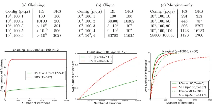
Results and discussion. Tables 1a, 1b, and 1c show the expected number of iterations needed to find all relevant variables for various configurations of the parameters p, q, and r, in the three scenarios. Figure 1 plots the expected number of variables found at each iteration both for RS and SRS in the three scenarios for some particular values of the parameters.
From these results, we can draw several conclusions. In all cases, expected times (ie., number of iter-ations/trees to find all relevant variables) depend mostly on the ratio qp, not on absolute values of q and p. The larger this ratio, the faster the convergence. Parameter r has a strong impact on convergence speed in all three scenarios.
The most impressive improvements with SRS are ob-tained in the chaining hypothesis, where convergence is improved by several orders of magnitude (Table 1a and Figure 1a) . At fixed p and q, the time needed by RS indeed grows exponentially with r (' (pq)r if r q), while time grows linearly with r for the SRS method (' rpq if r q) (see Eq. (1) and (3) in Ap-pendix B.2).
In the case of cliques, both RS and SRS need many iterations to find all features from the clique (see Table 1b and Figure 1b). SRS goes faster than RS but the improvement is not as important as in the chaining scenario. This can be explained by the fact that SRS can only improve the speed when the first feature of the clique has been found. Since the number of iterations needed to find the r features from the clique for RS is close to r times the number of iterations needed to
find one feature from the clique, SRS can only decrease at best the number of iterations by approximately a factor r (see Eq. (6) and (7) in Appendix B.2). In the marginal-only setting, SRS is actually slower than RS because cumulating the variables leaves less space in memory for exploration. The decrease of com-puting times is however contained when r is not too close to q (see Table 1c and Figure 1c).
Since we can obtain very significant improvement in the case of the chaining and clique scenarios and we only increase moderately the number of iterations in the marginal-only scenario (when r is not too close from q), we can reasonably expect improvement in gen-eral settings that mix these scenarios.
PC distributions and chaining. Chaining is the most interesting scenario in terms of convergence im-provement through variable accumulation. In this sce-nario, SRS makes it possible to find high degree rele-vant variables with a reasonable amount of trees, when finding these variables would be mostly untractable for RS. We provide below two theorems that show the practical relevance of this scenario in the specific case of PC distributions.
A PC distribution is defined as a strictly positive (P) distribution that satisfies the composition (C) prop-erty stated as follows [Nilsson et al., 2007]:
Property 1. For any disjoint sets of variables R, S, T, U ⊆ V ∪ {Y }:
S ⊥⊥ T |R and S ⊥⊥ U |R ⇒ S ⊥⊥ T ∪ U |R.
The composition property prevents the occurence of cliques and is preserved under marginalization. PC ac-tually represents a large class of distributions that en-compasses for example jointly Gaussian distributions and DAG-faithful distributions [Nilsson et al., 2007]. The composition property allows to make Proposition 2 more stringent in the case of PC:
Proposition 6. Let B denote a minimal subset B such that Y ⊥6 ⊥ X|B for a relevant variable X. If the distribution P over V ∪{Y } is PC, then for all X0 ∈ B, deg(X0) < |B|.
Proof. Proposition 2 proves that the degree of all fea-tures in B is ≤ |B| in the general case. Let us assume that there exists a feature X0 ∈ B of degree |B| in the case of PC distribution. Since this property re-main true when the set of features V is reduced to a subset V0 = B ∪ {X}, the minimal B0 of X0 can only be (B \ {Xi}) ∪ {X}. We thus have the following two
properties:
Table 1: Expected number of iterations needed to find all relevant variables for various configurations of param-eters p, q and r with RS (α = 0) and SRS (α = 1) in the three scenarios.
(a) Chaining. Config (p,q,r) RS SRS 104, 100, 1 100 100 104, 100, 2 10100 200 104, 100, 3 > 106 301 104, 100, 5 > 1010 506 105, 100, 3 > 109 3028 (b) Clique. Config (p,q,r) RS SRS 104, 100, 1 100 100 104, 100, 2 30300 10302 104, 100, 3 5 · 106 106 104, 100, 4 9 · 108 108 104, 103, 4 83785 11635 (c) Marginal-only. Config (p,q,r) RS SRS 104, 100, 10 291 312 104, 100, 50 448 757 104, 100, 90 506 2797 104, 100, 100 1123 16187 25000, 100, 50 1123 1900 r r r
Figure 1: Evolution of the number of selected features in the different scenarios.
Y ⊥⊥ X0|B0\ {X},
because B and B0are minimal. Together, by the com-position property, they should imply that
Y ⊥⊥ {X, Xi}|B \ {Xi},
which implies, by weak union: Y ⊥⊥ X|B, which con-tradicts the hypothesis.
In addition, one has the following result:
Theorem 3. For any PC distribution, let us as-sume that there exists a non empty minimal subset B = {X1, . . . , Xk} ⊂ V \ {X} of size k such that
X ⊥6 ⊥ Y |B for a relevant variable X. Then, variables X1to Xk can be ordered into a sequence {X10, . . . , Xk0}
such that deg(Xi0) < i for all i = 1, . . . , k.
Proof. Let us denote by {X10, X20, . . . , Xk0} the
vari-ables in B ordered according to their degree, ie., deg(Xi0) ≤ deg(Xi+10 ), for i = 1, . . . , k − 1. Let us show that deg(Xi0) < i for all i = 1, . . . , k. If this property is not true, then there exists at least one Xi0 ∈ B such that deg(Xi0) ≥ i. Let us denote by l the largest i such that deg(Xi) ≥ i. Using a similar argument as in
the proof of Proposition 6, there exists some minimal subset B0 ⊆ B \ {Xl} such that Y ⊥6 ⊥ Xl|B0. Given
that deg(Xl) ≥ l, this subset B should contain l
vari-ables or more from B \ {Xl}. It thus contains at least
one variable Xm with l < m ≤ k, and this variable is
such that deg(Xm) < m. Given Proposition 6, if B0
is minimal and contains Xm, then for a PC
distribu-tion, deg(Xm) should be strictly smaller than |B0| ≥ l,
which contradicts the fact that Xm is after Xl in the
ordering and proves the theorem.
This theorem shows that, with PC distributions, for all relevant variables of degree k, the k variables in its minimal conditioning form a chain of variables of increasing degrees (at worst). For PC distribution, SRS is thus guaranteed to find all relevant variables with a number of iterations that grows almost only linearly with the maximum degree of relevant variables (see Eq.3 in Appendix B.2), while RS would be unable to find relevant variables of even small degree.
5
Experiments
Although our main contribution is the theoretical anal-ysis in asymptotic setting of the previous section, we present here a few preliminary experiments in finite setting as a first illustration of the potential of the method. One of the main difficulties to implement the SRS algorithm as presented in Algorithm 1 is step 2(c) that decides which variable should be incorporated in F at each iteration. In infinite sample size setting, a variable with a non-zero importance in a single tree is guaranteed to be truly relevant. Mutual informa-tions estimated from finite samples however will always be greater than 0 even for irrelevant variables. One should thus replace step 2(c) by some statistical
sig-0 2000 4000 6000 8000 10000 Iterations 0.0 0.1 0.2 0.3 0.4 F1-measure alpha=0.0 alpha=0.5 alpha=1.0
(a) SRS with q = 0.05 × p on a dataset with p = 50000 features and r = 20 relevant features.
0 2000 4000 6000 8000 10000 Iterations 0.0 0.1 0.2 0.3 0.4 0.5 F1-measure alpha=0.0 alpha=0.5 alpha=1.0
(b) SRS with q = 0.005 × p on a dataset with p = 50000 features and r = 20 relevant features.
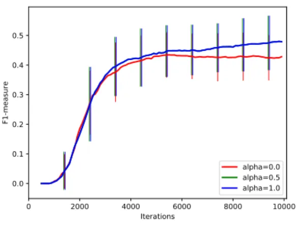
Figure 2: Evolution of the evaluation of the feature subset found by RS and SRS using the F1-measure computed with respect to relevant features. A higher value means that more relevant features have been found. This experiment was computed on an artificial dataset (similar to madelon) of 50000 features with 20 relevant features and for two sizes of memory.
nificance tests to avoid the accumulation of irrelevant variables that would jeopardize the convergence of the algorithm. In our experiments here, we use a random probe (ie., an artificially created irrelevant variable) to derive a statistical measure assessing the relevance of a variable [Stoppiglia et al., 2003]. Details about this test are given in Appendix C.
Figure 2 evaluates the feature selection ability of SRS for three values of α (including α = 0) and two mem-ory sizes (250 and 2500) on an artificial dataset with 50000 features, among which only 20 are relevant (see Appendix C for more details). The two plots show the evolution of the F1-score comparing the selected fea-tures (in F ) with the truly relevant ones as a function of the number of iterations. As expected, SRS (α > 0) is able to find better feature subsets than RS (α = 0)
for both memory sizes and both values of α > 0. Additional results are provided in Appendix C that compare the accuracy of ensembles grown with SRS for different values of α and on 13 classification problems. These comparisons clearly show that accumulating the relevant variables is beneficial most of the time (eg., SRS with α = 0.5 is significantly better than RS on 7 datasets, comparable on 5, and significantly worse on only 1). Interestingly, SRS ensembles with α = 0.5 are also most of the time significantly better than ensembles of trees grown without memory constraint (see Appendix C for more details).
6
Conclusions and future work
Our main contribution is a theoretical analysis of the SRS (and RS) methods in infinite sample setting. This analysis showed that both methods provide some guar-antees to identify all relevant (or all strongly relevant) variables as soon as the number of relevant variables or their degree is not too high with respect to the memory size. Compared to RS, SRS can reduce very strongly the number of iterations needed to find high degree variables in particular in the case of PC distributions. We believe that our results shed some new light on random subspace methods for feature selection in gen-eral as well as on tree-based methods, which should help designing better feature selection procedures. Some preliminary experiments were provided that sup-port the theoretical analysis, but more work is clearly needed to evaluate the approach empirically. We be-lieve that the statistical test used to decide which fea-ture to include in the relevant set should be improved with respect to our first implementation based on a random probe. Other procedures have been proposed to measure the statistical significance of tree-based variable importances scores that could be adapted and evaluated in our context [eg., Janitza et al., 2016]. The SRS sampling scheme could be analysed theoretically but it is admittedly very straightforward. It would be interesting to investigate, both theoretically and em-pirically, other biased sampling schemes, such as for example softer selection procedures that would sample features proportionally to their current importance. Note that biased feature sampling schemes have been proposed in the literature with different goals, e.g., in [Inza et al., 2002] as a wrapper for feature subset se-lection or in [Amaratunga et al., 2008] to improve the accuracy of random forests. It would be interesting to analyse these methods in the light of our work. Fi-nally, relaxing the main hypotheses of our theoretical analysis would be also of great interest.
Acknowledgements
Antonio Sutera received a FRIA grant from the FNRS (Belgium) and acknowledges its financial sup-port. Computational resources have been provided by the Consortium des Equipements de Calcul Intensif (CECI), funded by the Fonds de la Recherche Scien-tifique de Belgique (F.R.S.-FNRS).
References
Nitesh Chawla, Lawrence Hall, Kevin Bowyer, and Philip Kegelmeyer. Learning ensembles from bites: A scalable and accurate approach. Journal of Ma-chine Learning Research, 5:421–451, 2004.
Gilles Louppe and Pierre Geurts. Ensembles on ran-dom patches. In Machine Learning and Knowledge Discovery in Databases, pages 346–361. Springer, 2012.
Tin Kam Ho. The random subspace method for con-structing decision forests. Pattern Analysis and Machine Intelligence, IEEE Transactions on, 20(8): 832–844, 1998.
Ludmila Kuncheva, Juan Rodríguez, Catrin Plump-ton, David Linden, and Stephen Johnston. Random subspace ensembles for fmri classification. Medi-cal Imaging, IEEE Transactions on, 29(2):531–542, 2010.
Michał Dramiński, Alvaro Rada-Iglesias, Stefan En-roth, Claes Wadelius, Jacek Koronacki, and Jan Ko-morowski. Monte carlo feature selection for super-vised classification. Bioinformatics, 24(1):110–117, 2008.
Carmen Lai, Marcel Reinders, and Lodewyk Wessels. Random subspace method for multivariate feature selection. Pattern recognition letters, 27(10):1067– 1076, 2006.
Ender Konukoglu and Melanie Ganz. Approximate false positive rate control in selection frequency for random forest. arXiv preprint arXiv:1410.2838, 2014.
Thanh-Tung Nguyen, He Zhao, Joshua Zhexue Huang, Thuy Thi Nguyen, and Mark Junjie Li. A new fea-ture sampling method in random forests for predict-ing high-dimensional data. In Advances in Knowl-edge Discovery and Data Mining, pages 459–470. Springer, 2015.
Michał Dramiński, Michał Dabrowski, Klev Diamanti, Jacek Koronacki, and Jan Komorowski. Discov-ering networks of interdependent features in high-dimensional problems. In Big Data Analysis: New Algorithms for a New Society, pages 285–304. Springer, 2016.
Ron Kohavi and George John. Wrappers for feature subset selection. Artificial intelligence, 97(1):273– 324, 1997.
Roland Nilsson, José Peña, Johan Björkegren, and Jes-per Tegnér. Consistent feature selection for pattern recognition in polynomial time. Journal of Machine Learning Research, 8:589–612, 2007.
Leo Breiman, Jerome Friedman, Richard Olshen, and Charles Stone. Classification and regression trees. 1984.
Leo Breiman. Bagging predictors. Machine learning, 24(2):123–140, 1996.
Leo Breiman. Random forests. Machine learning, 45 (1):5–32, 2001.
Gilles Louppe, Louis Wehenkel, Antonio Sutera, and Pierre Geurts. Understanding variable importances in forests of randomized trees. In Advances in neural information processing, volume 26, pages 431–439, 2013.
HervÃľ Stoppiglia, GÃľrard Dreyfus, RÃľmi Dubois, and Yacine Oussar. Ranking a random feature for variable and feature selection. Journal of Machine Learning Research, 3:1399–1414, 2003.
Silke Janitza, Ender Celik, and Anne-Laure Boulesteix. A computationally fast variable importance test for random forests for high-dimensional data. Advances in Data Analysis and Classification, pages 1–31, 2016.
Inaki Inza, Pedro Larrañaga, and Basilio Sierra. Fea-ture Subset Selection by Estimation of Distribution Algorithms, volume 2, pages 269–293. Springer, 2002.
Dhammika Amaratunga, Javier Cabrera, and Yung-Seop Lee. Enriched random forests. Bioinformatics, 24(18):2010–2014, 2008.