Intra-industry Trade and Economic Distance:
Causality Tests Using Panel Data
Frédéric Peltrault and Baptiste Venet
yJuly 2005
Abstract
In this paper, we implement Granger causalty tests using panel data as methodology perfected by Hurlin (2004, 2005) and Hurlin and Venet (2004). We consider the bilateral trade patterns of the European Union with 17 countries over the period 1976-2000. We show that for the whole sample, there are no-causal relationship whatever the lag considered. However, we …nd some causal relationship from the economic distance to the share of intra-industry trade in the sample of emerging countries and the inverse relationship in the sub-sample of developing countries.
Keywords: Economic Distance, Intra-Industry Trade; Granger Caus-ality Tests; Panel Data.
JEL classi…cation: F1; C23; C11; O16; G18; G28
EURIsCO, University Paris IX Dauphine. E-mail address: [email protected]
1
Introduction
The "new" theory of international trade gives basis for the negative rela-tionship between intra-industry trade and di¤erences in factor endowment. As synthesized by Helpman and Krugman (1985), a decrease in economic distance measured by di¤erences in per capita GDP (which is a proxy for di¤erences in factor endowment) might cause an increase in the share of intra-industry trade (IIT hereafter). Granger causality tests would be a rel-evant way to assess this causal relationship. However, time-series analysis is generally di¢ cult to implement because the size of individual series is not large enough to avoid the power de…ciencies of the pure time series tests in short sample. Moreover, Hummels and Levinsohn (1995) (HL hereafter) using panel data showed that the empirical relationship between the two variables is not easy to assess.
One possible way to get round this econometric problem is to implement Granger causality tests using panel data as suggested by Hurlin (2004, 2005) and Hurlin and Venet (2004). This is what we intend to do in this paper. We consider the bilateral trade patterns of the European Union (EU hereafter) with 17 countries over the period 1976-2000.
We show that for the whole sample, there are no-causal relationship whatever the lag considered. However, we …nd some causal relationship from the economic distance (ECOD hereafter) to the share of IIT in the sub-sample of emerging countries and the inverse relationship in the sub-sub-sample of developing countries.
Paper is organized as follows. Section 1 provides a brief theoretical background for the extensive empirical literature on trade in di¤erentiated products. Section 2 presents the econometric methodology. Data and meas-ure of di¤erences in real GDP per capita and the share of IIT are presented in section 3. Section 4 presents the results. Then we conclude in section 5.
2
Theoretical and empirical background
As suggested by Linder (1961), the volume of bilateral trade is increasing with the similarity in the demand structure. Saying di¤erently, the Linder hypothesis states that countries with similar demand structure will export and import more horizontally di¤erentiated products. To the extent that di¤erence in per capita income is a proxy for the demand structure, this leads to a negative relationship between the share of intra-industry trade (IIT) and the di¤erence in GDP per capita.
The framework summarized by Helpman and Krugman (1985) show that under monopolistic competition, intra-industry trade is negatively related to di¤erences in capital-to-labor ratio. To the extent that per capita income is a good proxy for factor composition, the model predicts a negative relationship between di¤erences in per capita income and the share of intra-industry trade. Contrary to the Linder hypothesis, per capita income is now re‡ecting the supply side of the monopolistic competition model.
Another approach is developed by Flam and Helpman (1987). It enlight-ens the central role of the income distribution in trade patterns. In each coun-try, individuals with higher income consume higher quality product. Since North has a comparative advantage in high-quality products, the North ex-ports high quality products demanded by rich southern consumers whereas the South exports low quality products demanded by poor northern con-sumers. In this modelling, the share of vertical intra-industry trade can be positively related to di¤erences in per capita GDP as long as di¤erences in GDP per capita are proxying di¤erences in relative wage.
The relationship between IIT and di¤erences in per capita GDP can be either negative or positive depending on the nature of product di¤erentiation. A greater di¤erence in per capita GDP should increase the share of horizontal industry trade (HIIT) but should decrease the share of vertical intra-industry trade (VIIT). Though the sign of the causality remains uncertain, di¤erences in per capita GPD can help us to predict the trade pattern.
Since Helpman (1987), empirical studies investigate this hypothesis based upon a general equilibrium model. Econometric methods used to test this relationship are mainly Ordinary Least Square (OLS) regressions and panel data analysis. To our knowledge, time-series analysis has never been em-ployed perhaps because the sample size is not large enough due to data availability.
Helpman (1987) provides the …rst testable hypothesis based upon a gen-eral equilibrium model which partly supports the prediction that the share of intra-industry trade is decreasing with di¤erences in per capita income. This relationship is tested on a cross section of 90 country-pairs for each year from
1970 to 1981. Helpman …nds that the coe¢ cient is negative and signi…cant from 1970 to 1976 but becomes insigni…cant after.
Hummels and Levinsohn (1995; HL hereafter) revisit Helpman (1987) us-ing panel data models includus-ing 90 country pairs over 22 years. Whereas OLS regressions support Helpman’s …nding, they emphasize a positive rela-tionship when controlling for country-speci…c …xed e¤ects. This result leaves HL rather pessimistic: “if much intra-industry trade is speci…c to country pairs, we can only be sceptical about the prospects for developing any gen-eral theory to explain it”. According to HL, the theory of monopolistic competition and international trade model should account for distance to better …t the data. Recently, Anderson and Wincoop (2004) highlights that trade costs are so large that a “170% total trade barrier is constructed below as a representative rich country ad valorem tax equivalent estimate”.
Bergstrand and Egger (2004) follow HL advice and develop a model in which trade costs play a central role. Controlling for bilateral trade costs, they found a negative relationship between the share of intra-industry trade and international di¤erences in the factor composition.
Another explanation of HL results is provided by Durkin and Krygier (2000). Following Flam and Helpman (1987), they argue that a positive relationship between di¤erences in per capita income and the share of intra-industry trade is consistent with trade in vertically di¤erentiated products. Trade ‡ows are broken down into two categories, HIT and VIT, using the techniques applied by Greenaway et al. (1994)1. Unit values are used as a
proxy for quality so di¤erences in unit values reveal di¤erences in quality. Then, intra-industry trade is horizontal (vertical) when export and import unit values di¤er by less (more) than 25% for example. As predicted by the theory, Durkin and Krygier …nd a positive relationship between VIIT and di¤erences in per capita income and a negative relationship when HIIT is concerned.
3
Econometric methodology
In this paper, we use a methodology which was perfected by Hurlin (2004, 2005) and Hurlin and Venet (2004). This latter is based on a test of the Granger (1969) non causality hypothesis in a heterogeneous panel model. One of the main advantage of such a method is that it is possible to test the relationship between intra-industry trade, measured by the Grubel & Lloyd index (GLI hereafter) and di¤erences (related to EU) in real GDP per capita
1Another technique is developed by Abd-El-Rhaman (1986) and Fontagné and
(hereafter ECOD) without considering the same dynamic model for all the countries of the sample. It also permits to get round the power de…ciencies of the pure time series based tests of non-causality in short sample.
The structure of the econometric test is similar to those used in the lit-erature devoted to the panel unit tests. Under the null hypothesis, there is no causal relationship from x to y for all the countries of the panel. This hypothesis is called by Hurlin (2004, 2005) and Hurlin and Venet (2004) the "Homogeneous Non Causality" (HNC) hypothesis. Under the alternative hypothesis, there exists a causal relationships from x to y for at least one country of the sample.
This approach is similar to that used by Im, Pesaran and Shin (2003) to test the unit root hypothesis in panel data. The statistic of test is simply de…ned as the cross-sectional average of individual Wald statistics de…ned to test the Granger non Causality hypothesis for each country (Hurlin, 2004).
Let us consider two covariance stationary variables, denoted x and y; observed on T periods and on N countries. For each individual i = 1; ::; N; at time t = 1; ::; T; we have the following heterogeneous autoregressive model:
y = +X y +X x + " (1)
with = ; :::; 0. Individual e¤ects are assumed to be …xed. We assume that the lag-order K is common. The autoregressive parameters and the regression coe¢ cients slopes di¤er across countries. However, parameters and are constant. For each cross section unit i= 1; ::; N; individual residuals " ;8t = 1; ::; T are i:i:d: 0; and are independently distributed across groups.
In this heterogeneous panel model, the Homogenous Non Causality (HNC) hypothesis (H ) is:
H : = 0 8i = 1; ::N (2)
with = ; :::; 0. Under the alternative hypothesis (H ), there is a causality relationship from x to y for at least one cross-section unit. We also allow for some, but not all, of the individual vectors to be equal to 0. We assume that there are N < N individual processes with no causality from x to y:
H : = 0 8i = 1; ::; N (3)
where N is unknown but satis…es the condition 0 N =N < 1: The struc-ture of the test is similar to the unit root test in heterogeneous panels pro-posed by Im, Pesaran and Shin (2003). If the null is accepted the variable x does not Granger cause the variable y for all the countries of the panel. On the contrary, if the HNC is rejected and if N = 0; it implies that x Granger causes y for all the countries of the panel: in this case we get an homo-genous result as far as causality is concerned. The DGP (Data Generating Process) may be not homogenous, but the causality relations are observed for all countries. On the contrary, if N > 0; then the causality relationships are heterogeneous: the DGP and the causality relationships are di¤erent according the countries of the sample.
Hurlin (2004) and Hurlin and Venet (2004) propose to use the following statistics.
For a large N and T sample:
Z = r N 2K W - K ! N (0; 1) (4) with W = 1 N X W (5)
where W is the average statistic of the individual Wald statistics (W ) for the i cross section unit associated to the individual test H : = 0.
If the realization of the standardized statistic Z is superior in absolute mean to the normal corresponding critical value for a given level of risk, the homogeneous non causality (HNC) hypothesis is rejected.
For a small T sample, Hurlin (2004, 2005) and Hurlin and Venet (2004) propose to compute an approximated standardized statistic eZ for the average Wald average statistic W of the HNC hypothesis.
e Z = p N h W - N P E(W )i q N P Var(W ) (6) where for an unbalanced panel :
1 N X E(W ) ' K X (T - 2K - 1) (T - 2K - 3) (7) 1 N X Var(W ) ' 2K X (T - 2K - 1) (T - K - 3) (T - 2K - 3) (T - 2K - 5) (8)
For a large N sample, under the HNC hypothesis, Hurlin assumes that the statistic eZ follows approximately the same distribution as the stand-ardized average Wald statistic Z .
e
Z ! N (0; 1) (9)
The test of the HNC hypothesis is built as follows. For each individual of the panel, the standard Wald statistics W associated to the individual hypo-thesis H : = 0 with 2 R is commuted. Given these N realizations, we get a realization of the average Wald statistic W : Given the formula (9) we compute the realization of the approximated standardized statistic
e
Z for the T and K values: For a large N sample, if the value of eZ is superior in absolute mean to the normal corresponding critical value for a given level of risk, the homogeneous non causality (HNC) hypothesis is rejected.
4
Data
Trade data come from the COMEXT database published by Eurostat. The data are reported in four-digit Combined Nomenclature (the four-digit Nimexe until 1987) provides some 1250 items in the classi…cation of the 4-digit “Com-bined Nomenclature”. We believe that this level of desegregation is su¢ cient to prevent spurious intra-industry trade.
We investigate the causal relationship between the bilateral trade patterns of the European Union with 17 countries and economic distance over the period 1976-2000. Three country-groups are speci…ed to take into account of the level of development: developed countries, emerging countries and developing countries (see Table 11).
Real GDP per capita and Population come from the Penn World Tables, version 6.1 by Alan Heston, Robert Summers and Bettina Aten Center for International Comparisons at the University of Pennsylvania (CICUP), Oc-tober 2002.
The share of bilateral ITT is calculated with the Grubel-Lloyd index (GLI).
The share of IIT between the European Union and country k in industry i is given by:
GLI =
2 Xmin(X ; M ) X
where X and M refer respectively to the value of the European Union’s exports and imports of commodity i to country j. GLI can take value between 0 and 1; the higher GLI is, the greater is the share of IIT in total trade.
Di¤erences in GDP per capita are denoted by ECOD which stands for economic distance.
The economic distance between the European Union (EU) and country j is given by:
ECOD = max(PCGDP ; PCGDP)
min(PCGDP ; PCGDP) (11) where PCGDP stands for the per capita GDP. ECOD takes value between 1 and 1.
5
Results
For all the samples considered, we test the homogeneous non causality hypo-thesis (HNC) from ECOD to GLI and from GLI to ECOD. In each case, we compute three statistics: the average Wald statistic W , the standardized statistic Z based on the asymptotic moments and the standardized stat-istic eZ based on the approximation of …nite sample moments. In order to assess the sensitivity of our results to the choice of the common lag-order, we compute all these statistics for one, two and three lags.
The results for the complete sample of 17 developed, emerging and devel-oping countries are reported in tables 2 and 3. When the inference is based on the asymptotic standardized statistic Z or on the approximated stand-ardized statistic eZ , the homogenous non causality (HNC) between ECOD and GLI is never rejected at a 5% signi…cant level, whatever the direction of causality and whatever the lag order. It implies that the past values of di¤erences in real GDP per capita (resp. intra-industry trade) are not useful when one intends to forecast intra-industry trade (resp. di¤erences in real GDP per capita) for the whole sample of 17 countries.
Insert tables 2 and 3
One important issue is to determine if this absence of causal relationship is a common characteristic of developed, emerging and developing countries of our sample. For that, we consider the same tests for a sub-sample of 3 de-veloped countries (Canada, Japan and USA) (tables 4 and 5), a sub-sample of 7 emerging economies (Brazil, Chile, Indonesia, South Korea, Mexico, Singa-pore and Taiwan) (tables 6 and 7) a sub-sample of 7 developing countries
(Egypt, India, Morocco, Malaysia, Philippines, Tunisia and Turkey) (tables 8 and 9).
Insert tables 4 and 5 Insert tables 8 and 9
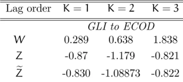
For developed countries, the conclusions are similar to those obtained in the complete sample: the homogenous non causality (HNC) between ECOD and GLI is never rejected at a 5% signi…cant level, whatever the direction of causality and whatever the lag. However, for emerging and developing countries, results are a little bit di¤erent. As far as the emerging countries sample are concerned, we can observe that the HNC hypothesis from ECOD to GLI is strongly and robustly rejected when the inference is based on the asymptotic moments properties and when a lag of 3 periods is chosen (tables 6). It implies that the past values of di¤erences in real GDP per capita are useful to forecast intra-industry trade between EU and emerging economies of that sub-sample.
Last but not least, the HNC hypothesis from GLI to ECOD is strongly and robustly rejected (table 9) for developing countries and for a 2 periods lag. It implies that the past values of GLI are useful to forecast di¤erences in real GDP per capita between EU and developing countries.
To summarize, it seems that developed countries play a major role in the whole panel since the HNC hypothesis is no longer accepted as soon as these countries are excluded from the panel.
6
Conclusion
In this paper, we examined the causal relationship between the economic distance and the share of intra-industry trade using panel data causality analysis. Our results do not support the prediction of the "new" theory of international trade since one could expected a causal relationship from ECOD to GLI at least for developed countries. However, this relationship does exist for emerging countries which trade with EU is becoming more and more important especially since the middle of the 90’s.
There are two possible ways to improve the analysis. On the one hand, It would be relevant to re-examine the causal relationship including a trade costs variable as it is recommended by HL. In fact, Bergstrand and Egger (2004) show that the e¤ect of an increase in only di¤erentiated trade costs on GLI is also sensitive to relative factor endowment di¤erences. By doing this, it would be possible to estimate the causal relationship holding constant
trade costs. On the other hand, it might be useful to break intra-industry trade down into vertical and horizontal intra-industry trade.
A
Data appendix
All GDP series can be downloaded at the following internet address: http://datacentre2.chass.utoronto.ca/pwt/alphacountries.html. The classi…cation of countries used in the paper is the following.
Insert tables 11
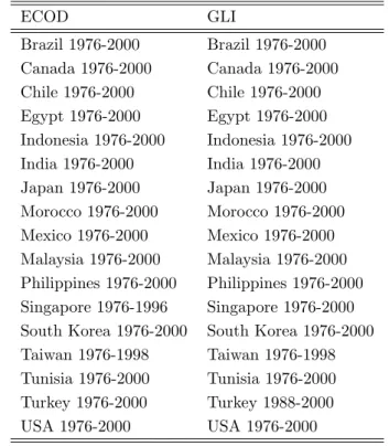
Most individual series starts in 1976 and ends in 2000. However, some of them are incomplete in the sense that they …nish earlier. This implies that panels we use are unbalanced ones. Individual samples for countries which data are incomplete are reported in the table 10.
B
Sensitivity analysis
In the two …rst tables 2 and 3, the results obtained with a panel of 17 countries over the period 1976-2000, are reported.
On tables 4 and 5, the results for the sample of 3 developed countries over the period 1976-2000 are reported.
On tables 6 and 7, the results for the sample of 7 emerging economies over the period 1976-2000 are reported.
On tables 8 and 9, the results for the sample of 7 developing countries over the period 1976-2000, are reported.
References
[1] Abd-El-Rahman, K. S. (1986). Réexamen de la dé…nition et de la mesure des échanges croisés de produits similaires entre les nations, Revue économique, 37(1), pp. 89-115.
[2] Anderson and Wincoop (2004), Trade Costs. Journal of Economic Lit-erature, 42(3), pp. 691-751.
[3] Bergstrand J.H. and P. Egger (2004).Trade Costs and Intra-Industry Trade (with), mimeo, University of Notre Dame.
[4] Durkin, John T. and Krygier, Markus (2000). Di¤erences in GDP Per Capita and the Share of Intra-industry Trade: The Role of Vertically Di¤erentiated Trade" Review of International Economics, 8, pp. 760-774, November.
[5] Flam, H. and E. Helpman (1987), “Vertical Product di¤erentiation and North-South trade”. American Economic Review, 76, pp. 810-22. [6] Fontagné, L. and M. Freudenberg (1997). Intra-industry Trade:
Meth-odological Issues Reconsidered, CEPII Working Paper, No.97-01. [7] Granger, C.W.J., (1969). Investigating causal relationd by econometric
models and cross-spectral methods. Econometrica 37, 424–438.
[8] Greenaway D., R. Hine and C. Milner (1994), Country-Speci…c Factors and the Pattern of Horizontal and Vertical Intra-Industry Trade in the UK, Weltwirtschaftliches Archiv, 130, pp. 77-100.
[9] Helpman E. (1987), Imperfect Competition and International Trade: Evidence from Fourteen Industrial Countries. Journal of the Japanese and international Economics, 1(1), pp. 62-81.
[10] Hummels D. and J. Levinsohn (1995), Monopolistic Competition and International Trade: Reconsidering the Evidence, Quarterly Journal of Economics, 110(3),pp. 799-836.
[11] Hurlin, C., (2004). Testing Granger Causality in Heterogeneous Panel Data Models with Fixed Coe¢ cients. Document de recherche LEO, [12] No. 2004-05, Université d’Orléans.
[13] Hurlin, C., (2005). Un Test Simple de l’Hypothèse de Non Causalité dans un Modèle de Panel Hétérogène. Revue Economique, forthcoming. [14] Hurlin, C. Venet, B. (2004). Financial Development and Growth : A Re-Examination using a Panel Granger Causality Test, Document de Recherche du LEO; No. 2004-18.
[15] Im, K.S., Pesaran, M.H., Shin, Y., (2003). Testing for Unit Roots in Heterogeneous Panels. Journal of Econometrics 115(1), 53–74.
[16] Linder, S.B. (1961). An Essay on Trade and Transformation, New York: Wiley and Sons.
[17] Maddala, G.S. Wu, S., (1999). A Comparative Study of Unit Root Tests with Panel Data and a New Simple Test. Oxford Bulletin of Economics and Statistics, special issue, 631–652.
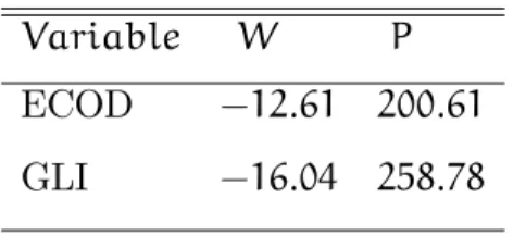
Table 1: Panel Unit Root Tests Variable W P ECOD -12:61 200:61 GLI -16:04 258:78
Notes: W denotes the standardizedIPSstatistic based on simulated approximated moments (Im, Pesaran and Shin, 2003, table 3). P de-notes the Fisher’s test statistic proposed by Maddala and Wu (1999) and on individual ADFp-values. UnderH ; P has a distribution with2N
of freedom whenT tends to in…nity andNis …xed. Correspondingp-values are in parentheses.
Table 2: Causality from di¤erences in real GDP per capita to intraindustry trade. 17 Countries Lag order K= 1 K= 2 K= 3 ECOD to GLI W 0.7999 2.178 4.093 Z -0.583 0.367 1.84 e Z -0.752 -0.151 0.665
Table 3: Causality from intraindustry trade to di¤erences in real GDP per capita. 17 countries Lag order K= 1 K= 2 K= 3 GLI to ECOD W 0.902 2.101 1.963 Z -0.285 0.209 -1.744 e Z -0.507 -0.273 -1.805
Table 4: Causality from di¤erences in real GDP per capita to intraindustry trade. 3 Developed countries
Lag order K= 1 K= 2 K= 3 ECOD to GLI W 1.798 2.422 4.124 Z 0.978 0.365 0.795 e Z 0.695 0.104 0.309
Table 5: Causality from intraindustry trade to di¤erences in real GDP per capita. 3 Developed countries
Lag order K= 1 K= 2 K= 3 GLI to ECOD W 0.289 0.638 1.838 Z -0.87 -1.179 -0.821 e Z -0.830 -1.08873 -0.822
Table 6: Causality from di¤erences in real GDP per capita to intraindustry trade. 7 emerging economies
Lag order K= 1 K= 2 K= 3 ECOD to GLI W 0.459 2.143 6.126 Z -1.01 0.189 3.377 e Z -1.005 -0.142 1.882
Table 7: Causality from intraindustry trade to di¤erences in real GDP per capita. 7 emerging economies
Lag order K= 1 K= 2 K= 3 GLI to ECOD W 0.759 1.197 1.425 Z -0.45 -1.062 -1.701 e Z -0.547 -1.09 -1.546
Table 8: Causality from di¤erences in real GDP per capita to intraindustry trade. 7 developing countries
Lag order K= 1 K= 2 K= 3 ECOD to GLI W 0.711 2.108 2.046 Z -0.539 0.143 -1.029 e Z -0.617 -0.161 -1.098
Notes: indicates rejection at 5% level.
Table 9: Causality from intraindustry trade to di¤erences in real GDP per capita. 7 developing countries
Lag order K= 1 K= 2 K= 3 GLI to ECOD W 1.307 3.632 2.555 Z 0.575 2.16 -0.479 e Z 0.303 1.394 -0.713
Table 10: Samples for incomplete individual series ECOD GLI Brazil 1976-2000 Brazil 1976-2000 Canada 1976-2000 Canada 1976-2000 Chile 1976-2000 Chile 1976-2000 Egypt 1976-2000 Egypt 1976-2000 Indonesia 1976-2000 Indonesia 1976-2000 India 1976-2000 India 1976-2000 Japan 1976-2000 Japan 1976-2000 Morocco 1976-2000 Morocco 1976-2000 Mexico 1976-2000 Mexico 1976-2000 Malaysia 1976-2000 Malaysia 1976-2000 Philippines 1976-2000 Philippines 1976-2000 Singapore 1976-1996 Singapore 1976-2000 South Korea 1976-2000 South Korea 1976-2000 Taiwan 1976-1998 Taiwan 1976-1998 Tunisia 1976-2000 Tunisia 1976-2000 Turkey 1976-2000 Turkey 1988-2000 USA 1976-2000 USA 1976-2000
Table 11: List of countries
Developed countries Emerging Economies Developing countries Canada Brazil Egypt
Japan Chile India United States Indonesia Morocco
South Korea Malaysia Mexico Philippines Singapore Tunisia Taiwan Turkey