HAL Id: pastel-01063720
https://pastel.archives-ouvertes.fr/pastel-01063720
Submitted on 12 Sep 2014
HAL is a multi-disciplinary open access archive for the deposit and dissemination of sci-entific research documents, whether they are pub-lished or not. The documents may come from teaching and research institutions in France or abroad, or from public or private research centers.
L’archive ouverte pluridisciplinaire HAL, est destinée au dépôt et à la diffusion de documents scientifiques de niveau recherche, publiés ou non, émanant des établissements d’enseignement et de recherche français ou étrangers, des laboratoires publics ou privés.
selection strategies for populations of different diversity
levels : Application in maize (Zea mays L.)
Renaud Rincent
To cite this version:
Renaud Rincent. Optimization of association genetics and genomic selection strategies for populations of different diversity levels : Application in maize (Zea mays L.). Agricultural sciences. AgroParisTech, 2014. English. �NNT : 2014AGPT0018�. �pastel-01063720�
AgroParisTech UMR de Génétique Végétale
INRA/Univ. Paris Sud/CNRS
Ferme du Moulon, 91190 Gif-sur-Yvette, France
présentée et soutenue publiquement par
Renaud RINCENT
le 11 Avril 2014
Optimization of association genetics and genomic selection strategies
for populations of different diversity levels.
Application in maize (Zea mays L.).
Doctorat ParisTech
T H È S E
pour obtenir le grade de docteur délivré par
L’Institut des Sciences et Industries
du Vivant et de l’Environnement
(AgroParisTech)
Spécialité : Sciences de la vie et santé
Directeur de thèse : Alain Charcosset
Co-encadrement de la thèse : Laurence Moreau, Milena Ouzunova, Pascal Flament, Pierre Dubreuil Travaux réalisés dans le cadre d'une convention CIFRE, avec l'aide de l'ANRT
Jury
M. John HICKEY, Docteur, Roslin Institute, Edinburgh Rapporteur
M. Gilles CHARMET, Directeur de Recherches, INRA de Clermont-Ferrand Rapporteur
M. David CAUSEUR, Professeur, Mathématiques appliquées, Agrocampus Ouest Examinateur
M. Etienne VERRIER, Professeur, AgroParisTech Examinateur
M. Pascal FLAMENT, Head of research support functions, Limagrain Co-encadrant
Mme Laurence MOREAU, Chargée de Recherches, INRA du Moulon Co-encadrante
3 - Pour ces 3 ans fermes du Moulon -
Mes remerciements vont d'abord à Alain et Laurence qui m'ont fait confiance et soutenu au cours de ces trois années. La richesse de nos échanges et de vos engagements m'ont été très précieux. C'est en bonne partie grâce à vous que j'ai pu découvrir, profiter et m'intégrer peu à peu au monde passionnant de la recherche : j'ai maintenant le doigt pris dans l'engrenage de la machine infernale, bravo vous pouvez être fier de vous ! J'espère pouvoir continuer à travailler avec vous sur de nouvelles idées... Merci également aux autres membres de GQMS de m'avoir fait confiance pour donner quelques cours aux étudiants (Julie), pour les échanges qu'on a pu avoir (Tristan, Cyril, Stéphane, Delphine). Merci Tristan (mon prof de TD de stat à Grignon !) pour tes supers cours et démos en direct, ta pédagogie, ton grand tableau et nos échanges. Merci Cyril d'avoir toujours pris le temps de m'expliquer des choses au bureau ou au champs, et pour ton initiation aux dégustations œnologiques, et merci de m'avoir fait découvrir que j'étais marié à un Nez... Merci André de m'avoir recommandé le stage chez KWS avec Dietrich, qui m'a lancé sur la voie de la génétique. Merci pour votre passion communicative, et de prendre à chaque fois plaisir à discuter avec nous, les étudiants.
Pour leur accompagnement, le temps qu'ils ont pris à m'accueillir et à m'exposer leurs problématiques, je remercie mes collègues de KWS, en particulier Milena et Thomas (vielen Dank), mes collègues de Limagrain (Pascal, Zivan, Simon, Sébastien...) et de Biogemma (Pierre et Sébastien), ainsi que Sylvie Guillaume pour son efficacité et sa gentillesse. Merci à Pascal, Milena et Sébastien d'avoir accepté de financer ma thèse. Un grand merci à tous ceux qui ont travaillé sur les expérimentations du réseau INRA (Cyril et Jacques en particulier) et de nos partenaires Allemands et Espagnols pour le très gros travail de terrain sans lequel ma thèse n'aurait pas été possible. Egalement merci à tous ceux qui ont réalisé les analyses de laboratoire (Delphine, Valérie, Fabrice...).
Je remercie John Hickey, Gilles Charmet, David Causeur, Etienne Verrier et Pascal Flament d'avoir accepté de faire partie de mon jury de thèse.
Je remercie également toute la République démocratique du Moulon pour sa très bonne ambiance collective, son ouverture d'esprit et sa richesse humaine et scientifique. L'ambiance change en permanence avec les arrivées et départs mensuels, l'évolution de la faune endémique, mais elle reste toujours très bonne. Je remercie d'abord l'équipe de choc de jeunes présents à mon arrivée: Nico, Marion, Amandine, Fabio, Pierre M, Sophie, Mathieu, Bub,
4 plus tard Mariangela, Héloïse, Margot, Telma, Aude, Sandra, les Sara, Margaux-Alison, Christophe, Adrien, Jean-Tristan, Cyril. Merci à mes collègues de bureau Mariangela (bout de choco ?) et Héloïse (bout de choco ? Ah non c'est vrai...), pour l'architecture d'intérieur, la déco et la bonne ambiance. Merci Sophie pour nos discussions et ta précieuse aide, Nicolas et Amandine pour vos conseils. Merci à Christine, Jérôme, Maud, Karin, Isabelle, Dominique, Domé, Matthieu, Philippe pour nos discussions. Merci Valérie pour ta grande cuisine et ta gentillesse. Philippe, Marlène, Xavier, Fabrice, pour les rigolades.
Je remercie les collègues de Jouy (de m'avoir laisser harceler Bananier), et notamment Hervé et Estelle pour nos échanges. Merci Estelle pour tes conseils, ton soutien et ta bonne humeur. Je remercie également toutes les personnes que j'ai croisées au cours de ma thèse et avec qui j'ai pu avoir de riches échanges : l'équipe d'Orléans (Vincent et Leopoldo en particulier), de Toulouse (Andres et Bertrand), Jose Crossa, Catherine Giauffret, Christopher Sauvage, Denis Laloë et tous les autres.
Merci aux copains pour leur amitié forte et riche, et les grands moments passés ensemble, merci Laurent, Baptiste, Anne, Anaïs, Alexis, Gildas et Schérou, Armand, David et Chloé. Je remercie tout particulièrement ma famille, sans qui tout cela n'aurait pas été possible. Vous avez toujours été présents et m'avez donné de la force dans les moments difficiles.
5
"Nous n'avons que faire d'aller trier des miracles et des difficultés étrangères : il me semble que parmi les choses que nous voyons ordinairement, il y a des étrangetés si incompréhensibles, qu'elles surpassent toute la difficulté des miracles. Quel monstre est-ce, que cette goutte de semence, de quoi nous sommes produits, porte en soi les impressions, non de la forme corporelle seulement, mais des pensements et des inclinations de nos pères. Cette goutte d'eau, où loge ce nombre infini de formes : et comme portent-elles ces ressemblances, d'un progrès si téméraire et si déréglé, que l'arrière-fils répondra à son bisaïeul, le neveu à l'oncle."
Essais de M. de Montaigne (1580). Livre II, chap. 37.
7 Major progresses have been achieved in genotyping technologies, which makes it easier to decipher the relationship between genotype and phenotype. This contributed to the understanding of the genetic architecture of traits (Genome Wide Association Studies, GWAS), and to better predictions of genetic value to improve breeding efficiency (Genomic Selection, GS). The objective of this thesis was to define efficient ways of leading these approaches. We first derived analytically the power from classical GWAS mixed model and showed that it was lower for markers with a small minimum allele frequency, a strong differentiation among population subgroups and that are strongly correlated with markers used for estimating the kinship matrix K. We considered therefore two alternative estimators of K. Simulations showed that these were as efficient as classical estimators to control false positive and provided more power. We confirmed these results on true datasets collected on two maize panels, and could increase by up to 40% the number of detected associations. These panels, genotyped with a 50k SNP-array and phenotyped for flowering and biomass traits, were used to characterize the diversity of Dent and Flint groups and detect QTLs. In GS, studies highlighted the importance of relationship between the calibration set (CS) and the predicted set on the accuracy of predictions. Considering low present genotyping cost, we proposed a sampling algorithm of the CS based on the G-BLUP model, which resulted in higher accuracies than other sampling strategies for all the traits considered. It could reach the same accuracy than a randomly sampled CS with half of the phenotyping effort.
Key words: maize, genomic selection, association mapping, power, accuracy, biomass.
RESUME
D’importants progrès ont été réalisés dans les domaines du génotypage et du séquençage, ce qui permet de mieux comprendre la relation génotype/phénotype. Il est possible d'analyser l’architecture génétique des caractères (génétique d’association, GA), ou de prédire la valeur génétique des candidats à la sélection (sélection génomique, SG). L’objectif de cette thèse était de développer des outils pour mener ces stratégies de manière optimale. Nous avons d’abord dérivé analytiquement la puissance du modèle mixte de GA, et montré que la puissance était plus faible pour les marqueurs présentant une faible diversité, une forte différentiation entre sous groupes et une forte corrélation avec les marqueurs utilisés pour estimer l’apparentement (K). Nous avons donc considéré deux estimateurs alternatifs de K. Des simulations ont montré qu'ils sont aussi efficaces que la méthode classique pour contrôler
8 corné et denté du programme Cornfed, avec une augmentation de 40% du nombre de SNP détectés. Ces panels, génotypés avec une puce 50k SNP et phénotypés pour leur précocité et leur biomasse ont permis de décrire la diversité de ces groupes et de détecter des QTL. En SG, des études ont montré l’importance de la composition du jeu de calibration sur la fiabilité des prédictions. Nous avons proposé un algorithme d’échantillonnage dérivé de la théorie du G-BLUP permettant de maximiser la fiabilité des prédictions. Par rapport à un échantillon aléatoire, il permettrait de diminuer de moitié l’effort de phénotypage pour atteindre une même fiabilité de prédiction sur les panels Cornfed.
9
Abstract ... 7
General introduction ... 13
Chapter 1 ... 25
Recovering power in association mapping panels with variable levels of linkage disequilibrium ... 27
ABSTRACT ... 28
INTRODUCTION ... 29
MATERIALS AND METHODS ... 31
Statistical models for association mapping and power evaluation ... 31
Analytical evaluation of the impact of panel characteristics on power ... 32
Kinship estimation ... 33
Simulation based evaluation of the impact of the estimation of K on false positive control and power ... 35
Genetic material and genotyping data ... 37
Specific parameterization ... 37
RESULTS ... 38
Diversity and Linkage Disequilibrium in maize panels ... 38
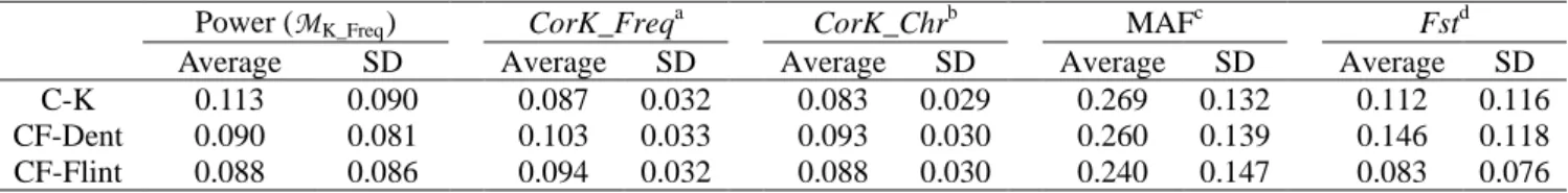
Relationship between MAF, Fst, CorK and power ... 38
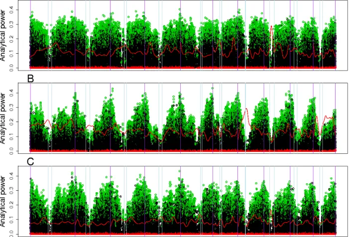
Variation of analytical power and CorK along chromosomes ... 39
Simulation based assessment of kinship estimation on false positive control and power ... 43
DISCUSSION AND CONCLUSIONS ... 46
Analytical investigation of potential power along the genome with usual model (MK_Freq) ... 46
Simulation based comparison of type I risk and power of statistical models associated with different estimations of K ... 48
Acknowledgments ... 49
LITERATURE ... 50
Chapter 2 ... 57
Dent and Flint maize diversity panels reveal important genetic potential for increasing biomass production ... 59
ABSTRACT ... 60
10
Genetic material and genotyping data ... 62
Diversity analysis ... 63
Linkage Disequilibrium (LD) ... 64
Phenotypic data ... 65
Phenotypic characterization of the genetic groups within each panel... 67
Statistical model for association mapping ... 67
RESULTS ... 68
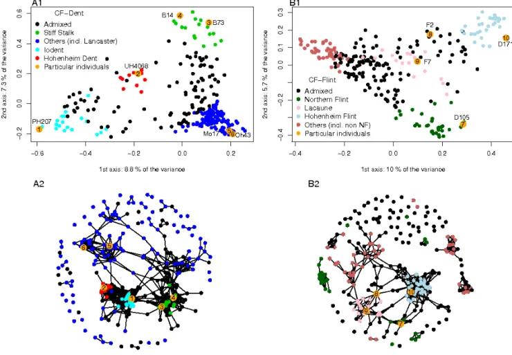
Diversity and structure analysis ... 68
Linkage disequilibrium ... 71
Phenotypic variation ... 73
Phenotypic characterization of the genetic groups within each panel... 73
Association mapping results ... 75
DISCUSSION AND CONCLUSION ... 89
Genetic Diversity organization ... 79
Trait variation within and among genetic groups ... 81
Association mapping results ... 82
Conclusions ... 83 Acknowledgments ... 84 LITERATURE ... 85 Chapter 3 ... 91 ABSTRACT ... 93 INTRODUCTION ... 93
MATERIALS AND METHODS ... 95
Genetic material ... 95
Field data ... 95
Genotyping, diversity and relationship matrix ... 95
Statistical model ... 96
Optimization criteria and CD ... 96
Optimization algorithm ... 97
Observed prediction reliability and robustness of the optimization to variation of heritability ... 97
Link between the PEV and the observed prediction error ... 98
Genetic properties of optimized calibration sets ... 98
RESULTS ... 98
11 Observed prediction reliability and robustness of the optimization to variation of
heritability ... 98
Link between the PEV and the observed prediction error ... 98
Genetic properties of optimized calibration sets ... 100
DISCUSSION ... 100
Acknowledgments ... 105
LITERATURE ... 105
General discussion ... 107
Increasing power in association mapping ... 110
Using molecular information to maximize GS efficiency: optimizing the sampling of the calibration set ... 112
Diversity analysis and association mapping in the Dent and Flint Cornfed panels ... 114
Towards an integrated approach in plant breeding ... 115
LITERATURE ... 117
APPENDICES ... 129
Appendix I: supplemental chapter 1 ... 131
Appendix II: supplemental chapter 2 ... 135
13
General introduction
15 Plant breeding appeared 9 000 to 12 000 years ago, when humans became sedentary and developed agriculture. The first plants that were cultivated for a given species accumulated alleles which facilitated the cultivation, harvest and/or use of harvested products. Note that these favorable alleles may have long existed in wild populations or appeared simultaneously through mutations. This transition from wild reproduction to cultivation occurred independently for many species in several regions of the world and is referred to as domestication. After the first steps of domestication, the process was continued by farmers to increase the value of plants for previous criteria. Both during domestication and later steps, seeds from the plants with the best agronomical characteristics were selected for the sowing of the next season. Divergence between domesticated individuals and their wild ancestors increased with time and could result in huge phenotypic variability. This is for example the case of maize (Zea mays ssp. mays), which became very different from the teosinte subspecies (ssps. parviglumis and mexicana) from which it was domesticated in Mesoamerica starting around 9000 years ago (Beadle 1939; Matsuoka et al. 2002; Doebley 2004). The selection of individuals of higher phenotypic value, called selective breeding, generated plants improved in terms of utility for humans (e.g. yield, composition, precocity), instead of maximizing fitness only as would natural selection do. Selective breeding was used for millennia, until the 20th century for maize. One main limit of this approach is that it is based on the phenotype of single plants in a particular environment. As this phenotype is the result of both genotypic and environmental factors, it does not reflect directly the genetic potential, i.e. the Genetic Value (GV). This could be conceptualized only in the early 1900s after the founding work of precursory scientists.
Gregor Mendel, considered as the founder of genetics, first understood and described the inheritance of traits influenced by few genes (qualitative traits) by studying the segregation of color and shape in peas (Mendel 1866). His work was synthesized into the famous laws of inheritance: the law of segregation and the law of independent assortment. Approximately at the same time Francis Galton developed statistical approaches (1869, 1879) to study quantitative traits (continuous traits, for example human height), laying the foundation of the biometrical school. Mendel's theory was criticized at this time, in particular because it could not explain how continuous traits are inherited, and was thought to be contradictory to the approach of Francis Galton. R. A. Fisher later proved (1918) that Mendel's laws could be extended to continuous traits by showing that the combined effect of many genes and the environment could give rise to continuous phenotypic variations. It is also in the early 20th
16 century that W. Johannsen introduced the notions of genotype and phenotype in his famous experiments on variability between and within pure lines of beans (1903). These first developments of quantitative genetics allowed the mathematical formalization of the relationship between genotype and phenotype, the phenotype being seen as a realization of a genotype in an environment. This gave birth to many concepts of applied statistics used in numerous and various fields. Evolutionary theories also developed since the mid 1800s with the concept of natural selection (see Darwin's seminal book "On the Origin of species", 1859). This concept together with gradual evolution, and Mendelian genetics were synthesized in the so called "modern evolutionary synthesis" (Huxley 1942), the most accepted paradigm in evolutionary biology, which establishes that variation has to be heritable to undergo natural selection. We now know that these variations submitted to natural selection can have different origins including genetic and epigenetic factors.
In animal and plant breeding, statistical models could then be developed to predict and compare the gain of different selection strategies (Falconer and Mackay 1996; Gallais 1990), and as a result optimize these. Genetic progress was formally decomposed into four components: genetic variability, selection intensity, generation interval, and the accuracy of the estimations of GVs. The replicated observation of a genotype in different environments, or the observations of related individuals (first statistically modeled by Henderson, 1963) allowed the distinction between the effect of the genotype (GV), the effect of the environment (micro and macro environment), and the potential interaction between the genotypic and environmental effects. The selection strategies based on GV estimates have been extensively and efficiently used in breeding. In plant breeding, the possibility to generate numerous individuals with the same genotype, through cloning or most often the production of inbred lines, allows the evaluation of the genotype in field trial networks. This was the most common approach used for phenotypic evaluation in plants until recently. In maize, which is mostly allogamous, inbred lines have poor performance because of inbreeding and are thus crossed to produce hybrids, taking advantage of heterosis (Shull 1908). Hybrid breeding in maize contributed to a huge increase in productivity, with average grain yields increasing from 1.5 to 8 t/ha between 1935 and 2000 in the USA (Troyer 2005). One limitation of these strategies mainly based on phenotypic data is that they are conducted without knowing the genes underlying the variation of the phenotypic trait (number, positions, and effects) and thus without knowing the favorable alleles that could be combined to produce an improved genotype.
17 The question is then, how to identify favorable alleles ? A first answer was obtained, again on peas, by Sax (1923), who identified an association between the size (quantitative trait) and the color (qualitative trait) of seeds. His experiment thus revealed that a local mutation (responsible for the seed color) was associated with a quantitative trait (the size of the seeds). The color can be seen here as a phenotypic marker: it directly reveals the genotype at a locus (implied in seed color), which was associated with the genotype at a locus influencing a quantitative trait (a so-called Quantitative Trait Locus or QTL, associated here with the size) through physical linkage. The law of independent assortment states that the alleles at a locus segregate independently from the alleles at another locus during meioses if they are located on different chromosomes. If not, the two loci are physically linked and are separated only if a crossover occurs between them. The probability that a recombination occurs during meioses defines the concept of genetic distance (expressed in centiMorgan, cM). As a consequence, two linked genes are more or less correlated (in Linkage Disequilibrium, LD), depending on the genetic distance that separates them. Correlation between two linked loci implies that a marker can capture (at least partially) the effect of nearby QTL(s). Phenotypic markers are however often of poor interest, because they are rare and often dominant. The development of molecular markers in the 1960s made it possible to carry out the first QTL detection experiments with 10-30 polymorphic markers within a given population. The first molecular markers were protein variants (isozymes) identified by electrophoresis. These variations have the advantage of being codominant but they are not very polymorphic and not numerous enough to cover the entire genome. In the 1980s, new approaches appeared, enabling to detect polymorphism at the DNA level, revealing polymorphism in the presence or absence of restriction sites (Restriction Fragment Length Polymorphism, RFLP), in the length of the amplified fragments (Amplified Fragment Length Polymorphism, AFLP) or in the number of copies of microsatellites (Single Sequence Repeat, SSR). This permitted the development of an increasing number of markers and the first genomewide QTL mapping approaches really started in 1988 with the seminal paper of Paterson et al.. The progress made in DNA sequencing later allowed the identification of numerous polymorphisms at the level of single nucleotides (called SNP). These SNPs rapidly became the most commonly used markers, because they can be automatically analyzed with SNP-arrays providing cheap, numerous and codominant markers. The fact that SNPs are generally biallelic, and thus less informative than SSRs, is counterbalanced by the fact that thousands to millions of SNPs are now available for many species. High throughput SNP-arrays have been developed and are extensively used in
18
human, animal and plant genetics. In maize, a 50,000 SNP-array was developed (GANAL et al.
2011) following the sequencing of B73 (ZHOU et al. 2009; WEI et al. 2009a; WEI et al.
2009b), the first maize inbred line sequenced, and the resequencing of numerous inbred lines. Technological progress in sequencing makes it now possible to genotype individuals directly by sequencing portions of their genomes. Several Genotyping By Sequencing (GBS)
strategies are now available (ELSHIRE et al. 2011).
These tools, combined with phenotypic data, offer different ways of detecting QTLs. In linkage-based QTL detection, individuals with contrasted phenotypes are crossed to produce a segregating population. In this kind of populations linkage between markers and QTLs makes it possible to detect associations between phenotypic variability and marker polymorphism. Major QTLs were detected with this approach, and the underlying gene was sometimes identified after analyzing numerous recombinant individuals in the genomic region of interest (HUANG et al. 1997; SALVI and TUBEROSA 2005; GIULIANI et al. 2005; DUCROCQ et al. 2009).
However the low diversity of the material used as parents (a significant proportion of QTLs are monomorphic), and the low resolution of the detection (often confined to a range of 10 to
30 cM, FLINT-GARCIA et al. 2003; ZHU et al. 2008) are important limits to this approach and
makes it difficult to identify the underlying genetic factor(s).These difficulties can be circumvented to some extent by increasing the number of parents and the size of the total
population (YU et al. 2008; CAVANAGH et al. 2008; BARDOL et al. 2013).
Also, the fast increase of available molecular markers allowed to work on more diverse materials with no or limited relatedness. The approach known as Genome Wide Association Study (GWAS) consists of combining genotypic and phenotypic information of diversity panel in a statistical model to detect marker-trait associations. Such panels have accumulated numerous historical recombination events between highly diverse ancestral haplotypes. It results in a lower LD extent than in segregating populations, and as a consequence a much
higher resolution (RAFALSKI and MORGANTE 2004). However, contrary to linkage mapping
populations, LD in association mapping panels is not only due to genetic linkage, but can also
be caused by population structure, relatedness, drift and selection (JANNINK and WALSH 2002;
FLINT-GARCIA et al. 2003). The contribution of these factors relative to linkage can be
evaluated statistically (MANGIN et al. 2012) and proved for instance to be substantial in
grapevine and maize (MANGIN et al. 2012; BOUCHET et al. 2013). This component of LD due
to population structure and relatedness can generate false positives and has thus to be taken
19
al.2001). Once these effects are correctly modeled, only marker-trait associations due to
linkage should be detected. Population structure (Q matrix) and kinship (K matrix) are
unknown but they can be estimated using molecular markers (PRITCHARD et al. 2000; PRICE et
al. 2006; VANRADEN 2008; ALEXANDER et al. 2009; ASTLE and BALDING 2009). Major genes
were identified with GWAS in human, animal and plant genetics (OZAKI et al. 2002; BELÓ et
al. 2007; JONES et al. 2008). However, one of the main drawback of these structure and
relatedness corrections is that it also reduces the number of detectable true positives,
particularly if the trait is correlated to the population structure (LARSSON et al. 2013). For this
reason, it is of highest importance to estimate Q and K in an efficient way to maximize
detection power and control false positive rate efficiently (YU et al. 2006).
Once QTLs have been detected, markers can be used in breeding programs to follow the favorable alleles in a cross to select improved individuals. This marker-assisted selection (MAS) has typically been efficiently used to introgress resistance alleles in elite material (SANZ-ALFEREZ et al. 1995; THABUIS et al. 2004; RANDHAWA et al. 2009; RIAR et al. 2012).
This is more difficult when the trait is influenced by many genes, which is often the case in quantitative traits. In that case only the main QTLs are detected, and as a result only a fraction of the total genetic variability is explained. In addition to this, it becomes difficult to pyramid
all the favorable alleles in one individual (SERVIN 2004) when the number of QTLs is high
(HOSPITAL and CHARCOSSET 1997). In such cases, LANDE and THOMPSON (1990) proposed to
select individuals based on an estimation of their genetic value obtained by summing the effect of markers significantly associated to QTLs and possibly combine this information with the phenotype to manage undetected QTL. Comparison of different MAS strategies revealed that the main interest of marker-based selection was its efficiency to reduce generation
interval (HOSPITAL et al. 1997). One limit of this approach is that the selection of individuals
based on their QTL-based predictions often result in the fast fixation in the first generations of
favorable alleles at the biggest QTLs but not at the others (HOSPITAL et al. 1997; MOREAU et
al. 2004). Moreover, the marker-QTL associations tend to decrease along generations due to
the accumulation of recombination events, which reduces the efficiency of MAS. Finally, the effect of the detected QTLs is often overestimated because only significant associations are considered, and these detected associations are likely to be biased upward (Beavis 1998). Correlatively, the use of a significance threshold implies that the identified QTLs capture only a fraction of the genetic variance of quantitative traits, even if a sufficient coverage is used. This phenomenon was first described in human genetics and defined as the "missing
20 heritability" (Maher 2008). We now know that considerable population size is required to get
sufficient power for the detection of small to intermediate QTLs (VISSCHER 2008), which is
expensive and not always possible. This is an important problem in the deciphering of genetic architecture because most of the quantitative traits of interest are influenced by many genes of small effect (oil content or flowering time in maize were found to be influenced by more than
50 QTLs, LAURIE et al. 2004; BUCKLER et al. 2009).
When the number of QTLs is that high, it becomes interesting to estimate all the marker effects simultaneously to circumvent the limitations of QTL detection. In that case, the objective is to predict as accurately as possible the GVs of individuals candidate to selection,
including possibly unphenotyped individuals. This was first proposed by WHITTAKER et al.
(2000) and further formalized and extended to situations where the number of markers is
much higher than the number of observations by MEUWISSEN et al. (2001), who called this
approach genomic selection (GS). GS can be applied as follows: in a first step the genotypes and phenotypes of reference individuals (the calibration set) are combined to calibrate the
chosen statistical model (RR-BLUP, RA-BLUP, BayesA, BayesB or others, see HESLOT et
al.(2012) for a review). In a second step, the calibrated model is used to predict the genotyped
selection candidates, which can then be selected without being phenotyped. These individuals can (i) belong to the same generation as the calibration set, making it possible to increase selection intensity, or (ii) belong to a next generation of yet unphenotyped individuals, making it possible to conduct new cycles of selection more rapidly. GS is expected to be more efficient than post-QTL MAS, because a more important part of the genetic variance is
captured, reducing the amount of missing heritability (YANG et al. 2010). MEUWISSEN et al.
(2001) proposed prediction models based on the mixed model or the bayesian frameworks, which combine the information brought by the observations and prior knowledge on the trait architecture (for example obtained from QTL detections). In the mixed model with all available markers included as random effects (Ridge Regression Best Linear Unbiased Prediction, or RR-BLUP), we suppose that the traits is influenced by a large number of genes having small and independent effects (infinitesimal model). This assumption seems reasonable for many quantitative traits and the predictions obtained with RR-BLUP are often as accurate as more complex models, such as Bayesian models, neural networks, or machine
learning (HESLOT et al. 2012; RESENDE et al. 2012). However, prior assumptions on the
proportion of causal SNPs can sometimes extent the validity of the model to more genetically
21 prediction accuracies was not only due to LD between markers and QTLs but also to the
efficiency of the markers to capture relatedness between individuals (HABIER et al. 2007).
Molecular markers can indeed be used to estimate kinship between individuals (LOISELLE et
al. 1995; RITLAND 1996; VANRADEN 2008; ASTLE and BALDING 2009) and the resulting realized relationship matrix can be more informative than pedigree because it takes Mendelian sampling into account (and pedigree information is not always available, and sometimes of poor quality). It was proven that a traditional BLUP model with pedigree matrix replaced by
realized kinship was equivalent to RR-BLUP in some conditions presented by HABIER et
al.(2007), GODDARD (2009) and HAYES et al. (2009b). This mixed model (called Realized
Additive BLUP or RA-BLUP, ZHONG et al. 2009) is close to the classical model used in
GWAS to control false positives (YU et al. 2006). GS has been successfully implemented in
dairy cattle and is expected to double genetic progress thanks to the replacement of progeny testing by genomic predictions, and could potentially diminish inbreeding at the same time (HAYES et al. 2009a). In plant breeding, simulations (ZHONG et al. 2009; JANNINK 2010;
HESLOT et al. 2012) and fields experiments (CROSSA et al. 2010; ALBRECHT et al. 2011; ZHAO
et al. 2011; HOFHEINZ et al. 2012; WINDHAUSEN et al. 2012; BARDOL et al., in review) gave
encouraging results in populations with variable levels of diversity. BERNARDO and YU (2007)
showed for instance using simulations, that GS provided 18 to 43% more genetic gain per
cycle than traditional marker assisted recurrent selection in biparental populations. CROSSA et
al. (2010) confirmed the potential interest of GS in more diverse material. Theoretical and
experimental results revealed few critical aspects, which have imperatively to be considered when designing GS procedures including marker density, statistical model, phenotypic evaluation, and genetic distance between and within the calibration set and the predicted individuals. All these factors influence the accuracy of the predictions and as a result the genetic progress. Because the predictive ability of a model relies on the kinship between individuals and the LD between QTLs and markers, it is quite clear that relatedness between the calibration set and the prediction set, and the accordance of LD phase in both sets can affect accuracies. Some studies revealed indeed that prediction accuracy could be
considerably reduced in case of low relatedness between both sets (HABIER et al. 2007, 2010;
LY et al. 2013; RIEDELSHEIMER et al. 2013). It is therefore of the highest importance to define
the calibration set in an efficient way.
Molecular markers are therefore of considerable interest in genetics to either detect loci of interest and/or improve selection efficiency. Because markers can capture QTL effects thanks
22 to LD, they can be used to detect QTLs (for example in GWAS) or to predict GVs (GS). GWAS and GS are based on close statistical models, but in GWAS the objective is to detect QTLs, whereas in GS the objective is to predict GVs. The efficiency of different GWAS and GS strategies can be estimated and possibly optimized by estimating their detection power (for GWAS) or their prediction accuracy (for GS). The main objective of this thesis was to optimize the use of available molecular information to maximize QTL detection power in GWAS and prediction accuracy in GS. For this, we proposed new approaches that can be used at critical steps of GWAS and GS, namely the estimation of a relevant kinship matrix to maximize power and control false positive rate efficiently in GWAS, and optimize the composition of the calibration set in GS to maximize prediction accuracy of selection candidates. These approaches were evaluated and compared to existing procedures using simulations based on existing genotypes and using true experimental data. These experimental data were obtained within the European "Cornfed" project, which was developed to characterize the variation of biomass related traits in maize in view of increasing the efficiency of breeding programs targeting this trait. This project includes in particular a Dent (CF-Dent) and a Flint (CF-Flint) panels, expanding a previous panel comprising less
representatives of these groups and also including tropical materials (CK-panel, CAMUS
-KULANDAIVELU et al., 2006). Flint and Dent represent complementary heterotic groups to
create hybrid varieties adapted to Northern European environmental conditions. The two Cornfed panels, each composed of 300 lines, were genotyped with the 50,000 SNP-array and phenotyped in a Western European trial network for traits related to flowering time and biomass productivity.
The first chapter of this thesis is dedicated to the analytical study of power in GWAS in panels presenting different levels of diversity. It highlights the parameters influencing power and proposes new kinship estimators to maximize power. The efficiency of these estimators are
evaluated with simulations based on the CF-Dent, CF-Flint and CK-panel (CAMUS
-KULANDAIVELU et al. 2006) genotypes. In the second chapter, we used molecular (50k SNP-array) to analyze diversity and Linkage Disequilibrium (LD) in the CF-Dent and CF-Flint panels. Phenotypic variation for flowering time and biomass production was analyzed based on 10 to 11 Western European trials. Chapter 2 also presents GWAS results using models derived in chapter 1, illustrating the interest of approaches evaluated in chapter 1 through simulations. The third and last chapter is devoted to the optimization of the calibration set in GS. We proposed an algorithm for this, and validated its ability in the CF-Dent and CF-Flint
23 panels. These three chapters are presented as scientific articles, chapters 1 and 3 were published in Genetics, and chapter 2 is organized in view of submission to Theor. Appl. Genet.. The chapters were not ordered chronologically with respect to work realized during the PhD, but in a way that, for both GWAS and GS approaches, methodological aspects are presented first, and then followed by application on true phenotypes. GWAS was presented first and GS second, because we characterized the Cornfed panels in terms of diversity, Linkage Disequilibrium and detection power in a same study. It also seemed interesting to us to present first insights in the genetic determinism of traits to facilitate the interpretation of GS results. Finally, limits and perspectives of the present work with respect to genetic analyses and breeding applications are discussed in a last section.
25
Chapter 1
Recovering power in association mapping panels with variable levels of linkage
disequilibrium
R. Rincent,1,2,3,4 L. Moreau,1 H. Monod,5 E. Kuhn,5 A.E. Melchinger,6 R. A. Malvar,7 J.
Moreno-Gonzalez,8S. Nicolas,1 D. Madur,1V. Combes,1F. Dumas,1T. Altmann,9D. Brunel,10M. Ouzunova3, P.
Flament4, P. Dubreuil2, A. Charcosset1,12, T. Mary-Huard1,11
1
UMR de Génétique Végétale, INRA – Université Paris-Sud – CNRS, 91190 Gif-sur-Yvette, France,
2
BIOGEMMA, Genetics and Genomics in Cereals, 63720 Chappes, France,
3
KWS Saat AG, 37555 Einbeck, Germany,
4
Limagrain, site d’ULICE, BP173, 63204 Riom Cedex, France,
5
INRA, Unité de Mathématique et Informatique Appliquées, UR 341, 78352 Jouy-en-Josas, France.
6
Institute of Plant Breeding, Seed Science, and Population Genetics, University of Hohenheim, 70599, Stuttgart, Germany,
7
Misión Biológica de Galicia, Spanish National Research Council,36080 Pontevedra, Spain,
8
Centro de Investigaciones Agrarias de Mabegondo, 15080 La Coruna, Spain
9
Leibniz-Institute of Plant Genetics and Crop Plant Research (IPK), 06466 Gatersleben, Germany, Max-Planck Institute for Molecular Plant Physiology, 14476 Potsdam-Golm, Germany,
10
INRA, UR 1279 Etude du Polymorphisme des Génomes Végétaux, CEA Institut de Génomique, Centre National de Génotypage, CP5724, 91057 Evry, France.
11
INRA/AgroParisTech, UMR 518, 75231, Paris, France
Short running title: Recovering power in association mapping
Keywords: Association mapping, power, kinship, linkage disequilibrium, Zea mays L.
12
UMR de Génétique Végétale
Corresponding author: Alain Charcosset INRA - Univ Paris-Sud - CNRS - AgroParisTech Ferme du Moulon,
F-91190, Gif-sur-Yvette, France Tel: +33 1 69 33 23 35
Fax: +33 1 69 33 23 40
28 ABSTRACT
Association mapping has permitted the discovery of major QTLs in many species. It can be applied to existing populations and, as a consequence, it is generally necessary to take into account structure and relatedness among individuals in the statistical model to control false positives. We studied analytically power in association studies by computing non-centrality parameter of the tests and its relationship with parameters characterizing diversity (genetic differentiation between groups and allele frequencies) and kinship between individuals. Investigation of three different maize diversity panels genotyped with the 50k SNPs array highlighted contrasted average power among panels and revealed gaps of power of classical mixed models in regions with high Linkage Disequilibrium (LD). These gaps could be related to the fact that markers are used for both testing association and estimating relatedness. We thus considered two alternative approaches to estimate the kinship matrix to recover power in regions of high LD. In the first one, we estimated the kinship with all the markers located on other chromosomes than the tested SNP. In the second one, correlation between markers was taken into account to weight the contribution of each marker to the kinship. Simulations revealed that these two approaches were efficient to control false positives and more powerful than classical models.
29 INTRODUCTION
Quantitative traits are determined by the polymorphism of many genes or genomic regions with small effects, i.e. Quantitative Trait Loci (QTL). Understanding the genetic architecture of such traits, which supposes the identification of these causal loci, is now facilitated by a dramatic increase in the number of molecular markers available. This makes it possible to conduct genome-wide association studies (GWAS), in which phenotypes and genotypes of individuals in highly
diverse panels are used to detect QTLs (LYNCH and WALSH, 1998). Such panels have accumulated
numerous historical recombinations, leading to a low extent of linkage disequilibrium (LD). Compared to linkage mapping, more markers are therefore needed to capture causal signals but with
a much higher mapping resolution (RAFALSKI and MORGANTE 2004). Major genes were identified
by this approach in human, animal and plant genetics (OZAKI et al. 2002; BELÓ et al. 2007; JONES et
al. 2008). However, contrary to linkage mapping populations, LD in association mapping panels is
not only due to genetic linkage, but can also be caused by population structure, relatedness, drift
and selection (JANNINK and WALSH 2002; FLINT-GARCIA et al. 2003). The contribution of these
factors relative to linkage can be evaluated statistically (MANGIN et al.2012) and proved for instance
to be substantial in grapevine and maize (MANGIN et al. 2012; BOUCHET et al. 2013). This
component of LD due to population structure and relatedness can generate false positives and has
thus to be taken into account in association mapping models to control false positives (EWENS and
SPIELMAN 1995; THORNSBERRY et al. 2001). Once these effects are correctly modeled, only
marker-trait associations due to linkage should be detected.
Population structure can be estimated with softwares such as STRUCTURE (PRITCHARD et al.
2000) and ADMIXTURE (ALEXANDER et al. 2009), or by Principal Component Analysis on the
genotypic data (PRICE et al. 2006). These methods permit the estimation of a structure matrix (Q)
attributing the admixture coefficient of each individual in each group. Relatedness (K matrix) can be estimated in different ways including Identity By State (IBS), or estimators of Identity By
Descent (IBD) considering marker allelic frequencies (VANRADEN 2008; ASTLE and BALDING
2009). YU et al. (2006) proposed a mixed model approach (Q+K) to detect QTL in the context of
association mapping. This model has the advantage of controlling false positive rate by including a fixed structure effect (through Q) and/or a random polygenic effect (through K). It was used in many association mapping studies and permitted the detection of QTLs in humans, animals and
30
al.2010; BOUCHET et al. 2013; ROMAY et al. 2013). However, one of the main drawbacks of these
structure and relatedness corrections is that it also reduces the number of detectable true positives,
particularly if the trait is correlated to the population structure (LARSSON et al. 2013).Also,
including the tested SNP in the computation of K is expected to decrease power at this SNP (LISTGARTEN et al. 2012). In order to increase the power of GWAS, some authors therefore
proposed to use only a subset of SNPs as covariates or to estimate genetic similarity (LISTGARTEN et
al. 2012; BERNARDO 2013). SPEED et al.(2012) proposed to weight the contribution of the SNPs in
the kinship estimation to increase the accuracy of heritability estimates.
It is particularly important to evaluate the power of panels and statistical approaches to discover QTLs. Power may be analytically investigated using the non-centrality parameter of the test statistics. This strategy has first been applied in linkage mapping, where several authors showed how power is influenced by the size of the population, heritability, the effect captured by the marker
and the allelic frequencies (SOLLER et al. 1976; KNAPP and BRIDGES 1990; REBAI and GOFFINET
1993; CHARCOSSET and GALLAIS 1996). Such analytical approach has also been applied in
association studies in human and animal genetics (SHAM et al. 2000; WANG 2008; PURCELL et al.
2003; TEYSSÈDRE et al. 2012). Alternatively, the estimation of power has also been addressed
through simulation studies (see for instance STICH and MELCHINGER 2009; ERBE et al. 2010;
MACLEOD et al. 2010; BRADBURY et al. 2011; YU et al. 2006; ZHAO et al. 2007b). We can retain
from these studies that power of association mapping diminishes with structure and relatedness in addition to the parameters identified in linkage analysis, and that the way of estimating K has an
effect on power (STICH et al. 2008). To our knowledge no study was conducted to compare
analytically the power along the genome in different association mapping designs.
In this study we derived analytically the power at each marker for the classical mixed model
involving relatedness between individuals (YU et al., 2006). This analytical expression of power
makes it possible to study the effect of different parameters on local power along the genome. We first used it to compare three diversity panels with different diversity patterns. We highlighted a loss of power due to the use of the genotypic information both to test marker effect and to estimate K, and that this was particularly strong in regions of high LD. We therefore evaluated two alternative estimation strategies of the kinship matrix to increase power in GWAS. In the first one, we used an estimated K matrix specific to each chromosome: only the markers that are physically unlinked to the tested SNP are used to estimate K. In the second one, we weighted the contribution of each marker in the estimation of K by taking into account intra-chromosomic LD. We compared in
31 simulations based on true genotypes of maize inbreds the efficiency of the different strategies to detect QTLs and to control false positives.
MATERIALS AND METHODS
Statistical models for association mapping and power evaluation
Mixed models are now routinely used to control type I error in GWAS (YU et al. 2006). Relatedness
among individuals is taken into account by considering that the random polygenic effects are not independent, with a covariance matrix determined by kinship (K, with as many rows and columns as individuals: N). As K includes information on both population structure and relatedness, it is in
general not useful to consider admixture information as fixed effects covariates (ASTLE and
BALDING 2009). We therefore considered the following statistical model (denoted by
M
K):𝒀𝒀 = 𝟏𝟏𝜇𝜇 + 𝑿𝑿𝒍𝒍𝛽𝛽𝑙𝑙 + 𝑼𝑼 + 𝑬𝑬 ,
= 𝑿𝑿𝑿𝑿 + 𝑼𝑼 + 𝑬𝑬 , with 𝑿𝑿 = [𝟏𝟏𝑿𝑿𝒍𝒍] and 𝑿𝑿𝑻𝑻 = (𝜇𝜇, 𝛽𝛽𝑙𝑙)
where Y is the vector of N phenotypes, 𝜇𝜇 is the intercept, 𝟏𝟏is a vector of N 1, 𝑿𝑿𝒍𝒍 is the vector of N
genotypes at the tested locus (0 and 1 corresponding to homozygotes and 0.5 to heterozygotes), 𝛽𝛽𝑙𝑙
is the additive effect of locus l to be estimated, 𝑼𝑼 ↝ 𝑁𝑁(0, 𝑲𝑲𝜎𝜎𝑔𝑔𝑙𝑙2) is the vector of random polygenic
effects, 𝜎𝜎𝑔𝑔𝑙𝑙2 being the residual polygenic variance, 𝑬𝑬 ↝ 𝑁𝑁(0, 𝑰𝑰𝜎𝜎𝑒𝑒2) is the vector of remaining residual
effects with variance 𝜎𝜎𝑒𝑒2, I is an identity matrix of size equal to the number of individuals (N), U
and E are independent.
Locus effects in this mixed model can be tested using Wald statistics (WALD 1943). In the general
case, a given linear combination of fixed effects 𝑳𝑳𝑻𝑻𝑿𝑿 = 0 (H0 hypothesis) can be tested against
𝑳𝑳𝑻𝑻𝑿𝑿 ≠ 0 (the alternative hypothesis H1) using:
𝑾𝑾 = �𝑳𝑳𝑻𝑻𝑿𝑿��𝑻𝑻�𝑳𝑳𝑻𝑻�𝑿𝑿𝑻𝑻�𝑲𝑲𝜎𝜎�
𝑔𝑔𝑙𝑙2 + 𝑰𝑰𝜎𝜎�𝑒𝑒2�−1𝑿𝑿� −1
𝑳𝑳�−1�𝑳𝑳𝑻𝑻𝑿𝑿��,
where 𝑿𝑿� is a vector of fixed effect estimates, L is a linear combination, 𝜎𝜎�𝑔𝑔𝑙𝑙2 and 𝜎𝜎�𝑒𝑒2 are the REML
32
In GWAS we test the particular linear combination: 𝑳𝑳𝑇𝑇𝑿𝑿 = 𝛽𝛽𝑙𝑙 = 0against 𝑳𝑳𝑇𝑇𝑿𝑿 = 𝛽𝛽𝑙𝑙 ≠ 0, with
𝑳𝑳 = �01�if the only fixed effects are the intercept and the marker additive effect. Note that the
approach could be extended to more complex effects such as dominance by adding extra term(s) in
fixed effects. When the variances are known, 𝑊𝑊 follows a χ2
Analytical evaluation of the impact of panel characteristics on power
distribution: χ²(𝜈𝜈1; 𝑁𝑁𝑁𝑁𝑁𝑁 = 𝜆𝜆) where
𝜈𝜈1 = 𝑟𝑟𝑟𝑟𝑟𝑟𝑟𝑟(𝑿𝑿𝒍𝒍) = 1 and 𝜆𝜆 is the non-centrality parameter (NCP). The non-centrality parameter is
equal to:
𝜆𝜆 = 𝛽𝛽𝑙𝑙�𝑳𝑳𝑻𝑻�𝑿𝑿𝑻𝑻�𝑲𝑲𝜎𝜎𝑔𝑔𝑙𝑙2 + 𝑰𝑰𝜎𝜎𝑒𝑒2�−1𝑿𝑿� −1
𝑳𝑳�−1𝛽𝛽𝑙𝑙.
Under H0, = 0 ; whereas under H1, 𝜆𝜆 is positive. Power can thus be determined as the probability
P(χ²[𝑑𝑑𝑑𝑑𝑙𝑙 =𝜈𝜈1 ; 𝑁𝑁𝑁𝑁𝑁𝑁=𝜆𝜆] > χ²𝑐𝑐𝑟𝑟𝑐𝑐𝑐𝑐), 𝜆𝜆 being the NCP and χ²𝑐𝑐𝑟𝑟𝑐𝑐𝑐𝑐 = χ²[𝑑𝑑𝑑𝑑𝑙𝑙 =𝜈𝜈1 ; 𝑁𝑁𝑁𝑁𝑁𝑁=0 ; 1−𝛼𝛼] the value of the
central 𝜒𝜒² (1-α) quantile, where α corresponds to the chosen type I error level. The power of the test
increases as the NCP increases. 𝜆𝜆depends on the QTL effect 𝛽𝛽𝑙𝑙 (the magnitude of departure from
H0), the marker genotypes and the variance and covariance components. Hence in addition to the
number of individuals, power can be influenced by the marker genotypes, the marker effect (𝛽𝛽𝑙𝑙), the
heritability (through 𝜎𝜎𝑔𝑔𝑙𝑙2and 𝜎𝜎𝑒𝑒2) and the relatedness between individuals (K).
When genotypic data are available in a given association mapping panel, it is possible to evaluate analytically power at each marker thanks to the above formula. Consider a panel where N individuals were genotyped at M markers (SNPs). The potential power at a given marker can be
investigated by setting a QTL effect βl, a background genetic variance 𝜎𝜎𝑔𝑔𝑙𝑙2 and a residual variance
𝜎𝜎𝑒𝑒2 to reach a given heritability h².Power at a given marker can then be related to parameters
characterizing the marker in the panel of interest. It is first expected to depend on allele frequencies, that can be characterized by the Minor Allele Frequency (MAF). Also, according to the analytical
expression of the NCP, power at a marker in
M
K can be influenced by its correlation with thekinship that reflects both the structure of the panel and the relationships between individuals. It is thus interesting to relate power at a given marker to its Nei's index of differentiation (Fst) among
genetic groups (NEI, 1973) and to its correlation with the kinship matrix. Let us denote by K_Ml the
kinship matrix evaluated from the considered marker l only. To define how power at a given marker
is affected by its correlation to K, one can calculate the correlation between K_Ml and K at each
marker. This correlation between local and global kinship is further referred to as CorK. These statistics (Fst, MAF, CorK and analytical power) can be calculated for each marker in any association mapping panel.
33 In this article, we applied this strategy to three maize panels (see below). We represented the relationship between MAF, Fst, CorK and local power with the two following approaches. In the first one, analytical power was represented as level plots considering MAF and Fst as x and y-axes, with the R function level.plot. The same procedure was applied to MAF and CorK. In the second approach, cubic smoothing splines were adjusted along the genome to the Fst, CorK and power for
the markers with a MAF above 0.4, using the R function smooth.spline (HASTIE and TIBSHIRANI
1990).
Kinship estimation
In practice the kinship matrix K is unknown and has to be estimated. One classically used estimator
was proposed by ASTLE and BALDING(2009) and is defined as: 𝐾𝐾_𝐹𝐹𝑟𝑟𝑒𝑒𝐹𝐹𝑐𝑐,𝑗𝑗 =1
𝐿𝐿∑
�𝐺𝐺𝑐𝑐,𝑙𝑙−𝑝𝑝𝑙𝑙��𝐺𝐺𝑗𝑗,𝑙𝑙−𝑝𝑝𝑙𝑙�
σl2 𝐿𝐿
𝑙𝑙=1 ,
where Gi,l and Gj,l are the genotypes of individuals i and j at marler l (Gi,l= 0 or 1 for homozygotes,
0.5 for heterozygotes), 𝑝𝑝𝑙𝑙 is the frequency of the allele coded 1, σl2is the variance of Gi,l
In the second approach we used all the markers as estimators of relatedness but we weighted the contribution of each marker. The kinship estimator K_Freq
, respectively. One problem that might arise from this formula and other classical estimators as the Identity by State, or the formula of VanRaden (2008), is that LD between SNPs is not taken into account. As a result more weight is given in the kinship estimation to the regions of the genome that carry several markers in strong LD and power may be lower in these regions.
We therefore considered two alternative approaches to limit this effect. In the first one, the kinship matrix (K_Chr) was estimated with all the markers other than those located on the same chromosome as the marker being tested. If the markers located on the other chromosomes are sufficient to reliably estimate relatedness, this method is expected to reasonably control the risk of detecting false positives and avoids considering in the kinship matrix markers linked with the tested
marker: 𝐾𝐾_𝑁𝑁ℎ𝑟𝑟𝑐𝑐,𝑗𝑗 ,𝑐𝑐 = 1
𝐿𝐿−𝑐𝑐∑
�𝐺𝐺𝑐𝑐,𝑙𝑙−𝑝𝑝𝑙𝑙��𝐺𝐺𝑗𝑗,𝑙𝑙−𝑝𝑝𝑙𝑙�
σl2
𝑙𝑙∉c , where c is the considered chromosome, 𝐿𝐿−𝑐𝑐 is the
number of markers not located on chromosome c.
i,j can be understood as follows: each
marker l yields an estimator 𝑟𝑟�𝑐𝑐𝑗𝑗𝑙𝑙 =�𝐺𝐺𝑐𝑐,𝑙𝑙−𝑝𝑝𝑙𝑙��𝐺𝐺𝑗𝑗,𝑙𝑙−𝑝𝑝𝑙𝑙�
σl2 of the true kinship coefficient kij between
individuals i and j, that are then averaged over all markers to obtain𝐾𝐾_𝐹𝐹𝑟𝑟𝑒𝑒𝐹𝐹𝑐𝑐,𝑗𝑗 = 1
𝐿𝐿∑ 𝑟𝑟�𝑙𝑙 𝑐𝑐𝑗𝑗𝑙𝑙. This average would be optimal if all estimators had the same variance, and were independent. In practice
34 none of these conditions is satisfied: the error variance of each estimator depends on the MAF of the marker, and LD between markers generates correlations between markers. As a consequence, estimators with poor precision (high error variance) will have the same weight as estimators with high precision. Moreover, m highly correlated estimators will accumulate a weight of m/L without providing m independent information, i.e. too much weight is attributed to highly correlated
estimators. Alternatively, one may look for the weighted combination𝐾𝐾_𝐿𝐿𝐿𝐿𝑐𝑐,𝑗𝑗 = ∑ 𝜔𝜔𝑙𝑙 𝑙𝑙𝑟𝑟�𝑐𝑐𝑗𝑗𝑙𝑙, that is
the best linear combination of coefficient 𝑟𝑟�𝑐𝑐𝑗𝑗𝑙𝑙, 𝑙𝑙 = 1, … , 𝐿𝐿 to estimate 𝑟𝑟𝑐𝑐𝑗𝑗 without bias. Define
𝔼𝔼𝑐𝑐𝑗𝑗(𝑟𝑟�𝑐𝑐𝑗𝑗𝑙𝑙) and 𝕍𝕍𝑐𝑐𝑗𝑗(𝑟𝑟�𝑐𝑐𝑗𝑗𝑙𝑙) as the mean and variance of estimator 𝑟𝑟�𝑐𝑐𝑗𝑗𝑙𝑙 over all couples of individuals
(i,j) having the same kinship 𝑟𝑟𝑐𝑐𝑗𝑗. Note Δ the covariance matrix between estimators 𝑟𝑟�𝑐𝑐𝑗𝑗𝑙𝑙, i.e.
𝛥𝛥𝑙𝑙𝑙𝑙′ = ℂ𝑜𝑜𝑜𝑜𝑐𝑐𝑗𝑗(𝑟𝑟�𝑐𝑐𝑗𝑗𝑙𝑙, 𝑟𝑟�𝑐𝑐𝑗𝑗 𝑙𝑙′), 𝛺𝛺 = (𝜔𝜔1, … , 𝜔𝜔𝐿𝐿)𝑇𝑇the vector of weights, and 𝐾𝐾𝑐𝑐𝑗𝑗 = �𝑟𝑟�𝑐𝑐𝑗𝑗 1, … , 𝑟𝑟�𝑐𝑐𝑗𝑗𝐿𝐿�𝑇𝑇the
vector of marker estimators.Then 𝐾𝐾_𝐿𝐿𝐿𝐿𝑐𝑐,𝑗𝑗 satisfies:
𝑚𝑚𝑐𝑐𝑟𝑟 𝕍𝕍𝑐𝑐𝑗𝑗�𝐾𝐾_𝐿𝐿𝐿𝐿𝑐𝑐,𝑗𝑗�under constraint 𝔼𝔼𝑐𝑐𝑗𝑗(𝐾𝐾_𝐿𝐿𝐿𝐿𝑐𝑐,𝑗𝑗) = 𝑟𝑟𝑐𝑐𝑗𝑗 ⇔ 𝑚𝑚𝑐𝑐𝑟𝑟 𝛺𝛺 𝕍𝕍𝑐𝑐𝑗𝑗(𝛺𝛺𝑇𝑇𝐾𝐾𝑐𝑐𝑗𝑗)under constraint 𝔼𝔼𝑐𝑐𝑗𝑗(𝛺𝛺𝑇𝑇𝐾𝐾𝑐𝑐𝑗𝑗) = 𝑟𝑟𝑐𝑐𝑗𝑗 ⇔ 𝛺𝛺𝑇𝑇𝛥𝛥𝛺𝛺 𝛺𝛺 𝑚𝑚𝑐𝑐𝑟𝑟 under constraint𝛺𝛺𝑇𝑇𝔼𝔼 𝑐𝑐𝑗𝑗(𝐾𝐾𝑐𝑐𝑗𝑗) = 𝑟𝑟𝑐𝑐𝑗𝑗
In this formulation the optimal weights may be negative, we added extra constraints to ensure the positivity of the weights, leading to the following optimization program:
𝛺𝛺𝑇𝑇𝛥𝛥𝛺𝛺 𝛺𝛺
𝑚𝑚𝑐𝑐𝑟𝑟 under constraint𝛺𝛺𝑇𝑇𝔼𝔼
𝑐𝑐𝑗𝑗(𝐾𝐾𝑐𝑐𝑗𝑗) = 𝑟𝑟𝑐𝑐𝑗𝑗 and 𝜔𝜔𝑙𝑙 ≥ 0, for all l. (1)
In practice, obtaining the optimal weights requires (i) the knowledge of matrix Δ and (ii) to solve
the optimization problem (1). The exact expression of matrix Δ is unknown, but one can estimate
this matrix from the panel data using the classical moment estimator:
ℂ𝑜𝑜𝑜𝑜� 𝑐𝑐𝑗𝑗�𝑟𝑟�𝑐𝑐𝑗𝑗𝑙𝑙, 𝑟𝑟�𝑐𝑐𝑗𝑗 𝑙𝑙′� = 𝑟𝑟(𝑟𝑟−1)
2 ∑ ∑ (𝑟𝑟�𝑐𝑐 𝑗𝑗 >𝑐𝑐 𝑐𝑐𝑗𝑗𝑙𝑙 − 𝔼𝔼�𝑐𝑐𝑗𝑗�𝑟𝑟�𝑐𝑐𝑗𝑗𝑙𝑙�)(𝑟𝑟�𝑐𝑐𝑗𝑗 𝑙𝑙′ − 𝔼𝔼�𝑐𝑐𝑗𝑗�𝑟𝑟�𝑐𝑐𝑗𝑗 𝑙𝑙′�).
The resulting estimated matrix is then plugged into the optimization program (1). Then to solve the optimization program, one should note that (1) is a quadratic problem with linear constraints, and therefore can be solved using classical optimization techniques (in this article we used the R
package solve.QP that implements the dual method of GOLDFARB and IDNANI, 1983).
The main limitation of this strategy lies in step (i): when estimating the covariance, one actually
replaces the expectation over all couples having the same kinship 𝑟𝑟𝑐𝑐𝑗𝑗 by an averaging over all
35 differs between couples, this weighting increases the contribution of markers with a high diversity (leading to a high precision) and not highly correlated with other markers. It therefore corrects the two drawbacks of the naive averaged estimator mentioned earlier.
Let us denote the statistical model for association mapping described above by
M
K_Freq,M
K_Chrand
M
K_LDSimulation based evaluation of the impact of the estimation of K on false positive control and power
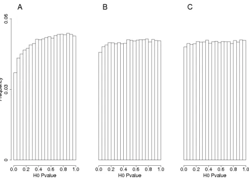
The closed form expression of the non-centrality parameter already revealed that kinship affects power. Comparing the impact of different kinship estimators on power implies to evaluate their ability to guarantee the expected nominal control of false positives under different hypotheses on trait genetic determinism. To this end, we simulated traits influenced by L biallelic QTLs (SNPs).In a first step, QTLs were sampled randomly among the SNPs located on all the chromosomes except one. The chromosome without QTL (further referred to as "H0-chromosome") was used to estimate the false positive rate. All the H0-markers (the markers on the H0-chromosome) were tested with the above mentioned statistical models for each run of simulation. The efficiency of the different estimations of K to control false positives was evaluated by comparing expected and observed quantiles of H0-Pvalues and histograms of H0-Pvalues. In a second step we applied the same procedure, but now sampling the QTLs among the M SNPs (on all chromosomes). A QTL was declared detected when the Pvalue of the corresponding SNP in the genetic model was below the significance threshold. Power of a given model was computed as the number of QTL which were detected. We also applied a less restrictive definition of QTL detection, considering that a QTL could be detected by SNPs located near it. To do so, another analysis was conducted in which markers within a given genetic distance of a QTL were considered H1-markers and the others H0-markers. The realized false discovery rate (FDR) was defined as the proportion of H0-markers among the markers declared significant. Power of QTL detection was estimated by considering that a QTL was detected when at least one of the corresponding H1-markers had a significant Pvalue. This general method will be exemplified with parameters specific to three maize panels described below.
36 Genetic material and genotyping data
The above mentioned power analyses (analytical evaluation of power and simulation based evaluation of alternative methods) were applied to three diversity panels of maize. The first panel
(called C-K) was described in CAMUS-KULANDAIVELU et al. (2006). It is composed of 375 inbred
lines covering American and European diversity. It includes Tropical, Dent and Flint lines. The second and third panels are the Dent and Flint panels of the “Cornfed” project (Dent and
CF-Flint), described in RINCENT et al. (2012). They include lines of the C-K panel and lines derived
from recent breeding schemes. Both are composed of 300 lines. These panels were genotyped with
the 50k SNPs array described in GANAL et al. (2011), as presented in BOUCHET et al. (2013) and
RINCENT et al. (2012). Individuals which had marker missing rate and/or heterozygosity higher than
0.1 and 0.05, respectively, were eliminated. Markers, which had missing rate and/or average heterozygosity higher than 0.2 and 0.15, respectively, were eliminated. In each panel, few individuals were highly related. One individual was removed for pairs identical for more than 98% of the loci. In total 315, 277 and 267 individuals and 44487, 45434, and 44255 markers passed the genotyping filter criteria for the C-K, CF-Dent and CF-Flint designs, respectively. Missing
genotypes (below 2% in both panels) were imputed with the software BEAGLE (BROWNING and
BROWNING 2009). Panels were all adjusted to 267 individuals in order to compare power for a same population size. Individuals removed were chosen at random. To avoid the ascertainment bias noted by GANAL et al. (2011), we only used the markers that were developed by comparing the sequences
of nested association mapping founder lines (PANZEA SNPs, GORE et al. 2009) in the estimation of
admixture and relationship coefficients (29996, 30119 and 29132 markers passed the filter criteria for the C-K, CF-Dent and CF-Flint lines respectively).
Admixture in the CF-Dent and CF-Flint panels was investigated using the SNP data with the
software ADMIXTURE (ALEXANDER et al. 2009), with a number of groups equal to four,
determined according to the cross-validation procedure presented in ADMIXTURE. For the C-K
panel we used the admixture in five groups estimated by CAMUS-KULANDAIVELU et al. (2006) using
55 SSRs chosen for their broad genome coverage and reproducibility. We estimated the
differentiation index among genetic groups (Fst, NEI, 1973) at each marker using the R package
r-hierfstat (GOUDET 2005).
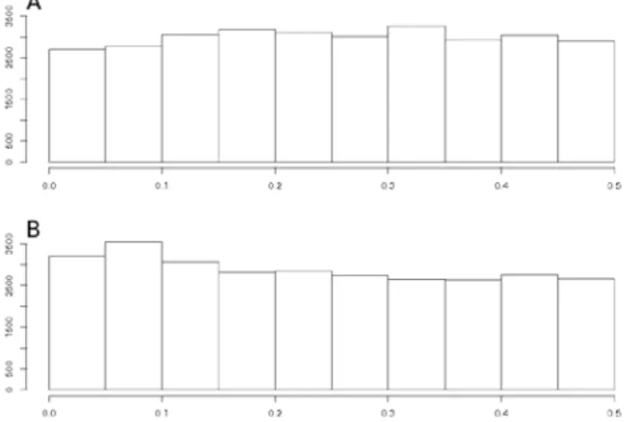
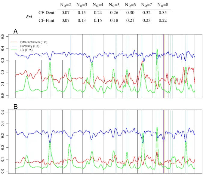
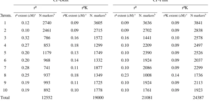
Finally, the relationship between LD and power along the genome can be empirically investigated using two different measures of LD. Raw LD can be estimated as the squared correlation between
37 allelic doses at two loci (r²). Linkage related LD (denoted by r²K) can be estimated using the
algorithm proposed by MANGIN et al. (2012), which corrects r² by K_Freq. LD within these panels
(r²), possibly corrected by K_Freq (r²K), was estimated within a sample of 4000 markers regularly spaced on the physical map.
Specific parameterization
For analytical investigation of power in the three maize panels, the total additive genetic variance
𝜎𝜎𝑔𝑔2 was set to 1000, 𝛽𝛽𝑙𝑙 was set to 17.9, which corresponds to a QTL explaining 8% of the total
genetic variance if it had a minor allele frequency (MAF) of 0.5, 𝜎𝜎𝑒𝑒2 was chosen to get an
heritability of 0.8. Under these hypotheses, analytical power was investigated for an α type I risk
equal to 1,25 10-6
To estimate kinship with the different formulas presented above, we considered that all individuals
were inbred and we estimated 𝜎𝜎𝑙𝑙2as 𝑝𝑝𝑙𝑙(1 − 𝑝𝑝𝑙𝑙).For comparing the different methods for kinship
estimation, we simulated traits influenced by 50 or 100 biallelic QTLs (QTL effects follow a
geometric series as in LANDE and THOMPSON (1990), with parameter a set to 0.96 and 0.98 when 50
or 100 QTLs were simulated, respectively). Sign of allelic effect at a given locus was assigned randomly. Genotypic values of the individuals were calculated as the sum of the allelic effects at these QTLs. Phenotypes were obtained by adding a residual noise following a normal distribution
with mean 0 and variance equal to: 𝜎𝜎𝑔𝑔2�1 ℎ� − 1�, where the heritability ℎ2 2 is set to 0.8.We
performed 100 runs of simulations for each scenario using the R 3.0.0 software (R development Core Team, 2013).Each chromosome was used ten times as the H0-chromosome.For all
simulations, the statistical tests were made with EMMAX (KANG et al. 2010b) to reduce
computational time, and then with ASREML-R (GILMOUR et al. 2006) on the markers which had a
Pvalue below 0.001 with EMMAX. For Pvalues above 0.001, Pvalues obtained with EMMAX and ASREML-R were very close and highly correlated. As investigations of the two criteria for QTL detection (causal factor only or window around it) led to very comparable results with respect to the main focus of our study, results considering a window around causal factor are therefore presented as supplementary information (Table S1).
which led to a risk of 0.05 with a Bonferroni correction on 40 000 tests. We also considered less stringent threshold corresponding to Bonferroni corrections on 4 000 and 400 tests, although the number of tests was always the same. Power under these hypotheses was calculated in R 3.0.0 (R development Core Team, 2013) for each marker.