D. Bell and J. Hong (Eds.): BNCOD 2006, LNCS 4042, pp. 16–35, 2006. © Springer-Verlag Berlin Heidelberg 2006
SD-SQL Server
Witold Litwin1, Soror Sahri1, and Thomas Schwarz2
1CERIA, Paris-Dauphine University
75016 Paris, France
[email protected], [email protected] 2 Santa Clara University,
California, USA [email protected]
Abstract. We present a scalable distributed database system called SD-SQL Server. Its original feature is dynamic and transparent repartitioning of growing tables, avoiding the cumbersome manual repartitioning that characterize current technology. SD-SQL Server re-partitions a table when an insert overflows existing segments. With the comfort of a single node SQL Server user, the SD-SQL Server user has larger tables or gets a faster response time through the dynamic parallelism. We present the architecture of our system, its implementation and the performance analysis. We show that the overhead of our scalable table management should be typically negligible.
1 Introduction
Databases (DBs) are now often huge and grow fast. Large tables are typically hash or range partitioned into segments stored at different storage sites. Current Data Base Management Systems (DBSs) such as SQL Server, Oracle or DB2, provide only static partitioning [1,5,11]. Growing tables have to overflow their storage space after some time. The database administrator (DBA) has then to manually redistribute the database. This operation is cumbersome, users need a more automatic solution, [1].
This situation is similar to that for file users forty years ago in the centralized environment. Efficient management of distributed data presents specific needs. Scalable Distributed Data Structures (SDDSs) address these needs for files, [6,7]. An SDDS scales transparently for an application through distributed splits of its buckets, whether hash, range or k-d based. In [7], we derived the concept of a Scalable Distributed DBS (SD-DBS) for databases. The SD-DBS architecture supports
scalable (distributed relational) tables. As an SDDS, a scalable table accommodates
its growth through the splits of its overflowing segments, located at SD-DBS storage nodes. Also like in an SDDS, we can use hashing, range partitioning, or k-d-trees. The storage nodes can be P2P or grid DBMS nodes. The users or the application, manipulate the scalable tables from a client node that is not a storage node, or from a
peer node that is both, again as in an SDDS. The client accesses a scalable table only
through its specific view, called the (client) image. It is a particular updateable distributed partitioned union view stored at a client. The application manipulates
scalable tables using images directly, or their scalable views. These views involve scalable tables through the references to the images.
Every image, one per client, hides the partitioning of the scalable table and dynamically adjusts to its evolution. The images of the same scalable table may differ among the clients and from the actual partitioning. The image adjustment is lazy. It occurs only when a query to the scalable table finds an outdated image. To prove the feasibility of an SD-DBS, we have built a prototype called SD-SQL Server. The system generalizes the basic SQL Server capabilities to the scalable tables. It runs on a collection of SQL Server linked nodes. For every standard SQL command under SQL Server, there is an SD-SQL Server command for a similar action on scalable tables or views. There are also commands specific to SD-SQL Server client image or node management.
Below we present the architecture and the implementation of our prototype as it stands in its 2005 version. Related papers [14, 15] discuss the user interface. Scalable table processing creates an overhead and our design challenge was to minimize it. The performance analysis proved this overhead negligible for practical purpose. The present capabilities of SQL Server allow a scalable table to reach 250 segments at least. This should suffice for scalable tables reaching very many terabytes. SD-SQL Server is the first system with the discussed capabilities, to the best of our knowledge. Our results pave the way towards the use of the scalable tables as the basic DBMS technology.
Below, Section 2 presents the SD-SQL Server architecture. Section 3 recalls the basics of the user interface. Section 4 discusses our implementation. Section 5 shows experimental performance analysis. Section 6 discusses the related work. Section 7 concludes the presentation.
2 SD-SQL Server Architecture
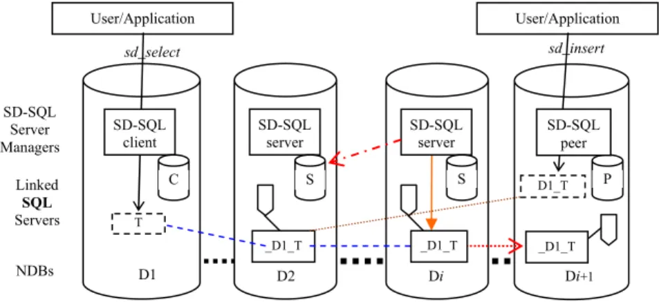
Fig. 1 shows the current SD-SQL Server architecture, adapted from the reference architecture for an SD-DBS in [8]. The system is a collection of SD-SQL Server nodes. An SD-SQL Server node is a linked SQL Server node that in addition is declared as an SD-SQL Server node. This declaration is made as an SD-SQL Server command or is part of a dedicated SQL Server script run on the first node of the collection. We call the first node the primary node. The primary node registers all other current SD-SQL nodes. We can add or remove these dynamically, using specific SD-SQL Server commands. The primary node registers the nodes on itself, in a specific SD-SQL Server database called the meta-database (MDB). An SD-SQL
Server database is an SQL Server database that contains an instance of SD-SQL
Server specific manager component. A node may carry several SD-SQL Server databases.
We call an SD-SQL Server database in short a node database (NDB). NDBs at different nodes may share a (proper) database name. Such nodes form an SD-SQL Server scalable (distributed) database (SDB). The common name is the SDB name. One of NDBs in an SDB is primary. It carries the meta-data registering the current NDBs, their nodes at least. SD-SQL Server provides the commands for scaling up or down an SDB, by adding or dropping NDBs. For an SDB, a node without its NDB is
(an SD-SQL Server) spare (node). A spare for an SDB may already carry an NDB of another SDB. Fig 1 shows an SDB, but does not show spares.
Each manager takes care of the SD-SQL Server specific operations, the user/application command interface especially. The procedures constituting the manager of an NDB are themselves kept in the NDB. They apply internally various SQL Server commands. The SQL Servers at each node entirely handle the inter-node communication and the distributed execution of SQL queries. In this sense, each SD-SQL Server runs at the top of its linked SD-SQL Server, without any specific internal changes of the latter.
An SD-SQL Server NDB is a client, a server, or a peer. The client manages the SD-SQL Server node user/application interface only. This consists of the SD-SQL Server specific commands and from the SQL Server commands. As for the SQL Server, the SD-SQL specific commands address the schema management or let to issue the queries to scalable tables. Such a scalable query may invoke a scalable table through its image name, or indirectly through a scalable view of its image, involving also, perhaps, some static tables, i.e., SQL Server only.
Internally, each client stores the images, the local views and perhaps static tables. These are tables created using the SQL Server CREATE TABLE command (only). It also contains some SD-SQL Server meta-tables constituting the catalog C at Fig 1. The catalog registers the client images, i.e., the images created at the client.
When a scalable query comes in, the client checks whether it actually involves a scalable table. If so, the query must address the local image of the table. It can do it directly through the image name, or through a scalable view. The client searches therefore for the images that the query invokes. For every image, it checks whether it conforms to the actual partitioning of its table, i.e., unions all the existing segments. We recall that a client view may be outdated. The client uses C, as well as some server meta-tables pointed to by C that define the actual partitioning. The manager dynamically adjusts any outdated image. In particular, it changes internally the scheme of the underlying SQL Server partitioned and distributed view, representing the image to the SQL Server. The manager executes the query, when all the images it uses prove up to date.
A server NDB stores the segments of scalable tables. Every segment at a server belongs to a different table. At each server, a segment is internally an SQL Server table with specific properties. First, SD-SQL Server refers to in the specific catalogue in each server NDB, called S in the figure. The meta-data in S identify the scalable table each segment belongs to. They indicate also the segment size. Next, they indicate the servers in the SDB that remain available for the segments created by the splits at the server NDB. Finally, for a primary segment, i.e., the first segment created for a scalable table, the meta-data at its server provide the actual partitioning of the table.
Next, each segment has an AFTER trigger attached, not shown in the figure. It verifies after each insert whether the segment overflows. If so, the server splits the segment, by range partitioning it with respect to the table (partition) key. It moves out enough upper tuples so that the remaining (lower) tuples fit the size of the splitting segment. For the migrating tuples, the server creates remotely one or more new segments that are each half-full (notice the difference to a B-tree split creating a single new segment). Furthermore, every segment in a multi-segment scalable table carries an SQL Server check constraint. Each constraint defines the partition
(primary) key range of the segment. The ranges partition the key space of the table. These conditions let the SQL Server distributed partitioned view to be updateable, by the inserts and deletions in particular. This is a necessary and sufficient condition for a scalable table under SD-SQL Server to be updateable as well.
Finally a peer NDB is both a client and a server NDB. Its node DB carries all the SD-SQL Server meta-tables. It may carry both the client images and the segments. The meta-tables at a peer node form logically the catalog termed P at the figure. This one is operationally, the union of C and S catalogs.
Every SD-SQL Server node is client, server or peer node. The peer accepts every type of NDB. The client nodes only carry client NDBs & server nodes accept server NDBs only. Only a server or peer node can be the primary one or may carry a primary NDB. To illustrate the architecture, Fig 1 shows the NDBs of some SDB, on nodes
D1…Di+1. The NDB at D1 is a client NDB that thus carries only the images and
views, especially the scalable ones. This node could be the primary one, provided it is a peer. It interfaces the applications. The NDBs on all the other nodes until Di are server NDBs. They carry only the segments and do not interface (directly) any applications. The NDB at D2 could be here the primary NDB. Nodes D2…Di could be peers or (only) servers. Finally, the NDB at Di+1 is a peer, providing all the capabilities. Its node has to be a peer node.
The NDBs carry a scalable table termed T. The table has a scalable index I. We suppose that D1 carries the primary image of T, named T at the figure. This image name is also as the SQL Server view name implementing the image in the NDB. SD-SQL Server creates the primary image at the node requesting the creation of a scalable table, while creating the table. Here, the primary segment of table T is supposed at D2. Initially, the primary image included only this segment. It has evolved since, following the expansion of the table at new nodes, and now is the distributed partitioned union-all view of T segments at servers D2…Di. We symbolize this image with the dotted line running from image T till the segment at Di. Peer Di+1 carries a secondary image of table T. Such an image interfaces the application using T on a node other than the table creation one. This image, named
D1_T, for reasons we discuss below, differs from the primary image. It only includes
the primary segment. We symbolize it with the dotted line towards D2 only. Both images are outdated. Indeed, server Di just split its segment and created a new segment of T on Di+1. The arrow at Di and that towards Di+1 represent this split. As the result of the split, server Di updated the meta-data on the actual partitioning of T at server D2 (the dotted arrow from Di to D2). The split has also created the new segment of the scalable index I. None of the two images refers as yet to the new segment. Each will be actualized only once it gets a scalable query to T. At the figure, they are getting such queries, issued using respectively the SD-SQL Server sd_select and sd_insert commands. We discuss the SD-SQL Server command interface in the next sections.
Notice finally that in the figure that the segments of T are all named _D1_T. This represents the couple (creator node, table name). It is the proper name of the segment as an SQL Server table in its NDB. Similarly for the secondary image name, except for the initial ‘_’. The image name is the local SQL Server view name. We explain these naming rules in Section 4.1.
3 Command Interface
3.1 Overview
The application manipulates SD-SQL Server objects essentially through new SD-SQL Server dedicated commands. Some commands address the node management, including the management of SDBs, NDBs. Other commands manipulate the scalable tables. These commands perform the usual SQL schema manipulations and queries that can however now involve scalable tables (through the images) or (scalable) views of the scalable tables. We call the SD-SQL Server commands scalable. A scalable command may include additional parameters specific to the scalable environment, with respect to its static (SQL Server) counterpart. Most of scalable commands apply also to static tables and views. The application using SD-SQL Server may alternatively directly invoke a static command. Such calls are transparent to SD-SQL Server managers. Spl User/Application User/Application Linked SQL Servers D1 NDBs D2 Di Di+1 _D1_T SD-SQL server SD-SQL server SD-SQL client S S P C D1_T SD-SQL Server Managers _D1_T _D1_T T sd_select SD-SQL peer sd_insert
Fig. 1. SD-SQL Server Architecture
Details of all the SD-SQL Server commands are in [14, 15]. The rule for an SD-SQL Server command performing an SQL operation is to use the SQL command name (verb) prefixed with ‘sd_’ and with all the blanks replaced with ‘_’. Thus, e.g., SQL SELECT became SD-SQL sd_select, while SQL CREATE TABLE became sd_create_table. The standard SQL clauses, with perhaps additional parameters follow the verb, specified as usual for SQL. The whole specification is however within additional quotes ‘ ’. The rationale is that SD-SQL Server commands are implemented as SQL Server stored procedures. The clauses pass to SQL Server as the parameters of a stored procedure and the quotes around the parameter list are mandatory.
The operational capabilities of SD-SQL Server should suffice for many applications. The SELECT statement in a scalable query supports the SQL Server allowed selections, restrictions, joins, sub-queries, aggregations, aliases…etc. It also allows for the INTO clause that can create a scalable table. However, the queries to the scalable multi-database views are not possible at present. The reasons are the limitation of the SQL Server meta-tables that SD-SQL Server uses for the parsing.
Moreover, the sd_insert command over a scalable table lets for any insert accepted by SQL Server for a distributed partitioned view. This can be a new tuple insert, as well as a multi-tuple insert through a SELECT expression, including the INTO clause. The
sd_update and sd_delete commands offer similar capabilities. In contrast, some of
SQL Server specific SQL clauses are not supported at present by the scalable commands; for instance, the CASE OF clause.
We recall the SD-SQL Server command interface by the motivating example. modelled upon our benchmark application that is SkyServer DB, [2].
3.2 Motivating Example
A script file creates the first ever (primary) SD-SQL Server (scalable) node at a collection of linked SQL Server nodes. We can create the primary node as a peer or a server, but not as a client. After that, we can create additional nodes using the
sd_create_node command. Here, the script has created the primary SD-SQL Server
node at SQL Server linked node at our Dell1 machine. We could set up this node as server or peer, we made the latter choice. The following commands issued at Dell1 create then further nodes, alter Dell3 type to peer, and finally create our SkyServer SDB at Dell1:
sd_create_node ‘Dell2’ /* Server by default */; sd_create_node ‘Dell3, ‘client’ ;
sd_create_node ‘Ceria1’,’peer’
sd_alter_ node ‘Dell3’, ‘ADD server’ ; sd_create_scalable_database ‘SkyServer, ‘Dell1’
Our SDB has now one NDB termed SkyServer. This NDB is the primary one of the SDB and is a server NDB. To query , SkyServer one needs at least one client or peer NDB. We therefore append a client NDB at Dell3 client node:
sd_create_node_database ‘SkyServer’, ‘Dell3’, ‘client’
From now on, Dell3 user opens Skyserver SDB through the usual SQL Server USE
Skyserver command (which actually opens Dell3.Skyserver NDB). The Skyserver
users are now furthermore able to create scalable tables. The Dell3 user starts with a
PhotoObj table modelled on the static table with the same name, [2]. The user wishes
the segment capacity of 10000 tuples. S/he chooses this parameter for the efficient distributed query processing. S/he also wishes the objid key attribute to be the partition key. In SD-SQL Server, a partition key of a scalable table has to be a single key attribute. The requirement comes from SQL Server, where it has to be the case of a table, or tables, behind a distributed partitioned updatable view. The key attribute of
PhotoObj is its objid attribute. The user issues the command:
sd_create_table ‘PhotoObj (objid BIGINT PRIMARY KEY…)’, 10000
We did not provide the complete syntax, using ‘…’ to denote the rest of the scheme beyond the key attribute. The objid attribute is the partition key implicitly, since it is here the only key attribute. The user creates furthermore a scalable table Neighbors, modelled upon the similar one in the static Skyserver. That table has three key
attributes. The objid is one of them and is the foreign key of PhotoObj. For this reason, the user wishes it to be the partition key. The segment capacity should now be 500 tuples. Accordingly, the user issues the command:
sd_create_table ‘Neighbors (htmid BIGINT, objid BIGINT, Neighborobjid BIGINT) ON PRIMARY KEY…)’, 500, ‘objid’
The user indicated the partition key. The implicit choice would go indeed to htmid, as the first one in the list of key attributes. The Dell3 user decides furthermore to add attribute t to PhotoObj and prefer a smaller segment size:
sd_alter_table ‘PhotoObj ADD t INT, 1000
Next the user decides to create a scalable index on run attribute:
sd_create_index ‘run_index ON Photoobj (run)'
Splits of PhotoObj will propagate run_index to any new segment.
The PhotoObj creation command created the primary image at Dell3. The Dell3 user creates now the secondary image of PhotoObj at Ceria1 node for the SkyServer user there::
sd_create_image ‘Ceria1’, ‘PhotoObj’
The image internal name is SD.Dell3_Photoobj, as we discuss in Section 0 and [15]. The Ceria1 user who wishes a different local name such as PhotoObj uses the SQL Server CREATE VIEW command. Once the Ceria1 user does not need its image anymore, s/he may remove it through the command:
sd_drop_image 'SD.Dell3_Photoobj'
Assuming that the image was not dropped however yet, our Dell3 user may open
Skyserver SDB and query PhotoObj:
USE Skyserver /* SQL Server command */
sd_insert ‘INTO PhotoObj SELECT * FROM Ceria5.Skyserver-S.PhotoObj sd_select ‘* FROM PhotoObj’ ;
sd_select ‘TOP 5000 * INTO PhotoObj1 FROM PhotoObj’, 500
The first query loads into our PhotoObj scalable table tuples from some other
PhotoObj table or view created in some Skyserver DB at node Ceria5. This DB could
be a static, i.e., SQL Server only, DB. It could alternatively be an NDB of “our”
Skyserver DB. The second query creates scalable table PhotoObj1 with segment size
of 500 and copies there 5000 tuples from PhotoObj, having the smallest values of
objid. See [15] for examples of other scalable commands.
4 Command Processing
We now present the basics of SD_SQL Server command processing. We start with the naming rules and the meta-tables. Next, we discuss the scalable table evolution.
We follow up with the image processing. For more on the command processing see [14].
4.1 Naming Rules
SD-SQL Server has its own system objects for the scalable table management. These are the node DBs, the meta-tables, the stored procedures, the table and index segments and the images. All the system objects are implemented as SQL Server objects. To avoid the name conflicts, especially between the SQL Server names created by an SD-SQL Server application, there are the following naming rules, partly illustrated at Fig. 1. Each NDB has a dedicated user account ‘SD’ for SD-SQL Server itself. The application name of a table, of a database, of a view or of a stored procedure, created at an SD-SQL Server node as public (dbo) objects, should not be the name of an SD-SQL Server command. These are SD-SQL server keywords, reserved for its commands (in addition to the same rule already enforced by SQL Server for its own SQL commands). The technical rationale is that SD-SQL Server commands are public stored procedures under the same names. An SQL Server may call them from any user account.
A scalable table T at a NDB is a public object, i.e., its SQL Server name is dbo.T. It is thus unique regardless of the user that has created it1. In other words, two different SQL Server users of a NDB cannot create each a scalable table with the proper name T. They can still do it for the static tables of course. Besides, two SD-SQL Server users at different nodes may each create a scalable table with the proper name T.
A segment of scalable table created with proper name T, at SQL Server node N, bears for any SQL Server the table name SD._N_T within its SD-SQL Server node (its NDB more specifically, we recall). We recall that SD-SQL Server locates every segment of a scalable table at a different node.
A primary image of a scalable table T bears the proper name T. Its global name within the node is dbo.T. This is also the proper name of the SQL Server distributed partitioned view implementing the primary view.
Any secondary image of scalable table created by the application with proper name
T, within the table names at client or peer node N, bears the global name at its node SD.N_T. In Fig 1, e.g., the proper name of secondary image denoted T (2) would
actually be D1_T.
We recall that since SD-SQL Server commands are public stored procedures, SQL Server automatically prefixes all the proper names of SD-SQL public objects with dbo. in every NDB, to prevent a name conflict with any other owner within NDB. The rules avoid name conflicts between the SD-SQL Server private application objects and SD-SQL system objects, as well as between SD-SQL Server system objects themselves. See [14] for more examples of the naming rules.
4.2 Meta-tables
These tables constitute internally SQL Server tables searched and updated using the stored procedures with SQL queries detailed in [8]. All the meta-tables are under the user name SD, i.e., are prefixed within their NDB with ‘SD.’.
The S-catalog exists at each server and contains the following tables.
- SD.RP (SgmNd, CreatNd, Table). This table at node N defines the scalable
distributed partitioning of every table Table originating within its NDB, let it be D, at some server CreatNd, and having its primary segment located at N. Tuple (SgmNd, CreatNd, Table) enters N.D.SD.RP each time Table gets a new segment at some node SgmNd. For example, tuple (Dell5, Dell1, PhotoObj) in Dell2.D.SD.RP means that scalable table PhotoObj was created in Dell1.D, had its primary segment at Dell2.D, and later got a new segment _Dell1_PhotoObj in Dell5.D. We recall that a segment proper name starts with ‘_’, being formed as in Fig. 1.
- SD.Size (CreatNd, Table, Size). This table fixes for each segment in some NDB at
SQL Server node N the maximal size (in tuples) allowed for the segment. For instance, tuple (Dell1, PhotoObj, 1000) in Dell5.DB1.SD.Size means that the maximal size of the Dell5 segment of PhotoObj scalable table initially created in
Dell1.DB1 is 1000. We recall that at present all the segment of a scalable table
have the same sizes.
- SD.Primary (PrimNd, CreatNd, Table). A tuple means here that the primary
segment of table T created at client or peer CreatNd is at node PrimNd. The tuple points consequently to SD.RP with the actual partitioning of T. A tuple enters
N.SD.Primary when a node performs a table creation or split and the new segment
lands at N. For example, tuple (Dell2, Dell1, PhotoObj) in SD.Primary at node
Dell5 means that there is a segment _Dell1_PhotoObj resulting from the split of PhotoObj table, created at Dell1 and with the primary segment at Dell2.
The C-catalog has two tables:
- Table SD.Image (Name, Type, PrimNd,Size) registers all the local images. Tuple (I, T, P, S) means that, at the node, there is some image with the (proper) name I, primary if T = .true, of a table using P as the primary node that the client sees as having S segments. For example, tuple (PhotoObj, true, Dell2, 2) in
Dell1.SD.C-Image means that there is a primary image dbo.PhotoObj at Dell1 whose table
seems to contain two segments. SD-SQL Server explores this table during the scalable query processing.
- Table SD.Server (Node) provides the server (peer) node(s) at the client disposal for the location of the primary segment of a table to create. The table contains basically only one tuple. It may contain more, e.g., for the fault tolerance or load balancing.
Finally, the P-catalogue, at a peer, is simply the union of C-catalog and S-catalog. In addition, each NDB has two tables:
- SD.SDBNode (Node). This table points towards the primary NDB of the SDB. It could indicate more nodes, replicating the SDB metadata for fault-tolerance or load balancing.
- SD.MDBNode (Node). This table points towards the primary node. It could indicate
There are also meta-tables for the SD-SQL Server node management and SDB management. These are the tables:
- SD.Nodes (Node, Type). This table is in the MDB. Each tuple registers an SD-SQL
Server node currently forming the SQL configuration. We recall that every SD-SQL Server node is an SD-SQL Server linked server declared SD-SD-SQL Server node by the initial script or the sd_create_node command. The values of Type are ‘peer’, ‘server’ or ‘client’.
- SD.SDB (SDB_Name, Node, NDBType). This table is also in the MDB. Each tuple
registers an SDB. For instance, tuple (DB1, Dell5, Peer) means that there is an SDB named DB1, with the primary NDB at Dell5, created by the command
sd_create_scalable_database ‘DB1’, ‘Dell5’, ‘peer’.
- SD.NDB (Node, NDBType). This meta-table is at each primary NDB. It registers all
the NDBs currently composing the SDB. The NDBType indicates whether the NDB is a peer, server or client.
4.3 Scalable Table Evolution
A scalable table T grows by getting new segments, and shrinks by dropping some. The dynamic splitting of overflowing segments performs the former. The merge of under-loaded segments may perform the latter. There seems to be little practical interest for merges, just as implementations of B-tree merges are rare. We did not consider them for the current prototype. We only present the splitting now. The operation aims at several goals. We first enumerate them, then we discuss the processing:
1. The split aims at removing the overflow from the splitting segment by migrating some of its tuples into one or several new segment(s). The segment should possibly stay at least half full. The new segments should end up half full. The overall result is then at least the typical “good” load factor of 69 %.
2. Splitting should not delay the commit of the insert triggering it. The insert could timeout otherwise. Through the performance measures in Section 0, we expect the split to be often much longer than a insert.
3. The allocation of nodes to the new segments aims at the random node load balancing among the clients and /or peers. However, the splitting algorithm also allocates the same nodes to the successive segments of different scalable tables of the same client. The policy aims at faster query execution, as the queries tend to address the tables of the same client.
4. The concurrent execution of the split and of the scalable queries should be serializable. A concurrent scalable query to the tuples in an overflowing segment, should either access them before any migrate, or only when the split is over.
We now show how SD-SQL Server achieves these goals. The creation of a new segment for a scalable table T occurs when an insert overflows the capacity of one of its segments, declared in local SD.Size for T. At present, all the segments of a scalable table have the same capacity, denoted b below, and defined in the sd_create_table command. The overflow may consist of arbitrarily many tuples, brought by a single
sd_insert command with the SELECT expression (unlike in a record-at-the-time
segments. More precisely, we may distinguish the cases of a (single segment) tuple
insert split, of a single segment bulk insert split and of a multi-segment (insert) split.
The bulk inserts correspond to the sd_insert with the SELECT expression.
In every sd_insert case, the AFTER trigger at every segment getting tuples tests for overflow, [8]. The positive result leads to the split of the segment, according to the following segment partitioning scheme. We first discuss the basic case of the partition key attribute being the (single-attribute) primary key. We show next the case of the multi-attribute key, where the partition key may thus present duplicates. We recall that the partition key under SQL Server must be a (single) key attribute. In every case, the scheme adds N ≥ 1 segments to the table, with N as follows.
Let P be the (overflowing) set of all the tuples in one of, or the only, overflowing segment of T, ordered in ascending order by the partition key. Each server aims at cutting its P, starting from the high-end, into successive portions P1…PN consisting
each of INT (b/2) tuples. Each portion goes to a different server to become a possibly half-full new segment of T. The number N is the minimal one leaving at most b tuples in the splitting segment. To fulfil goal (1) above, we thus always have N = 1 for a tuple insert, and the usual even partitioning (for the partition key without duplicates). A single segment bulk insert basically leads to N ≥ 1 half-full new segments. The splitting one ends up between half-full and full. We have in both cases:
N = ⎡(Card(P) – b) / INT (b/2)⎤
The same scheme applies to every splitting segment for a multiple bucket insert. If the partition key presents the duplicates, the result of the calculus may differ a little in practice, but arbitrarily in theory. The calculus of each Pi incorporates into it all the
duplicates of the lowest key value, if there is any. The new segment may start more than half-full accordingly, even overflowing in an unlikely bad case. The presence of duplicates may in this way decrease N. It may theoretically even happen that all the partition key values amount to a single duplicate. We test this situation in which case no migration occurs. The split waits till different key values come in. The whole duplicate management is potentially subject of future work optimizing the Pi calculus.
The AFTER trigger only tests for overflow, to respond to goal (2). If necessary, it launches the actual splitting process as an asynchronous job called splitter (for performance reasons, see above). The splitter gets the segment name as the input parameter. To create the new segment(s) with their respective portions, the splitter acts as follows. It starts as a distributed transaction at the repeatable read isolation level. SQL Server uses then the shared and exclusive tuple locks according to the basic 2PL protocol. The splitter first searches for PrimNd of the segment to split in
Primary meta-table. If it finds the searched tuple, SQL Server puts it under a shared
lock. The splitter requests then an exclusive lock on the tuple registering the splitting segment in RP of the splitting table that is in the NDB at PrimNd node. As we show later, it gets the lock if there are no (more) scalable queries or other commands in progress involving the segment. Otherwise it would encounter at least a shared lock at the tuple. SQL Server would then block the split until the end of the concurrent operation. In unlikely cases, a deadlock may result. The overall interaction suffices to provide the serializability of every command and of a split, [14]. If the splitter does not find the tuple in Primary, it terminates. As it will appear, it means that a delete of the table occurred in the meantime.
From now on, there cannot be a query in progress on the splitting segment; neither can another splitter lock it. It should first lock the tuple in RP. The splitter safely verifies the segment size. An insert or deletion could change it in the meantime. If the segment does not overflow anymore, the splitter terminates. Next, it determines N as above. It finds b in the local SD.Size meta-table. Next, it attempts to find N NDBs without any segment of T as yet. It searches for such nodes through the query to NDB meta-table, requesting every NDB in the SDB which is a server or peer and not yet in
RP for T. Let M ≥ 0 be the number of NDBs found. If M = N, then the splitter
allocates each new segment to a node. If M > N, then it randomly selects the nodes for the new segments. To satisfy goal (3) above, the selection is nevertheless driven, at the base of the randomness generation, by T creation NDB name. Any two tables created by the same client node share the same primary NDB, have their 1st
secondary segments at the same (another) server as well etc… One may expect this policy to be usually beneficial for the query processing speed. At the expense however, perhaps of the uniformity of the processing and storage load among the server NDBs.
If M < N, it means that the SDB has not enough of NDBs to carry out the split. The splitter attempts then to extend the SDB with new server or peer NDBs. It selects (exclusively) possibly enough nodes in the meta-database which are not yet in the SDB. It uses the meta-tables Nodes and SDB in the MDB and NDB at the primary SDB node. If it does not succeeds the splitting halts with a message to the administrator. This one may choose to add nodes using sd_create_node command. Otherwise, the splitter updates the NDB meta-table, asks SQL Server to create the new NDBs (by issuing the sd_create_node_database command) and allocates these to the remaining new segment(s).
Once done with the allocation phase, the splitter creates the new segments. Each new segment should have the schema of the splitting one, including the proper name, the key and the indexes, except for the values of the check constraint as we discuss below. Let Sbe here the splitting segment, let p be p = INT (b/2), let c be the key, and let Si denote the new segment at node Ni, destined for portion Pi. The creation of the
new segments loops for i = 1…N as follows.
It starts with the SQL Server query in the form of :
SELECT TOP p (*) WITH TIES INTO Ni.Si FROM S ORDER BY c ASC The option “with ties” takes care of the duplicates2. Next, the splitter finds the partition key c of S using the SQL Server system tables and alters Si scheme
accordingly. To find c, it joins SQL Server system tables information_schema.Tables
and information_schema.TABLE_CONSTRAINTS on the TABLE_SCHEMA,
CONSTRAINT_SCHEMA and CONSTRAINT_NAME columns. It also determines the
indexes on S using the SQL Server stored procedure sp_helpindex. It creates then the same indexes on Si using the SQL Server create index statements. Finally, it creates
the check constraint on Si as we describe soon. Once all this done, it registers the new
2 Actually, it first performs the test whether the split can occur at all, as we discussed, using the
segment in the SD-SQL Server meta-tables. It inserts the tuples describing Si into (i) Primary table at the new node, and (ii) RP table at the primary node of T. It also
inserts the one with the Si size into Size at the new node. As the last step, it deletes from Sthe copied tuples. It then moves to the processing of next Pi if any remains.
Once the loop finishes, the splitter commits which makes SQL Server to release all the locks.
The splitter computes each check constraint as follows. We recall that, if defined for segment S, this constraint C(S) defines the low l and/or the high h bounds on any partition key value c that segment may contain. SQL Server needs for updates through a distributed partitioned view, a necessity for SD-SQL Server. Because of our duplicates management, we have: C(S) = { c : l ≤ c < h }. Let thus hi be the highest
key values in portion Pi> 1, perhaps, undefined for P1.Let also hN + 1 be the highest key
remaining in the splitting segment. Then the low and high bounds for new segment Si
getting Pi is l = hi+1 and h = hi .The splitting segment keeps its l, if it had any, while it
gets as new h the value h’ = hN+1, where h’ < h. The result makes T always range
partitioned.
4.4 Image Processing
4.4.1 Checking and Adjustment
A scalable query invokes an image of some scalable table, let it be T. The image can be primary or secondary, invoked directly or through a (scalable) view. SD-SQL Server produces from the scalable query, let it be Q, an SQL Server query Q’ that it passes for the actual execution. Q’ actually addresses the distributed partitioned view defining the image that is dbo.T. It should not use an outdated view. Q’ would not process the missing segments and Q could return an incorrect result.
Before passing Q’ to SQL Server, the client manager first checks the image correctness with respect to the actual partitioning of T. RP table at T primary server let to determine the latter. The manager retrieves from Image the presumed size of T, in the number of segments, let it be SI. It is the Size of the (only) tuple in Image with Name = ‘T’. The client also retrieves the PrimNd of the tuple. It is the node of the
primary NDB of T, unless the command sd_drop_node_database or sd_drop_node had for the effect to displace it elsewhere. In the last case, the client retrieves the
PrimNd in the SD.SDB meta-table. We recall that this NDB always has locally the
same name as the client NDB. They both share the SDB name, let it be D. Next, the manager issues the multi-database SQL Server query that counts the number of segments of T in PrimNd.D.SD.RP. Assuming that SQL Server finds the NDB, let SA
be this count. If SA = 0, then the table was deleted in the meantime. The client
terminates the query. Otherwise, it checks whether SI = SA. If so, the image is correct.
Otherwise, the client adjusts the Size value to SA. It also requests the node names of T
segments in PrimNd.D.SD.RP. Using these names, it forms the segment names as already discussed. Finally, the client replaces the existing dbo.T with the one involving all newly found segments.
The view dbo.T should remain the correct image until the scalable query finishes exploring T. This implies that no split modifies partitioning of T since the client requested the segment node names in PrimNd.D.SD.RP, until Q finishes
mani-pulating T. Giving our splitting scheme, this means in practice that no split starts in the meantime the deletion phase on any T segment. To ensure this, the manager requests from SQL Server to process every Q as a distributed transaction at the repeatable read isolation level. We recall that the splitter uses the same level. The counting in PrimNd.D.SD.RP during Q processing generates then a shared lock at each selected tuple. Any split of T in progress has to request an exclusive lock on some such tuple, registering the splitting segment. According to its 2PL protocol, SQL Server would then block any T split until Q terminates. Vice versa, Q in progress would not finish, or perhaps even start the SA count and the T segment names retrieval
until any split in progress ends. Q will take then the newly added T segments into account as well. In both cases, the query and split executions remain serializable.
Finally, we use a lazy schema validation option for our linked SQL Servers, [1, 10]. When starting Q’, SQL Server drops then the preventive checking of the schema of any remote table referred to in a partitioned view. The run-time performance obviously must improve, especially for a view referring to many tables [9]. The potential drawback is a run-time error generated by a discrepancy between the compiled query based on the view, dbo.T in our case, and some alterations of schema
T by SD-SQL Server user since, requiring Q recompilation on the fly.
Example. Consider query Q to SkyServer peer NDB at the Ceria1:
sd_select ‘* from PhotoObj’
Suppose that PhotoObj is here a scalable table created locally, and with the local primary segment, as typically for a scalable table created at a peer. Hence, Q’ should address dbo.PhotoObj view and is here:
SELECT * FROM dbo.PhotoObj
Consider that Ceria1 manager processing Q finds Size = 1 in the tuple with of
Name = ‘PhotoObj’ retrieved from its Image table. The client finds also Ceria1 in the PrimeNd of the tuple. Suppose further that PhotoObj has in fact also two secondary
segments at Dell1 and Dell2. The counting of the tuples with Table = ‘PhotoObj’ and
CreatNd = ’Ceria1’ in Ceria1.SkyServer.SD.RP reports then SA = 3. Once SQL Server
retrieves the count, it would put on hold any attempt to change T partitioning till Q ends. The image of PhotoObj in dbo.PhotoObj turns out thus not correct. The manager should update it. It thus retrieves from Ceria1.SkyServer.SD.RP the SgmNd values in the previously counted tuples. It gets {Dell1, Dell2, Ceria1}. It generates the actual segment names as ‘_Dell1_PhotoObj’ etc. It recreates dbo.PhotoObj view and updates Size to 3 in the manipulated tuple in its Image table. It may now safely pass Q’ to SQL Server.
4.4.2 Binding
A scalable query consists of a query command to an SD-SQL Server client (peer) followed by a (scalable) query expression. We recall that these commands are
sd_select, sd_insert, sd_update and sd_delete. Every scalable query, unlike a static
one, starts with an image binding phase that determines every image on which a table or a view name in a query depends. The client verifies every image before it passes to SQL Server any query to the scalable table behind the image. We now present the
processing of scalable queries under SD-SQL Server. We only discuss image binding and refer to more documentation for each command to [14].
The client (manager) parses every FROM clause in the query expression, including every sub-query, for the table or view names it contains. The table name can be that of a scalable one, but then is that of its primary image. It may also be that of a secondary image. Finally, it can be that of a static (base) table. A view name may be that of a scalable view or of a static view. Every reference has to be resolved. Every image found has to be verified and perhaps adjusted before SD-SQL Server lets SQL Server to use it, as already discussed.
The client searches the table and view names in FROM clauses, using the SQL Server xp_sscanf function, and some related processing. This function reads data from the string into the argument locations given by each format argument. We use it to return all the objects in the FROM clause. The list of objects is returned as it appears in the clause FROM, i.e. with the ‘,’ character. Next, SD-SQL Server parses the list of the objects and takes every object name alone by separating it from it FROM clause list. For every name found, let it be X, assumed a proper name, the client manager proceeds as follows:
It searches for X within Name attribute of its Image table. If it finds the tuple with
X, then it puts X aside into check_image list, unless it is already there.
Otherwise, the manager explores with T the sysobjects and sysdepends tables of SQL Server. Table sysobjects provides for each object name its type (V = view, T = base table…) and internal Id, among other data. Table sysdepends provides for each view, given its Id, its local (direct) dependants. These can be tables or views themselves. A multi-database base view does not have direct remote dependants in
sysobjects. That is why we at present do not allow scalable multi-database views. The
client searches, recursively if necessary, for any dependants of X that is a view that has a table as dependant in sysobjects or has no dependant listed there. The former may be an image with a local segment. The latter may be an image with remote segments only. It then searches Image again for X. If it finds it, then it attempts to add it to check_image.
Once all the images have been determined, i.e., there is no FROM clause in the query remaining for the analysis, the client verifies each of them, as usual. The verification follows the order on the image names. The rationale is to avoid the (rare) deadlock, when two outdated images could be concurrently processed in opposite order by two queries to the same manager. The adjustment generates indeed an exclusive lock on the tuple in Image. After the end of the image binding phase, the client continues with the specific processing of each command that we present later.
With respect to the concurrent command processing, the image binding phase results for SQL Server in a repeatable read level distributed transaction with shared locks or exclusive locks on the tuples of the bound images in Image tables and with the shared locks on all the related tuples in various RP tables. The image binding for one query may thus block another binding the same image that happened to be outdated. A shared lock on RP tuple may block a concurrent split as already discussed. We’ll show progressively that all this behaviour contributed to the serializability of the whole scalable command processing under SD-SQL Server.
5 Performance Analysis
To validate the SD-SQL Server architecture, we evaluated its scalability and efficiency over some Skyserver DB data [2]. Our hardware consisted of 1.8 GHz P4 PCs with either 785 MB or 1 GB of RAM, linked by a 1 Gbs Ethernet. We used the SQL Profiler to take measurements. We measured split times and query response times under various conditions. The split time was from about 2.5 s for a 2-split of 1000-tuple PhotoObj segment, up to 150 seconds for a 5-split of a 160 000 tuple segment. Presence of indexes naturally increased this time, up to almost 200 s for the 5-split of a 160 000 tuple segment with three indexes.
The query measures included the overhead of the image checking alone, of image adjustment and of image binding for various queries, [14]. Here, we discuss two queries:
(Q1) sd_select ‘COUNT (*) FROM PhotoObj’
(Q2) sd_select 'top 10000 x.objid from photoobj x, photoobj y where x.obj=y.obj
and x.objid>y.objid
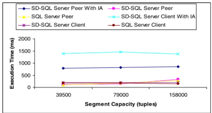
Query (Q1) represents the rather fast queries, query (Q2) the complex ones, because of its double join and larger result set. The measures of (Q1) concern the execution time under various conditions, Fig. 2. The table had two segments of various sizes. We measured (Q1) at SD-SQL Server peer, where the Image and RP tables are at the same node, and at a client where they are at different nodes. We executed (Q1) with image checking (IC) only, and with the image adjustment (IA). We finally compared these times to those of executing (Q1) as an SQL Server, i.e., without even IC. As the curves show, IC overhead appeared always negligible. (Q1) always executed then under 300 msec. In contrast the IA overhead is relatively costly. On a peer node it is about 0.5s, leading to the response time of 0.8sec. On a client node, it increases to about 1s, leading to (Q1) response time of 1.5s. The difference is obviously due to the remote accesses to RP table. Notice that IA time is constant, as one could expect. We used the LSV option, but the results were about the same without it.
The measures of (Q2) representing basically longer to process typical queries than (Q1), involved PhotoObj with almost 160 K tuples spreading over two, three or four segments. The query execution time with IC only (or even without, directly by SQL Server) is now between 10 – 12 s. The IA overhead is about or little over 1 s. It grows a little since SQL Server ALTER VIEW operation has more remote segments to access for the check constraint update (even if it remains in fact the same, which indicates a clear path for some optimizing of this operation under SQL Server). IA overhead becomes relatively negligible, about 10 % of the query cost. We recall that IA should be in any case a rare operation.
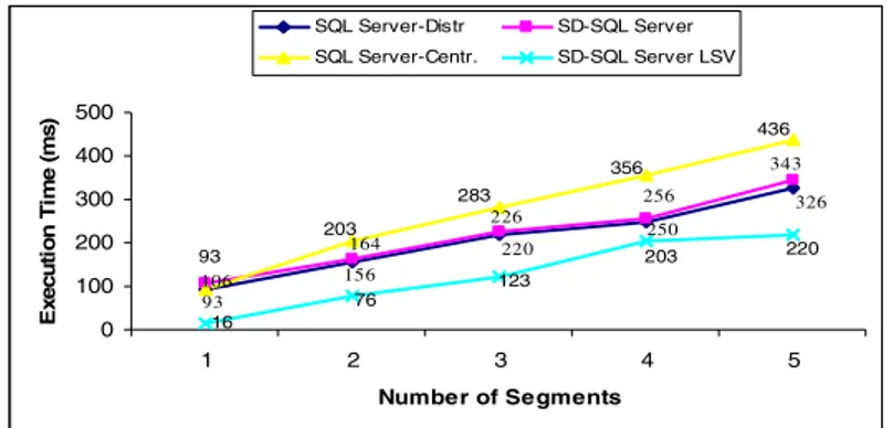
Finally, we have measured again (Q1) on our PhotoObj scalable table as it grows under inserts. It had successively 2, 3, 4 and 5 segments, generated each by a 2-split. The query counted at every segment. The segment capacity was 30K tuples. We aimed at the comparison of the response time for an SD-SQL Server user and for the one of SQL Server. We supposed that the latter (i) does not enters the manual repartitioning hassle, or, alternatively, (ii) enters it by 2-splitting manually any time the table gets new 30K tuples, i.e., at the same time when SD-SQL Server would trigger its split. Case (i) corresponds to the same comfort as that of an SD-SQL Server
0 500 1000 1500 2000 39500 79000 158000
Segment Capacity (tuples)
E x ecuti on Ti m e (m s)
SD-SQL Server Peer With IA SD-SQL Server Peer SQL Server Peer SD-SQL Server Client With IA SD-SQL Server Client SQL Server Client
Fig. 2. Query (Q1) execution performance
9862.4 11578.66 10898 13036.5 14071.66 11712 0 2000 4000 6000 8000 10000 12000 14000 16000 2 3 4 Number of Segments E x e c ut ion Ti me ( m s ) IA IC
Fig. 3. Query (Q2) with image checking only (IC) and with image adjustment (IA)
user. The obvious price to pay for an SQL Server user is the scalability, i.e., the worst deterioration of the response time for a growing table. In both cases (i) and (ii) we studied the SQL Server query corresponding to (Q1) for a static table. For SD-SQL Server, we measured (Q1) with and without the LSV option.
The figure displays the result. The curve named “SQL Server Centr.” shows the case (i), i.e., of the centralized PhotoObj. The curve “SQL Server Distr.” reflects the manual reorganizing (ii). The curve shows the minimum that SD-SQL Server could reach, i.e., if it had zero overhead. The two other curves correspond to SD-SQL Server.
We can see that SD-SQL Server processing time is always quite close to that of (ii) by SQL Server. Our query-processing overhead appears only about 5%. We can also see that for the same comfort of use, i.e., with respect to case (i), SD-SQL Server without LZV speeds up the execution by almost 30 %, e.g., about 100 msec for the largest table measured. With LZV the time decreases there to 220 msec. It improves thus by almost 50 %. This factor characterizes most of the other sizes as well. All these results prove the immediate utility of our system.
93 156 220 250 326 106 164 226 256 343 283 203 93 356 436 220 203 123 76 16 0 100 200 300 400 500 1 2 3 4 5 Number of Segments E x e c u ti o n Ti m e ( m s ) SQL Server-Distr SD-SQL Server SQL Server-Centr. SD-SQL Server LSV
Fig. 4. Query (Q1) execution on SQL Server and SD-SQL Server (Client/Peer) Notice further that in theory SD-SQL Server execution time could remain constant and close to that of a query to a single segment of about 30 K tuples. This is 93 ms in our case. The timing observed practice grows in contrast, already for the SQL Server. The result seems to indicate that the parallel processing of the aggregate functions by SQL Server has still room for improvement. This would further increase the superiority of SD-SQL Server for the same user’s comfort.
6 Related Works
Parallel and distributed database partitioning has been studied for many years, [13]. It naturally triggered the work on the reorganizing of the partitioning, with notable results as early as in 1996, [12]. The common goal was global reorganization, unlike for our system.
The editors of [12] contributed themselves with two on-line reorganization methods, called respectively new-space and in-place reorganization. The former method created a new disk structure, and switches the processing to it. The latter approach balanced the data among existing disk pages as long as there was room for the data. Among the other contributors to [12], one concerned a command named ‘Move Partition Boundary’ for Tandem Non Stop SQL/MP. The command aimed on on-line changes to the adjacent database partitions. The new boundary should decrease the load of any nearly full partition, by assigning some tuples into a less loaded one. The command was intended as a manual operation. We could not ascertain whether it was ever implemented.
A more recent proposal of efficient global reorganizing strategy is in [11]. One proposes there an automatic advisor, balancing the overall database load through the periodic reorganizing. The advisor is intended as a DB2 offline utility. Another attempt, in [4], the most recent one to our knowledge, describes yet another sophisticated reorganizing technique, based on database clustering. Called AutoClust, the technique mines for closed sets, then groups the records according to the resulting attribute clusters. AutoClust processing should start when the average query response time drops below a user defined threshold. We do not know whether AutoClust was put into practice.
With respect to the partitioning algorithms used in other major DBMSs, parallel DB2 uses (static) hash partitioning. Oracle offers both hash and range partitioning, but over the shared disk multiprocessor architecture only. Only SQL Server offers the updatable distributed partitioned views. This was the major rationale for our choice, since scalable tables have to be updatable. How the scalable tables may be created at other systems remains thus an open research problem.
7 Conclusion
The proposed syntax and semantics of SD-SQL Server commands make the use of scalable tables about as simple as that of the static ones. It lets the user/application to easily take advantage of the new capabilities of our system. Through the scalable distributed partitioning, they should allow for much larger tables or for a faster response time of complex queries, or for both.
The current design of our interface is geared towards a “proof of concept” prototype. It is naturally simpler than a full-scale system. Further work should expand it. Among the challenges at the processing level, notice that there is no user account management for the scalable tables at present. Concurrent query processing could be perhaps made faster during splitting. We tried to limit the use of exclusive locks to as little as necessary for correctness, but there is perhaps still a better way. Our performance analysis should be expanded, uncovering perhaps further directions for our current processing optimization. Next, while SD-SQL Server acts at present as an application of SQL Server, the scalable table management could alternatively enter the SQL Server core code. Obviously we could not do it, but the owner of this DBS can. Our design could apply almost as is to other DBSs, once they offer the updatable distributed partitioned (union-all) views. Next, we did not address the issue of the reliability of the scalable tables. More generally, there is a security issue for the scalable tables, as the tuples migrate to places unknown to their owners.
Acknowledgments. We thank J.Gray (Microsoft BARC) for the original SkyServer database and for advising this work from its start. G. Graefe (Microsoft) provided the helpful information on SQL Server linked servers’ capabilities. MS Research partly funded this work, relaying the support of CEE project ICONS. Current support comes from CEE Project EGov.
References
1. Ben-Gan, I., and Moreau, T. Advanced Transact SQL for SQL Server 2000. Apress Editors, 2000
2. Gray, J. & al. Data Mining of SDDS SkyServer Database. WDAS 2002, Paris, Carleton Scientific (publ.)
3. Gray, J. The Cost of Messages. Proceeding of Principles Of Distributed Systems, Toronto, Canada, 1989
4. Guinepain, S & Gruenwald, L. Research Issues in Automatic Database Clustering. ACM-SIGMOD, March 2005
5. Lejeune, H. Technical Comparison of Oracle vs. SQL Server 2000: Focus on Performance, December 2003
6. Litwin, W., Neimat, M.-A., Schneider, D. LH*: A Scalable Distributed Data Structure. ACM-TODS, Dec. 1996
7. Litwin, W., Neimat, M.-A., Schneider, D. Linear Hashing for Distributed Files. ACM- SIGMOD International Conference on Management of Data, 1993
8. Litwin, W., Rich, T. and Schwarz, Th. Architecture for a scalable Distributed DBSs application to SQL Server 2000. 2nd Intl. Workshop on Cooperative Internet Computing (CIC 2002),August 2002, Hong Kong
9. Litwin, W & Sahri, S. Implementing SD-SQL Server: a Scalable Distributed Database System. Intl. Workshop on Distributed Data and Structures, WDAS 2004, Lausanne, Carleton Scientific (publ.), to app
10. Microsoft SQL Server 2000: SQL Server Books Online
11. Rao, J., Zhang, C., Lohman, G. and Megiddo, N. Automating Physical Database Design inParallel Database, ACM SIGMOD '2002 June 4-6, USA
12. Salzberg, B & Lomet, D. Special Issue on Online Reorganization, Bulletin of the IEEE Computer Society Technical Committee on Data Engineering, 1996
13. Özsu, T & Valduriez, P. Principles of Distributed Database Systems, 2nd edition, Prentice Hall, 1999.
14. Litwin, W., Sahri, S., Schwarz, Th. SD-SQL Server: a Scalable Distributed Database System. CERIA Research Report 2005-12-13, December 2005.
15. Litwin, W., Sahri, S., Schwarz, Th. Architecture and Interface of Scalable Distributed Database System SD-SQL Server. The Intl. Ass. of Science and Technology for Development Conf. on Databases and Applications, IASTED-DBA 2006, to appear.