Learning various classes of models of lexicographic orderings

Learning various classes of models of lexicographic

orderings

Mahasarakham University, Thailand 2

LAMSADE, Université Paris-Dauphine, France 3

IRIT, Université de Toulouse, France

Abstract. We consider the problem of learning a user’s ordinal preferences on multiattribute domains, assuming that the user’s preferences may be modelled as a kind of lexicographic ordering. We introduce a general graphical representation called LP-structures which captures various natural classes of such ordering in which both the order of importance between attributes and the local preferences over each attribute may or may not be conditional on the values of other attributes. For each class we determine the Vapnik-Chernovenkis dimension, the communi-cation complexity of learning preferences, and the complexity of identifying a model in the class consistent with some given user-provided examples.

1

Introduction

In many applications, especially electronic commerce, it is important to be able to learn the preferences of a user on a set of alternatives that has a combinatorial (or multiat-tribute) structure: each alternative is a tuple of values for each of a given number of variables (or attributes). Whereas learning numerical preferences (i.e., utility functions) on multiattribute domains has been considered in various places, learning ordinal pref-erences (i.e., order relations) on multiattribute domains has been given less attention. Two streams of work are worth mentioning.

First, a series of very recent works focus on the learning of preference relations enjoying some preferential independencies conditions. Passive learning of separable preferences is considered by Lang & Mengin (2009), whereas passive (resp. active) learning of acyclic CP-nets is considered by Dimopoulos et al. (2009) (resp. Koriche & Zanuttini, 2009).

The second stream of work, on which we focus in this paper, is the class of lexico-graphic preferences, considered in Schmitt & Martignon (2006); Dombi et al. (2007); Yaman et al. (2008). These works only consider very simple classes of lexicographic preferences, in which both the importance order of attributes and the local preference re-lations on the attributes are unconditional. These very simple lexicographic preference models exclude the possibility to represent some more complex, yet natural, relations between objects. Suppose for instance that you want to buy a computer at a simple e-shop. Assuming your cash is not unlimited, the website first asks you to enter the

⋆

maximum price you can afford to pay (for simplicity, we suppose here that this is not conditioned by the computer that you may buy). The objective of the website is to find the best (according to your preferences) computer you can afford. Suppose first that you always prefer laptops to desktop computers: the distinction between laptop and desktop makes the most important attribute to order computers according to your taste. Now, there are two other important criteria: the color of the computer, and whether it has a simple DVD-reader or a powerful DVD-writer. The color may be more important than the type of optical drive in the case of a laptop, because you would not want to be seen at a meeting with the usual bland, black laptop; in fact, you always prefer a flashy yel-low laptop to a black one – whereas it is the opposite with desktops, because working long hours in front of a yellow desktop may be a strain for your eyes. Interestingly, this examples indicates that both the importance of the attributes and the local preference on the values of some attributes may be conditioned by the values of some other attributes: here, the relative importance of the color and the type of optical drive depends on the type of computer; and the preferred color depends on the type of computer as well.

In this paper we go further and consider various classes of lexicographic preference models, where the importance relation between attributes and/or the local preference on an attribute may depend on the values of some more important attributes. In Section 2 we give a general model for lexicographic preference relations, and define six classes of lexicographic preference relations, only two of which have already been considered from a learning perspective. Then each of the following sections focuses on a specific kind of learning problem: in Section 3 we address the sample complexity of learning lexicographic preferences, in Section 4 we consider preference elicitation, a.k.a. active learning, and in Section 5 we consider passive learning, and more specifically model identification and approximation. All proofs can be found in (Booth et al. 2009).

2

Lexicographic preference relations: a general model

2.1 Lexicographic preferences structures

We consider a setA of n attributes, also called variables. Each attribute X ∈ A has an associated finite domain X. We assume the domains of the various attributes are disjoint. An attributeX is binary if its domain contains exactly two values, which by convention are denoted byx and x. If U ⊆ A is a subset of the attributes, then U is the cartesian product of the domains of the attributes inU . Attributes, as well as sets of attribute, are denoted by upper-case Roman letters (X, Xi,A etc.) and attribute values by lower-case Roman letters. An outcome is an element ofA; we will denote outcomes using greek lower case Greek letters (α, β, etc.).

Given a (partial) assignmentu ∈ U for some U ⊆ A, and V ⊆ A, we denote by u(V ) the assignment made by u to the attributes in U ∩ V .

Lexicographic comparison is a general way of ordering any pair of outcomes{α, β} by looking at the attributes in sequence, until one attributeX is reached such that α and β have different values of X: α(X) 6= β(X); the two outcomes are then ordered ac-cording to the local preference relation over the values of this attribute. Such a compar-ison uses two types of relation: a relation of importance between attributes, and local preference relations over the domain of each attribute.

Both the importance between attributes and the local preferences may be condi-tional. In the introductory example, if two computers share the valuel (for laptop) for the attribute T (type), then C (color) is more important than D (the type of optical Drive), and y (yellow) is preferred to b (black); whereas when comparing computers of type d (desktops), D is more important than C, and b is preferred to y. Note that the condition on the type of computer assumes here that the two objects have the same value for this attribute. In this paper, we will only consider this simple type of condi-tions, which implies that the attributes that appear in the condition (T on the example) must be more important than the attribute over which a local preference is expressed (C) or the attributes, the importance of which is compared (C and D).4

Importance between attributes is captured by Attribute Importance Trees:

Definition 1. An Attribute Importance Tree (or AI-tree for short) over set of attributes

A is a tree whose nodes are labelled with attributes, such that no attribute appears twice on the same branch, and such that the edges between a non-leaf noden, labelled with attributeX, and its children are labelled with disjoint sets of values of X. An AI-tree is complete if every attribute appears in every one of its branches.

For the sake of clarity, if one edge is labelled with the entire domain of an attribute X, we can omit this label (the labels on the edges are there to choose how to descend the tree according to the values of the attribute, and an edge labelled with the full domain of an attribute means there is no choice – note that there is no other “sibling” edge in this case since labels of different edges must be disjoint). Also, if an edge is labelled with a singleton{x}, we will often refer to the label by the value x itself.

We will denote by Anc(n) the set of ancestors of node n, that is the nodes on the path from the root to the parent of n. We will often identify Anc(n) with the set of attributes that label the ancestor nodes ofn. We will denote by n the cartesian product of the labels of the edges on the path from the root ton.

Let us now turn to the representation of the local preferences on each attribute. When we want to compare two outcomesα and β using a lexicographic ordering, we go down the tree until we reach a node labelled with an attributeX that has different values inα and β: at this stage, we must be able to choose between the two outcomes according to some ordering overX.

Definition 2. A Local Preference Rule (for attributeX, over set of attributes A) is an expressionX, u :> where u ∈ U for some U ⊆ A, X ∈ A − U , and > is a total linear order overX. A Local Preference Table (over set of attributes A) is a set of local preference rules.

4

Exploring the possibility to have the local preference on an attribute domain depend on the value of a less important attribute is an interesting research direction, but it leads to many problems, starting from the fact that it may fail to be fully defined: take α= x1x2, β= x1x2,

X2being more important than X1, and assume we have this local preference relation for X2:

x2is preferred to x2 if X1 = x1and x2is preferred to x2if X1 = x1. The most important attribute on which α and β differ is X2, however the values of X1in α and β differ, therefore the local preference rules do not allow to order α and β. In other cases, preference cycles may appear.

So far, importance trees and local preference tables have been defined indepen-dently. Now, as we said above, we require that the local preference relation for an at-tribute depends only on the values of more important atat-tributes. For this we need the following definition:

Definition 3. LetT be an AI-tree, n a node of T , and P a local preference table. A ruleX, v :> of P is said to be applicable at node n given assignment u ∈ n if (a) n is labelled byX and (b) v ⊆ u. P is unambiguous w.r.t. T (resp. complete w.r.t. T ) if for any noden of T and any u ∈ n, there is at most one (resp. exactly one) rule applicable atn given u.

Definition 4. A Lexicographic Preference Structure (or LP-structure) is a pair(T, P ) whereT is an attribute importance tree and P an unambiguous local preference ta-ble w.r.t.T . If furthermore T is complete and P is complete w.r.t. T , then (T, P ) is a Complete Lexicographic Preference Structure.

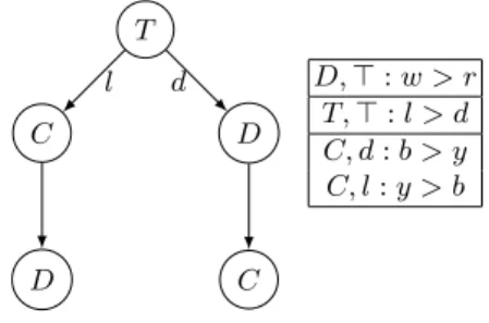
T D d C C l D D,⊤ : w > r T,⊤ : l > d C, d: b > y C, l: y > b

Fig. 1. Graphical representation of lexicographic orderings for Example 1

Example 1. Consider three attributes C(olor) with two values y(ellow) and b(lack), D(vd device) with two values w(riter) and r(ead-only), and T (ype) with values l(aptop) andd(deskop). The LP-structure σ depicted on Fig. 1 is a model for preferences about computers, where the type of computer is the most important criteria, with laptops al-ways preferred to desktops, and where the second criterium is color in the case of lap-tops, with yellow laptops preferred to black ones, whereas the second criterium is the type of optical drive in the case of desktops. In any case, a writer is always preferred to a read-only drive. The color is third criteria for desktops, with black preferred to yellow in this case.

The semantics of LP-structures is defined by the associated orderings over out-comes:

Definition 5. LP-structureσ = (T, P ) defines a partial strict order >σ over the set of outcomes as follows: given any pair of outcomes{α, β}, go down the tree, starting at the root, following edges that correspond to assignments made inα and β, until the

first noden is reached that is labelled with attribute X such that α(X) 6= β(X); we say thatn decides {α, β}. If there is a rule X, v :> in P that is applicable at n given u = α(Anc(n)) = β(Anc(n)), then α >σβ if and only if α(X) > β(X). If there is no rule that is applicable atn given u, or if no node that decides {α, β} is reached, α and β are σ-incomparable.

Example 1 (continued). According toσ, the most preferred computers are yellow lap-tops with a DVD-writer, becauseywl >σ α for any other outcome α 6= ywl; for any x ∈ C and any z ∈ D xzl >σ xzd, that is, any laptop is preferred to any desktop computer. Andywd >σbrd, that is, a yellow deskop with DVD-writer is preferred to a black one with DVD-reader because, although for desktops black is preferred to yellow, the type of optical reader is more important than the colour for desktop computers.

Proposition 1. Given a LP-structureσ = (T, P ), the relation >σ is irreflexive and transitive. It is also modular, i.e.,α >σβ implies either α >σ γ or γ >σβ. Moreover, ifσ is complete, then >σis a linear order.

The above proposition is saying>σ is a modular strict partial order. Every such order can be seen as the strict version of a total preorder. This means that even when >σ is not a linear order, it may still be viewed as “ranking” the different outcomes, with outcomes which areσ-incomparable given the same rank. (To be more precise, the relation≥σ defined byα ≥σ β iff [α >σ β or α, β are σ-incomparable] is a total preorder.)

2.2 Classes of lexicographic preference structures

Classes of structures with conditional preferences It should be clear that any

LP-structureσ is equivalent to a LP-structure σ′ _{where each edge corresponds to exactly} one value of its parent node, and where each preference rule applies to exactly one node: σ′ _{can be obtained fromσ by multiplying the edges that correspond to more than one} value; and by multiplying the preference rules that apply at more than one node. This structureσ′_{can be seen as a canonical representation of>σ. This leads to the following} defnition:

Definition 6. A CP&I LP-structure, or structure with conditional local preferences and

conditional attribute importance, is a structure in which each edge of the tree is labelled with a singleton value, and such that for each noden, that corresponds to exactly one partial assignmentu, the preference table contains one rule of the form X, u :> where X is the attribute that labels n.

CP&I LP-structures are particular cases of Wilson’s “Pre-Order Search Trees” (or POST) (2006): in POSTs, the preference relation at every node can be a non strict relation.

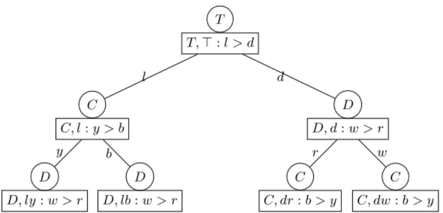
Example 1 (continued). A CP&I structure equivalent to the LP-structure depicted on Fig. 1 for Example 1 is depicted on Fig. 2. Note that when we draw a CP&I LP-structure, since local preferences at a given node can only depend on attributes above that node, we can represent the local preference relation corresponding to a node inside the node itself.

T T,⊤ : l > d C l C, l: y > b D y D, ly: w > r D b D, lb: w > r D d D, d: w > r C r C, dr: b > y C w C, dw: b > y

Fig. 2. A CP&I structure equivalent to that of Example 1

Another interesting class is that of structures with conditional preferences but uncon-ditional attribute importance:

Definition 7. A CP-UI LP-structure, or structure with conditional local preferences

and unconditional attribute importance, is a structure in which the tree is linear, with each edge labelled with the full domain of the attribute at the parent node, and such that for each noden, for each partial assignment u ∈ n, the preference table contains one rule of the formX, u :> where X is the attribute that labels n.

Classes of LP-structures with unconditional preferences We now turn to

lexico-graphic preferences with unconditional preferences, like the ones studied by e.g. Schmitt & Martignon (2006); Dombi et al. (2007); Yaman et al. (2008):

Definition 8. UP&I LP-structures, or structures with unconditional local preferences

and unconditional attribute importance, are structures whose attribute importance tree is linear, each edge being labelled with the full domain of the attribute at the parent node, and whose preference table contains one unconditional rule of the formX, ⊤ :> for each attributeX that appears in the tree. UP-CI LP-structures, or structures with unconditional local preferences and conditional attribute importance, are structures in which each edge of the tree is labelled with a singleton value, so that each node corresponds to exactly one partial assignment, but such that for each attribute that appears in the tree, the local preference table contains only one unconditional rule of the formX, ⊤ :>.

We can also define classes of LP-structures with unconditional, fixed preferences:

Definition 9. Given a non ambiguous setP of preferences rules, FP-UI(P ) is the class of UP&I structures that haveP for preference table. Similarly, FP-CI(P ) is the class of UP-CI structures that haveP for preference table.

3

Sample complexity of some classes of LP-structures

Our aim in this paper is to study how we can learn a LP-structure that fits well some examples of comparison. We assume a setE of examples, that is, of pairs of outcomes overA: we would like to find a LP-structure that is “consistent” with the examples in the following sense:

Definition 10. LP-structure σ is said to be consistent with example (α, β) ∈ A2 if α >σβ; σ is consistent with set of examples E if it consistent with every example of E. The problem of learning a structure that orders “well” the examples can be seen as a problem of classification: givenσ we can define another binary relation ≤σoverA

2 as follows:

α ≤σβ if and only if β >σα or (α 6>σβ and β 6>σ α).

Because >σ is modular,≤σ defined in this way is a total preorder overA (i.e. the relation is reflexive, transitive, and for everyα, β ∈ A, at least one of α ≤σβ or β ≤σα holds), and {≤σ, >σ} is a partition of A2

. In particular, we can define the Vapnik-Chernovenkis dimension of a class of LP-structures as the size of the biggest set of pairs (α, β) that can be “classified” correctly by some LP-structure in the class, whatever the labels (> or ≤) associated with each pair. In general, the higher this dimension, the more examples will be needed to correctly identify a LP-structure.

Proposition 2. The VC dimension of any class of transitive relations over a set of

bi-nary attributes is strictly less than2n .

Proof (Sketch). Follows from the fact that any graph with2n

vertices and2n edges contains at least one cycle, so that no class of transitive binary relations can shatter a set of2n

examples overA.

Proposition 3. The VC dimension of both classes of CP&I LP-structures and of CP-UI

structures overn binary attributes, is equal to 2n − 1.

Proof (Sketch). It is possible to build an AI tree overn attributes with 2k

nodes at the k − th level, for 0 ≤ i ≤ n − 1, with |n| = 1 for every node: this is a tree for CP&I structures, it has2n

− 1 nodes. Such a tree can shatter a set of 2n

− 1: take one example for each node, the local preference relation that is applicable at each node can be used to give both labels to the corresponding example. The upper bound follows from Prop. 2.

This result is rather negative, since it indicates that a huge number of examples would in general be necessary to have a good chance of closely approximating an un-known target relation. This important number of necessary examples also means that it would not be possible to learn in reasonable - that is, polynomial - time. However, learn-ing CP&I LP-structures is not hopeless in practice: decision trees have a VC dimension of the same order of magnitude, yet learning them has had great success experimentally. As for structures with unconditional preferences, Schmitt & Martignon (2006) have shown that hhe VC dimension of UP&I structures overn binary attributes is exactly n. Since every UP&I structure is equivalent to a CP-UI one, the VC dimension of UP&I structures overn binary attributes is at least n.

4

Preference elicitation/active learning

We now turn to a the active learning of preferences. The setting is as follows: there is some unknown target preference relation>, and a learner wants to learn a representa-tion of it by means of a Lexicographic Preference structure. There is a teacher, a kind of oracle to which the learner can submit queries of the form{α, β} where α and β are two outcomes: the teacher will then reply wetherα > β or β > α is the case. An important question in this setting is: how many queries does the learner need in order to completely identify the target relation>? More precisely, we want to find the commu-nication complexity of preference elicitation, i.e., the worst-case number of requests to the teacher to ask so as to be able to elicit the preference relation completely, assuming the target can be represented by a model in a given class. The question has already been answered in Dombi et al. (2007) for the FP-UI case. Here we identify the communi-cation complexity of eliciting lexicographic preferences structures in all 5 other cases, when all attributes are binary. (We restrict to the case of binary attributes for the sake of simplicity. The results for nonbinary attributes would be similar.) We know that a lower bound of the communication complexity is thelog of the number of preference relations in the class. In fact, this lower bound is reached in all 6 cases:

Proposition 4. The communication complexities of the six problems above are as

fol-lows, when all attributes are binary.

FP UP CP

UIlog(n!) Dombi et al. (2007) n + log(n!) 2n

− 1 + log(n!) CI g(n) = n −1 P k=0 2k log(n− k) n+ g(n) 2n − 1 + g(n)

Proof (Sketch). In the four cases FP-UI, UP&I, FP-CI and UP-CI,T and P are inde-pendent, i.e., anyP is compatible with any T . There are n! unconditional importance trees, andQn−1k=0(n − k + 1)2k

conditional ones. Moreover, when preferences are not fixed, there are2n

possible unconditional preference tables. For the CP-CI case, a com-plete conditional importance tree containsPn−1k=02

k = 2n

− 1 nodes, and at each node there are two possible conditional preference rules. The fact that these lower bounds are reached (in all 5 cases for which this has not been proved by Dombi et al. , 2007), we can explicit an elicitation protocol that guarantees to identifiy the preference structure.

5

Model identifiability

We now turn to the problem of identifying a model of a given classC, given a set E of examples: each example is a pair(α, β), for which we know that α > β for some target preference relation>. The aim of the learner is to find some LP-structure σ in C such thatα >σβ for every (α, β) ∈ E.

Dombi et al. (2007) have shown that the corresponding decision problem for the class of binary LP-structures with unconditional importance and unconditional, fixed lo-cal preferences can be solved in polynomial time: given a set of examplesE and a set P of unconditional local preferences for all attributes, is there a structure inFP − UI(P )

Algorithm 1 GenerateLPStructure

INPUT: A: set of attributes; E: set of examples over A; P : set of local preference rules: initially empty,

or contains a set of unconditional preference rules for the FLP cases; OUTPUT: LP-structure consistent withE, that contains P , or FAILURE;

1. T← {unlabelled root node};

2. while T contains some unlabelled node: (a) choose unlabelled node n of T ;

(b) (X, newRules)← chooseAttribute(E(n), Anc(n), P );

(c) if X= FAILURE then STOP and return FAILURE;

(d) label n with X; (e) P← P ∪ newRules;

(f) L← generateLabels(E(n), X); (Create set of labels for edges below n)

(g) for each l∈ L:

add new unlabelled node to T , attached to n with edge labelled with l; 3. return(T, P ).

that is consistent withE ? In order to prove this, they exhibit a simple greedy algo-rithm. We will prove in this section that the result still holds for most of our classes of LP-structures, except one.

5.1 A greedy algorithm

In order to prove this, we will prove that the greedy Algorithm 1, when given a set of examplesE, returns a LP-structure that satisfies the examples if one exists. The algo-rithm recursively constructs the AI-tree from the root to the leaves. At a given currently unlabelled node n, step 2b considers the set E(n) = {(α, β) ∈ E | α(Anc(n)) = β(Anc(n)) ∈ n} of examples that correspond to the assignments made in the branch so far and that are still undecided: it looks for some attributeX /∈ Anc(n) that can be used to order well examples inE(n) that can be ordered with X: there must be a set of local preferences rules of the formX, w :> that is not ambiguous when put together with the current set of rules, and such that for every(α, β) ∈ E(n), if α(X) 6= β(X) then there is a ruleX, w :> with w ⊆ α(U ) = β(U ) and α(X) > β(X). The attribute X can then be chosen for the label ofn, and the set of rules added to P . Step 2f then considers the values ofX that correspond to still undecided examples, and prepare labels that will be used for the edges fromn to its children. P is initially empty except in the case where the local preferences are known in advance, with only the order of importance to be learned. Note that this aproach cannot work in the case of conditional importance and unconditional preferences, as will be proved in Corollary 1.

Let us briefly describe the helper functions that appear in the algorithm:

generateLabels should return a set of disjoint subsets of the domain of the attribute at the current node; it takes as parameters a set of examplesE(n), and the attribute X at the current node: we require that for each example(α, β) ∈ E(n) that cannot be

decided atn because α(X) = β(X), there is one label returned by generateLabels that containsα(X).

We will use two particular instances of the function generateLabels: generateCondLabels(E, X) =

{{x} | x ∈ X and there is (α, β) ∈ E such that α(X) = β(X) = x}:

in the case of conditional importance, each branch corresponds to one value ofX. generateUncondLabel(E, X) = {X}: in the case of unconditional importance, one

branch is created, except that if there is no(α, β) ∈ E such that α(X) = β(X) = x, then generateUncondLabel(E, X) = ∅.

chooseAttribute takes as parameters the set of examplesE(n) that correspond to the node being treated, the set of attributes Anc(n) that already appear on the current branch, and the current set of preference rulesP ; it returns an attribute X not already on the branch ton and a set newRules of local preference rules over X: the attribute and the rules should be chosen so that they will decide well some examples ofE(n). More precisely, we will require that (X, newRules) is choosable with respect toE(n), Anc(n), P in the following sense:

Definition 11. Given a set of examplesE over attributes A, a set of attributes U ⊆ A and a set of local preference rules P , (X, newRules) is choosable with respect to E, U, P if X ∈ A − U , newRules is a set of local preference rules for X, and:

– P ∪ newRules is not ambiguous;

– for every(α, β) ∈ E, if α(X) 6= β(X) then there is a (unique) rule X, v :> in P ∪ newRules such that v ⊆ α(U ), and α(X) > β(X).

Moreover, we will say that(X, newRules) is:

UP-choosable if it is choosable andnewRules if of the form {X, ⊤ :>} (it contains a single unconditional rule);

CP-choosable if it is choosable andnewRules contains one rule X, u :> for every

u ∈ U such that there exists (α, β) ∈ E with α(U ) = β(U ) = u.

5.2 Some examples of GenerateLPStructure

In these examples we assume three binary attributes A, B, C. Throughout this sub-section we assume the algorithm checks the attributes for choosability in the order A → B → C. Furthermore we assume we are not in the FP case, i.e., the algorithm initialises with an empty local preference tableP = ∅.

Example 2. SupposeE consists of the following five examples:

1. (abc, a¯bc) 2. (¯a¯bc, ¯abc) 3. (ab¯c, a¯b¯c) 4. (¯a¯b¯c, ¯ab¯c) 5. (¯a¯bc, ¯ab¯c)

Let’s try using the algorithm to construct a UP&I structure consistent withE. At the root noden0of the AI-tree we first check if(A, newRules) is UP-choosable w.r.t. E, ∅, ∅. By the definition of UP-choosability, newRules must be of the form{A, ⊤ :>} for some total order> of {a, ¯a}. Now since α(A) = β(A) for all (α, β) ∈ E(n0) = E,

(A, {A, ⊤ :>}) is choosable for any >. Thus we label n0withA and add {A, ⊤ : a?¯a} toP , where “?” is some arbitrary order (< or >) over {a, ¯a}. Since we are working in the UP-case the algorithm then calls generateUncondLabel(E, A) = {a, ¯a} and gener-ates a single edge fromn0labelled with{a, ¯a} and leading to a new unlabelled node n1. The examplesE(n1) corresponding to the next node will be just {(α, β) ∈ E | α(A) = β(A)} = E (i.e., no examples in E are removed).5 _{At the next noden1, withA now}

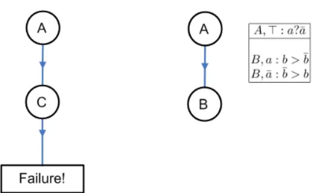
taken care of, we check if(B, newRules) is UP-choosable w.r.t. E(n1), {A}, P . We see that it is not UP-choosable, owing to the opposing preferences overB exhibited for instance in examples 1,2 ofE. However (C, {C, ⊤ : c > ¯c}) is UP-choosable, thus the algorithm labelsn1withC and adds C, ⊤ : c > ¯c to P . At the next node n2we have E(n2) = {(α, β) | α({A, C}) = β({A, C})} = {1, 2, 3, 4}. But the only remaining attributeB is not UP-choosable w.r.t. E(n2), {A, C}, P (because for instance we still have 1,2∈ E(n2)). Thus the sub-algorithm chooseAttribute(E(n2), {A, C}, P ) returns FAILURE and so does GenerateLPStructure in this case (see the left-hand side of Fig. 3). Hence there is no UP&I structure consistent withE.

However the algorithm does successfully return a CP-UI structure. This is because, at noden1, even though(B, newRules)is not UP-choosable w.r.t. E(n1), Anc(n1), P for any appropriate choice of newRules (i.e., of the formB, ⊤ :> in the UP-case), it is CP-choosable. Recall that to be CP-choosable, newRules must contain a ruleB, u :> for eachu ∈ n1 = {a, ¯a}, and in this case we may take newRules = {B, a : b > ¯b, B, ¯a : ¯b > b}. After this, since there is no (α, β) ∈ E(n1) such that α(B) = β(B), generateUncondLabel(E(n1), B) generates no labels and the algorithm terminates with the CP-UI structure on the right-hand side of Fig. 3.

Fig. 3. Output structures for Example 2. Left: The output is failure for UP&I structures. Right: The output CP-UI structure.

5_{Note in fact A is really a completely uninformative choice here, since it does not decide any} of the examples. A sensible heuristic for the algorithm - at least in the UP case - would be to disallow choosing any attribute X such that α(X) = β(X) for all examples. Such heuristics

Example 3. Consider the following examples:

1. (ab¯c, abc) 2. (abc, a¯bc) 3. (ab¯c, a¯b¯c) 4. (¯a¯bc, ¯ab¯c) 5. (¯abc, ¯a¯b¯c)

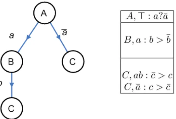
We will now use the algorithm to check if there is a CP&I structure consistent with these examples. We start at the root node n0, and check whether (A, newRules) is CP-choosable w.r.t.E, ∅, ∅. As in the previous example, since α(A) = β(A) for all (α, β) ∈ E, we may label n0withA, and add preference rule A, ⊤ : a?¯a to P , where “?” is some arbitrary preference betweena, ¯a. Since we are now in the CI-case, algorithm generateCondLabels(E, A) is called, which generates an edge-label for each value x of A such that α(A) = β(A) = x for some (α, β) ∈ E, in this case both a (see, e.g., example 1 in E) and ¯a (see, e.g., example 4). Thus two edges from n0 are created, labelled witha, ¯a resp., leading to two new unlabelled nodes n1andm1.

Following the right-hand branch leading tom1first (see Fig. 4), we haveE(m1) = {(α, β) ∈ E | α(A) = β(A) = ¯a} = {4, 5}. Here we first check if (B, newRules) is CP-choosable w.r.t.E(m1), {A}, P . By definition of CP-choosable newRules must be of the form{B, ¯a :>}. However due to the opposing preferences on their restriction to B exhibited by 4,5, we see there is no possible choice for > here. Thus we have to con-siderC instead. Here we see (C, {C, ¯a : c > ¯c}) is CP-choosable, thus m1is labelled withC, and C, ¯a : c > ¯c is added to P . Since generateCondLabel(E(m1), C) = ∅, no new nodes are created on this branch.

Now, moving back ton0 and following the left-hand branch to noden1, we have E(n1) = {(α, β) ∈ E | α(A) = β(A) = a} = {1, 2, 3}. Checking B for CP-choosability first, we see(B, {B, a : b > ¯b}) is CP-choosable w.r.t. E(n1), {A}, P , thus n1is labelled withB and B, a : b > ¯b added to P ; generateCondLabel(E(n1), B) = {{b}}, thus one edge is generated, labelled with b, leading to new node n2withE(n2) = {(α, β) ∈ E | α({A, B}) = β({A, B}) = ab} = {1}. For the last remaining attribute C on this branch we have (C, {C, ab : ¯c > c}) is CP-choosable w.r.t. E(n2), {A, B}, P . Thus the algorithm successfully terminates here, labellingn2withC and adding C, ab : ¯

c > c to P . The constructed CP&I structure in Fig. 4 is thus consistent with E.

5.3 Complexity of model identification

The table in Fig. 5 gives the parameters for the greedy algorithm that solve five learning problems. In fact, the only problem that cannot be solved with this algorithm, as will be shown below, is the learning of a UP-CI structure without initial knwoldge of the preferences.

Proposition 5. Using the right type of labels and the right choosability condtion and

the right initial preference table, the algorithm returns, when called on a given setE of examples, a structure of the expected type, as described in the table of Fig. 5, consistent withE, if such a structure exists

learning problem choosability labels initial P structure type CP&I CP-choosable conditional ∅ CP&I CP-UI CP-choosable uncond. ∅ CP-UI UP&I UP-choosable uncond ∅ UP&I FP-CI UP-choosable conditional 1 rule/attr. UP-CI FP-UI UP-choosable uncond 1 rule/attr. UP-CI Fig. 5. Parameters of the greedy algorithm for five learning problems

Proof (Sketch). The fact that the structure returned by the algorithm has the right type, depending on the parameters, and that it is consistent with the set of examples is quite straightforward. We now give the main steps of the proof of the fact that the algorithm will not return failure when there exists a structure of a given type consistent withE.

Note first that given any noden of some LP-structure (T, P ), labelled with X, if PX denotes the set of rules that are applicable atn with respect to any u ∈ n, then (X, PX) is clearly choosable with respect to E(n), Anc(n) and P′the set of rules that are applicable at some node not in the subtree belown. So if we know in advance some LP-structure(T, P ) consistent with a set E of examples, we can always construct it using the greedy algorithm, by choosing the "right" labels at each step.

Importantly, it can also be proved that if at some noden we choose another attribute X that is choosable, then there is some other LP-structure (T′_{, P}′_{), of the same type as} (T, P ), that is consistent with E and extends the current one; more precisely, (T′_{, P}′₎ is obtained by modifying the subtree ofT rooted at n, taking up X to the root of this subtree. Hence the algorithm cannot run into a dead end. This does not work in the UP-CI case, because taking an attribute upwards in the tree may require using a distinct preference rule, which may not be correct in other branches of the AI tree.

Corollary 1. The problems of deciding if there exists a LP-structure of a given class

consistent with a given set of examples over binary attributes have the following com-plexities:

FLP ULP CLP

UI P(Dombi et al. , 2007) P P

Proof (Sketch). For the CP&I, CP-UI, FP-CI, FP-UI and UP&I cases, the algorithm runs in polynomial time because it does not have more than|E| leaves, and each leaf cannot be at depth greater thann; and every step of the loop except (2b) is executed in linear time, whereas in order to choose an attribute, we can, for each remaining attribute X, consider the relation {(α(X), β(X)) | (α, β) ∈ E(n)} on X: we can check in polynomial time if it has cycles, and, if not, extend it to a total strict relation overX.

For the UP-CI case, one can guess a set of unconditional local preference rulesP , of size linear in n, and then check in polynomial time (FP-CI) case if there exists a attribute importance treeT such that (T, P ) is consistant with E; thus the problem in

NP. Hardness comes from a reduction fromWEAK SEPARABILITY – the problem of checking if there is a CP-net without dependencies weakly consistent with a given set of examples – shown to be NP-complete by Lang & Mengin (2009).

5.4 Complexity of model approximation

In practice, a general problem in machine learning is that there is often no structure of a given type that is consistent with all the examples at the same time. It is then interesting to find a structure that is consistent with the most examples. Schmitt & Martignon (2006) have shown that finding a UI&LP-structure, with a fixed set of local preferences, that satisfies as many examples from a given set as possible, is NP-complete, in the case where all attributes are binary. We extend these results here.

Proposition 6. The complexities of finding a LP-structure in a given class , which

wrongly classifies at most k examples of a given set E of examples over binary at-tributes, for a givenk, are as follows:

FLP ULP CLP

UI NP-completeSchmitt & Martignon (2006) NP-complete NP-hard

CI NP-complete NP-complete NP-complete

Proof (Sketch). These problems are in NP because in each case a witness is the LP-structure that has the right property, and such a LP-structure need not have more nodes than there are examples. For the UP-CI case, the problem is already NP-complete fork = 0, so it is NP-hard. NP-hardness of the other cases follow from successive reductions from the case proved by Schmitt & Martignon (2006).

6

Conclusion and future work

We have proposed a general, lexicographic type of models for representing a large fam-ily of preference relations. We have defined six interesting classes of models where the attribute importance as well as the local preferences can be conditional, or not. Two of these classes correspond to the usual unconditional lexicographic orderings, and to a variant of Wilson’s “Pre-Order Search Trees” (or POST) (2006). Interestingly, classes where preferences are conditional have an exponentional VC dimension.

We have calculated the cardinality of five of these six classes, and proved that the communication complexity for each class is not greater than thelog of this cardinality, thereby generalizing a previous result by Dombi et al. (2007).

As for passive learning, we have proved that a greedy algorithm like the ones pro-posed by Schmitt & Martignon (2006); Dombi et al. (2007) for the class of uncondi-tional preferences can identify a model in another four classes, thereby showing that the model identification problem is polynomial for these classes. We have also proved that the problem is NP-complete for the class of models with conditional attribute im-portance but unconditional local preferences. On the other hand, finding a model that minimizes the number of mistakes turns out to be NP-complete in all cases.

Our LP-structures are closely connected to decision trees. In fact, one can prove that the problem of learning a decision tree consistent with a set of examples can be reduced to a problem of learning a CP-CI LP structure. There remains to see if CP-CI structures can be as efficiently learnt in practice as decision trees.

In the context of machine learning, usually the set of examples to learn from is not free of errors in the data. Our greedy algorithm is quite error-sensitive and therefore not robust in this sense; it will even fail in the case of a collapsed version space. Ro-bustness toward errors in the training data is clearly an important property of real world applications.

As future work, we intend to test our algorithms, with appropriate heuristics to guide the choice of variables a each stage. A possible heuristics would be the mistake rate if some unconditional structure is built below a given node (which can be very quickly done). Another interesting aspect would be to study mixtures of conditional and uncon-ditional structures, with e.g. the first two levels of the structure being conuncon-ditional ones, the remaining ones being unconditional (since it is well-known that learning decision trees with only few levels can be as good as learning trees with more levels).

Acknowledgements We thank the reviewers for helpful comments. We even borrowed from them some of the sentences in this concluding section.

References

Booth, Richard, Chevaleyre, Yann, Lang, Jérôme, Mengin, Jérôme, & Sombattheera, Chattrakul. 2009. Learning various classes of models of lexicographic orderings. Tech. rept. Institut de Recherche en Informatique de Toulouse.

Boutilier, Craig (ed). 2009. Proceedings of the 21st International Joint Conference on Artificial Intelligence (IJCAI’09).

Dimopoulos, Yannis, Michael, Loizos, & Athienitou, Fani. 2009. Ceteris Paribus Pref-erence Elicitation with Predictive Guarantees. In: Boutilier (2009).

Dombi, József, Imreh, Csanád, & Vincze, Nándor. 2007. Learning Lexicographic Or-ders. European Journal of Operational Research, 183, 748–756.

Koriche, Frédéric, & Zanuttini, Bruno. 2009. Learning conditional preference networks with queries. In: Boutilier (2009).

Lang, Jérôme, & Mengin, Jérôme. 2009. The complexity of learning separable ceteris paribus preferences. In: Boutilier (2009).

Schmitt, Michael, & Martignon, Laura. 2006. On the Complexity of Learning Lexico-graphic Strategies. Journal of Machine Learning Research, 7, 55–83.

Wilson, Nic. 2006. An Effcient Upper Approximation for Conditional Preference. In: Brewka, Gerhard, Coradeschi, S., Perini, A., & Traverso, P. (eds), Proceedings of the 17th European Conference on Artificial Intelligence (ECAI 2006).

Yaman, Fusun, Walsh, Thomas J., Littman, Michael L., & desJardins, Marie. 2008. Democratic Approximation of Lexicographic Preference Models. In: Proceedings of the 25th International Conference on Machine Learning (ICML’08).