Cumulative Prospect Theory, employee exercise
behaviour and stock options cost assessment
Hamza BAHAJI ∗
Université de Paris Dauphine, DRM Finance
December 2011
Abstract
This research provides an alternative framework for the valuation of standard employee stock options and for the analysis of exercise behavior patterns. It develops a binomial model where the exercise decision obeys to a policy that maximizes the expected utility to a representative employee exhibiting preferences as described by the Cumulative Prospect Theory (CPT). This model also accounts for exogenous non-market factors that may cause early exercise. Using a large database on stock options exercise transactions in 12 US public corporations, we examined the performance of our model in predicting actual exercise patterns. Interestingly, the model calibrations yield probability weighting coefficient estimates that are consistent with the estimates from the experimental literature. Further, our results suggest that the CPT-based model outperforms the Expected Utility Theory-based model in predicting actual exercise patterns in our sample. These findings convey the main contribution of this paper which is the strong ability of the CPT framework to explain the employees exercise behavior. It therefore provides rationale for using this framework in order to get more accurate fair value estimates of employee stock options contracts.
JEL Classification:G13, G30, J33, M41.
Keywords:Stock options, Exercise behavior, Cumulative Prospect Theory, Fair value, Option valuation.
∗
DRM- Finance, Université de Paris Dauphine, Place du Général du Lattre de Tassigny, 75 775, Paris Cedex 16, France. E-mail:
1.
Introduction
The extensive use of stock options in employee compensation packages and their increasing popularity as long term incentives tools have brought many of their corporate issues at the forefront of public debate. Professionals and regulators have become specifically concerned about assessing their cost to shareholders. This issue has been intensified by the requirements of accounting standards (IFRS and US GAAP) from public companies to fairly recognize the cost of stock options grants. Thus suitable expensing of employee stock options has become a focus of attention in financial accounting.
The complexity with the assessment of the stock options fair value is that their payoffs depend on the exercise behavior of the holder employee. This behavior deviates from the usual value-maximizing exercise policy stated by the standard American option theory because of many reasons. First, opposite to ordinary tradable call options, employee stock options are long-dated nontransferable1 call options. This implies that the employee has to bear the underlying risk for a long time. Second, the employee faces hedging restrictions since he is precluded from short selling the company’s stock. Finally, employee holding stock options may be unable to completely diversify his stock holdings and human capital investment in the firm. Because of these features, the employee will not make the same exercise decision as an unrestricted outside investor. Therefore, the fair value of a stock option contract crucially depends on the holder employee endowment and risk preferences patterns.
Given that the values of employee stock options are unobservable, their valuation requires a theoretical modeling of the exercise policy of the holder employee. There is an extensive literature focused on this issue. Most of it relies on the Expected Utility Theory (EUT henceforth) to develop utility-maximizing binomial models (Huddart, 1994; Markus and Kulatilaka, 1994; Carpenter, 1998…). These approaches consider that the employee chooses an optimal exercise decision as part of a utility maximization problem that may simultaneously cover other issues such as consumption and portfolio choices (Detemple and Sundaresan, 1999), non-option wealth diversification or liquidity needs. Nonetheless, these models specifically rely on the validity of the underlying theoretical framework, namely the EUT.
Beyond the well known limitations of the standard normative model in explaining some patterns of economic agent behavior, it has shown handicaps in capturing some prominent features of employee equity-based compensation. For instance, EUT-based models, taking place in principal-agent framework, have difficulties accommodating the existence of convex contracts as part of the
1 Market experience shows however some exceptions to this feature, such like the transferable stock options programs developed by JP Morgan Chase for Microsoft in July 2003 and for Comcast in September 2004. According to this deal, JP Morgan offers the entitled employees to purchase their underwater stock options at a discount premium (i.e. below their potential market value).
executive compensation package2. Consistently, studies focused on the effect of stock option and restricted stock grants on managerial effort incentives, such like Jenter (2001), Hall and Murphy (2002) and Henderson (2005), conclude that stock options are inefficient tools for creating incentives for risk-averse managers when they are granted by mean of an offset of cash compensation. This is obviously inconsistent with actual compensation practices. Moreover, a common prediction of the EUT-based models is that a risk-averse undiversified employee would value his options below their risk-neutral value (Lambert et al., 1991; Hall and Merphy; 2000, 2002; Henderson, 2005…), which contrasts to several surveys and empirical findings documenting that, frequently, employees are inclined to overestimate the value of their stock options compared to the theoretical fair market value (Lambert and Larcker, 2001; Hodge et al., 2006; Hallock and Olson, 2006; Devers et al., 2007). Furthermore, there is an empirical evidence on employees decisions, and specifically those related to the exercise of their stock options (Huddart and Lang, 1996 ; Heath et al., 1999), being driven by psychological and behavioral factors that are out of the scope of the EUT. Actually, these limitations of the EUT framework provide rationale and motivation for investigating the ability of an alternative theoretical framework to better predict employee stock option exercise patterns.
This paper develops a stock option exercise and valuation binomial model where the exercise decision obeys to a policy that maximizes the expected utility of a representative employee exhibiting preferences as described by Tversky’s and Kahneman’s (1992) Cumulative Prospect Theory (CPT hereafter). This model also accounts for exogenous non-market factors that may cause early exercise through an exit state that occurs with a given probability. This research aims to provide an alternative framework for the valuation of employee standard stock options contracts and the analysis of exercise behavior patterns. The purpose of this work is also to contribute to a growing literature on employee equity-based compensation that incorporates CPT-based models. These models have proved successful in explaining some observed compensation practices, and specifically the almost universal presence of stock options in the executive compensation contracts. Therefore, they have advanced CPT framework as a promising candidate for the analysis of equity-based compensation contracts. This literature includes in particular Dittmann et al. (2010) who developed a stylized principal-agent model that explains the observed mix of restricted stocks and stock options in the executive compensation packages. It also includes Spalt (2008) who used the CPT framework, and especially the probability weighting feature, to prove that stock options may be attractive to a loss-averse employee subject to probability weighting. He then explained the puzzling phenomenon that riskier firms are prompted to grant more stock options to non-executive employees. This literature comprises also Bahaji’s (2011) research that elaborates on stock options incentives effect and some implications in terms of contract design aspects.
2
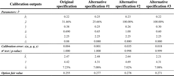
Further, I examined the performance of the CPT model in predicting actual exercise patterns in 12 US public firms over the period from 1985 to 2007. Specifically, I compared the model performance to those of two competing models, namely the EUT-based binomial model (EU model hereafter) introduced in Carpenter (1998) and the stopping-state American model (EA model in the reminder of the paper). The latter is a binomial version of Jennergren and Naslund (1993) continuous-time model. Given that some factors underlying the models are not observable, I calibrate the models on the average data from the sample using the calibration procedure in Carpenter (1998). The statistical significance tests show that the models fit the average data remarkably well. Interestingly, the base case calibration of the CPT model yielded an estimation of the probability weighting parameter that lies within the range of the experimental estimates. Next, I compared the performance of the parameterized models in predicting actual exercise patterns in the sample. I found that the CPT model brings a significant improvement over the EU model and the EA model in terms of both the size of the forecast errors and the explanatory power of the regressions. Even when relaxing the assumptions regarding the exogenous non-market factors, the CPT model yields slightly better forecasts compared to those of the EU model. Therefore, the CPT framework turns out to be the best candidate in explaining exercise patterns in the sample.
The last item discussed in this paper is the stock option fair value assessment. For the purpose of comparing the option faire value under each of the three competing models, I assessed the fair value of the stock option contract for the representative firm in the sample (i.e. the average firm). In addition, for the purpose of comparison with some methods recommended by the international accounting standards and largely indoctrinated by practitioners, I computed option fair values using two benchmark models. The first one is the extension of the Black & Scholes model (BS henceforth) that uses the expected lifetime of the option as an input instead of its contractual expiration date. The second benchmark is the Hull and White (2004) model. The results show that, on the one hand, the CPT model and the EU model yielded values are close (a difference of about 4%) and that, on the other hand, the values from the three models are significantly lower than the values computed based on the two benchmark approaches. Specifically, if we consider that the CPT model is the most accurate model in the sense that it predicts the best exercise patterns, we would admit that the benchmark models overestimate the value of the representative company’s stock option contract by 10% to 20%. Another finding from this analysis is that the models display different sensitivities to market factors, especially volatility and dividend yield. These sensitivities depend also on the models specifications.
The remainder of the paper is structured as follows. In the 1st section stock option exercise and valuation related literature is reviewed. The 2nd section sketches a theoretical framework for stock option exercise from the perspective of a CPT representative employee and describes, step-by-step, the construction of the CPT model and the implied exercise prediction statistics. This section also
provides some numerical analyses of the model sensitivity to the preferences-related factors. Section 3 presents the empirical analysis comparing the predictive power of the models regarding actual exercise patterns in a sample of 12 US firms in the NYSE and the NASDAQ. The last section discusses the stock option fair value estimates from the models.
2.
Stock option exercise and valuation: related literature
With the increasing interrogations surrounding the use of employee stock option, their exercise and valuation issues have become a focus of interest of a rapidly growing literature. This literature includes several empirical studies that attempted to bring the spotlight on the determinants of early exercise patterns. Hemmer et al. (1996), Core and Guay (2001) and Bettis et al. (2005) investigated economic/rational factors driving exercise decisions such as liquidity needs and risk diversification. Huddart and Lang (1996) studied the exercise behavior of over 50,000 employees at eight corporations. They mainly found that exercise is strongly associated with recent stock price movements. Heath et al. (1999) have found empirical evidence suggesting that psychological factors may also lead the employee to sacrifice some option value by exercising it early. Consistently, Bahaji (2009) showed that stock option exercise patterns in 12 US companies display myopic behavior denoting the well documented mental accounting behavioral bias. Sautner and Weber (2005) also provided some interesting empirical results suggesting that employees exercise decisions denote psychological bias, such as miscalibration and mental accounting. This line of studies also includes Core and Guay (2001), Misra and Shi (2005) and Armstrong et al. (2006). All these studies provide rationale for behavioral factors to be considered in a theoretical framework for employees exercise decisions.
One approach that has been suggested in the literature to address the problem of non-transferability and hedging restrictions effects on exercise behavior is to model the employee exercise policy relying on the EUT framework. These papers characterized the optimal exercise policy by a utility-maximization problem. Huddart (1994) and Kulatilaka and Marcus (1994) were the first to have introduced binomial models where the exercise occurs as soon as the utility from the exercise proceeds exceeds the expected utility from holding the option for another period, with non-option wealth invested in the risk-free asset. Carpenter (1998) extended this approach to take into account early exercise or forfeiture due to job termination, using an exogenous Poisson process with a given stopping rate3. Another improvement brought by Carpenter (1998) is the investment of the employee non-option wealth in the Merton optimal portfolio instead of the risk-free asset. She calibrated her model to mean exercise data from a sample of 40 US firms. She found that, surprisingly, the EU model performs almost as good as a simple extension of the usual binomial model including an
3 Papers that focused on the impact on the stock option fair value of forfeiture and early exercise due to job termination include Jennergren and Naslund (1993), Cuny and Jorion (1995) and Rubinstein (1995).
exogenous stopping state, which suggests that “exercise patterns can be approximately replicated
merely by imposing a suitable stopping rate, without the need to make assumptions about [...] risk aversion, diversification, and the value of new employment “. Detemple and Sundaresan (1999)
suggested an extension that allows for simultaneous portfolio choice and stock option exercise decisions. Bettis et al. (2005) built on Carpenter’s (1998) approach to carry out an analysis of exercise patterns within a sample of 140,000 option exercises by corporate executives at almost 4,000 firms. They calibrated the EU model to their median data. Their results contrast with those of Carpenter (1998) in that they show that the EU model outperforms the stopping state binomial model in forecasting exercise behavior.
Another line of studies has advocated an approach based on exogenous specification of the exercise policy. Rubinstein (1994) and Cuny and Jorion (1995) built stock option pricing models under exogenous assumptions about the exercise timing. Jennergren and Naslund (1993) and Carr and Linetsky (2000) derived analytical valuation formulas assuming exogenous specified forfeiture rates and exercise boundaries. Moreover, a paper by Hull and White (2004) proposed a binomial model assuming that vested options are exercised whenever the stock price hits an exogenous hurdle specified as a multiple of the stock price at inception. Their approach also allows for the possibility that the option holder might have to leave the firm for exogenous reasons and, therefore, needs to forfeit or exercise his options provided these are in-the-money. Relying on Hull’s and White’s approach, Cvitanic et al. (2004) provided an analytical pricing formula. However, Carpenter et al. (2010) showed that the optimal exercise policy needs not to be specified in the form of a single critical stock price boundary. They nevertheless proved under the risk-neutral probability measure the existence of a single stock price exercise boundary for CRRA utility functions with risk aversion coefficient less than or equal to one.
More recent literature has underscored the relevance of valuation approaches that proceed by using empirically estimated exercise hazard functions to describe the stock option’s expected payoff. Carpenter et al.(2006) suggested a method – similar to that used for the modeling of the prepayment of the mortgage-backed securities – relying on estimated exercise and cancellation rates as a hazard function of the stock price path, time to expiration and both firm and option holder characteristics. Armstrong et al.(2006) modeled exercise rates as a function of idiosyncratic behavioral and economic factors such as attainment of performance benchmarks, recent vesting, portfolio value, and employee rank. They proved that estimates from an idiosyncratic exercise rate model are also more accurate in predicting out-of-sample realized option values.
Finally, several researches have attempted to undertake the issues related to reloading and resetting features’ effect on stock options exercises and valuation (Hemmer et al., 1998; Saly et al.,
1999; Dybvig and Loewenstein, 2003…), whilst other studies have focused on valuation issues related to block exercise behavior (Henderson, 2006; Grasselli and Henderson, 2009).
3.
The CPT exercise model
This section develops a model of stock options exercise and valuation from the viewpoint of the issuer (i.e. the firm). The model is based on a theoretical framework where the option cash flows depend on the exercise behavior of a representative option holder whose risk preferences fit with the CPT framework. This section provides in addition some numerical analyses of the sensitivity of the model outputs to risk preferences parameters.
3.1.The economy of the stock option contract
The representative employee is assumed to be granted a stock option contract at time t=0 expiring within a time period “T”. The contract is a Bermudan style call option on the common stock of the company denoted by “St”, with strike price “K”. It includes two restrictions as commonly do standard employee stock options. The first one is the non-transferability, which means that the employee is precluded from selling the option. The second one is the vesting, which implies the Bermudan feature of the option. The vesting restriction requires the cancellation of the contract in case the holder leaves the company before the end of the vesting period “tv”. In addition, I assumed that the employee is not allowed to short-sell the company stock and that he can earn the risk-free rate “r” from investing in a riskless asset. Hence, this assumption stands for a restriction on the hedging of the option.
Moreover, the underlying is assumed to follow a standard CRR binomial process with “N” time steps. Thus, in each time step “δt=T N/ ” the stock price may move up by a factor “u=eσ δt” with a
probability “ ( ). / q t e u p u u µ− δ − = −1
” or down by factor “d=1/u”. “σ”, “µ” and “q” are the stock price volatility, the expected return and the dividend yield respectively. Note that the upward risk neutral
probability is given by: ( )
. * / r q t e u p u u δ − − = −1 .
Furthermore, following Carpenter (1998), I assumed that in each time period there is an exogenous probability “pe” for the employee to be offered a cash amount “y” per each option held to leave the company. Leaving the company implies that the option contract is stopped at that time either through exercise, provided the option is vested and is in-the-money, or forfeiture if not.
I assumed that the representative employee exhibits preferences as described by the CPT (Tversky and Kahneman, 1992). It follows that to each gamble “x” with countable outcomes “
x
i∈{1,...,n}” andtheir respective probabilities “
p
i∈{1,...,n}”, the employee assigns the value:( )
,( )
1 n a i i i V xω
vθ x = =∑
(1) Where the functionv
θ( )
.
, called the value function, is assumed of the form:( )
(
)
(
)
; ; y y v y y y α θ αθ
θ
λ θ
θ
− ≥ = − − < , where 0< ≤α
1andλ
≥1 (2)This formulation has some important features that distinguish it from the normative utility specification. The value function is defined on deviations from a reference point, denoted by “θ”. It is concave for gains (i.e. implying risk aversion) and commonly convex for losses (i.e. implying risk seeking) due to parameter “α”. It is steeper for losses than for gains (i.e. conveying a loss aversion feature caught up through “λ”).
The terms “
ω
a i, ” in (1) are decisions weights associated to each outcome. These result from a transformation of the probabilities using a weighting function “ψ
a( )
.
”. It applies to cumulative probabilities, represented by the cumulative probability function “F
( )
.
”, as follows:( )
(
)
(
( )
)
( )
(
)
(
( )
)
( )
1 1 1 , 1 1 1 1 1 ; ; n n a j a j a i a i i j i j i i i a i a j a j a i a i i j j a i p p F x F x x p p F x F x x p ψ ψ ψ ψ θ ω ψ ψ ψ ψ θ ψ − = = + − − = = − = − − − ≥ = − = − < ∑
∑
∑
∑
{ }
;i ,n = 1 (3)Following Tversky and Kahneman (1992), the probability weighting function is assumed of the form:
( )
(
)
1 (1 ) a a a a a p p p p ψ = + − where 0 . 2 7 9 < a ≤1 (4)This function stands for another piece of the CPT, which is the nonlinear transformation of probabilities. Specifically, it captures experimental evidence on people overweighting small probabilities and being more sensitive to probability spreads at higher probability levels. The degree of probability weighting is controlled separately over gains and losses by the weighting parameter “a”4. The more this parameter approaches the lower boundary 5 at 0.279 the more the tails of probability distribution are overweighted. For instance, when we set “a” to 1, probability weighting assumption is relaxed.
3.3. Setting up the CPT model
Using an alternative behavioral framework, the CPT model builds on prior works by Huddart (1994), Kulatilaka and Marcus (1994) and Carpenter (1998) in that it uses the same principle governing the exercise decision. Similar to these models, the CPT model is a two-state lattice where the optimal exercise decision is driven by the maximization of the expected utility from exercise proceeds. According to this maximization principle, the option is exercised in a given time period if the utility from the exercise proceeds at that time is higher than the expected utility from continuing to hold the option until the next time period. With that said, the representative employee is supposed to exercise as soon as the intrinsic value of the option exceeds the value of the option from his own perspective (i.e. the subjective value). However, opposite to these models, the utility is assessed using the CPT framework instead of the EUT. Therefore, the key differentiating point is that, on the one hand, only the utility of exercise proceeds is considered rather than that of total wealth and, on the other hand, the expected utility is assessed based on weighted reel probabilities.
3.3.1. Model construction
The first step of the CPT model construction consists in determining the weighted transition probabilities that will be used to assess the utility expectation at each node of the share price binomial tree. The purpose is to build in parallel to the share price binomial process a distorted/skewed two-state process that fits with the employee view of probabilities as specified by the CPT probability weighting function6 in (4). This process relies on a probability tree with the same share price nodes as
4 Actually, according to the CPT, the degree of probability weighting is controlled separately over gains and losses through two different weighting parameters, “a” and “b” respectively. For simplicity, I assumed these parameters to be equal (i.e. a=b).
5
The lower boundary at 0.279 is a technical condition to insure that “ a
( )
pp ψ ∂
∂ ” is positive over ]0,1[ as required
by the following first order condition: (a-1)pa + (a(1-p)+p)(1-p)a ≥ 0. This constraint insures that the probability
weighting function can not assign negative decision weights consistent with first order stochastic dominance. For farther details see Ingersoll (2008).
6 An interesting alternative to the CPT probability weighting function is to use weighting functions implied by listed options prices. This approach uses non-parametric methods to estimate state price densities from options
the binomial tree. The approach used to build this tree is described through the set of equations in appendix A1. As stated, this approach keeps the original share price nodes unchanged and uses forward induction to recover all transition probabilities starting from the root of the tree.
The second step in building the model is about setting the patterns of exercise decision. Following Carpenter (1998), I accommodate the possibility of option forfeitures or early exercises caused by non-market events, such as liquidity shocks, employment termination or any other forced exercise through the exit states. Note that the exit decision is an endogenous feature of the model in that it is linked to the size of the cash amount “y” offered to the employee to leave. In addition, I assumed that the exercise decision in a given time period depends on whether or not the exit state is prevailing at that time, the vesting status of the option and the prevailing level of stock price, but not the past stock price path. This assumption allows for backward recursion approach.
Moreover, as stated in assumption 1 bellow, the employee is supposed to set his reference point based on his initial own share price return expectations over the lifetime of the option:
Assumption 1: the reference point “
θ
i” at a time period “ti” is defined as the intrinsic valueresulting from a time-adjusted growth rate of the share price based on the annualized return “
ρ
”reflecting the expectations of the employee:
( )
(
q i t)
i Se K ρ δθ
= − − + (5)While this setting is inconsistent with empirical evidence on employee exercise activity being linked to share price historical maxima (Huddart and Lang, 1996; Heath et al, 1999; Bahaji, 2009), it nevertheless conveys an exercise behavior taking into account non-status quo reference points. Actually, under a path-dependent specification of the reference point, backward recursion becomes impossible in our situation. The specification in (5) is also supported by Hodge et al. (2006) findings that employees usually use heuristics to attach values to their stock options, like determining the intrinsic value from their expectations about future stock price. Recall that although the CPT specifies the shape of the value function around the reference point, it does not provide guidance on how people set their reference points. Neither does most of the psychological literature relying on the assumption according to which the reference point is the Status quo. Instead, this literature admits both the existence and the importance of non-status quo reference points since “there are situations in which
gains and losses are coded relative to an expectation or aspiration level that differs from the status
market prices. These estimates are then used as building blocks to construct non-parametric estimators of the weighting function without imposing any constraint on the shape of the former. For more details on this approach see Polkovnichenko and Zhao (2009).
Notation
• h : Intrinsic value of the option i j,
at note (i,j).
• p : Weighted transition i j,
probability at node (i,j).
• p∗ : Risk neutral transition probability at node (i,j).
• Ce : Subjective value of the i j,
option at node (i,j) determined based on the certainty equivalence principle.
• C : Risk-neutral value of the i j,
option at node (i,j).
• 0 , i j
V : Continuing state exercise decision outcome at node (i,j).
• 1 , i j
V : Exit state exercise decision outcome at node (i,j).
• θi: Reference point at the i
th
level of the tree.
Figure-1: Illustration of the CPT model construction.
This figure exhibits the structure of the CPT model tree at node (i,j). The upper branches represent the exit state. Equation (5.1) formulates the exercise outcome related to that state. Equation (5.2) gives the exercise outcome at the continuing state represented by the lower branches. Equations (5.3) and (5.4) provide, respectively, the option risk neutral value and subjective value.
(5.4) ( ) { } {( ) } 1 , , , , , , , 1I 1I i j i j hi jy Cei j i j hi j y Cei j V C h + ≤ + > = + { } { } 0 , , , , , , , 1I 1I i j i j hi jCei j i j hi jCei j V =C ≤ +h >
(
)
(
0 0) (
1 1)
, 1 1, 1 (1 ) 1, 1, 1 (1 ) 1, r t i j e i j i j e i j i j C = −p p V∗ + + + −p V∗ + +p p V∗ + + + −p V∗ + e−δ(
)
(
(
)
( )
)
(
(
)
( )
)
1 0 0 1 1 , 1 , 1 1, 1 (1 ,) 1 1, , 1 1, 1 (1 ,) 1 1, r t i j i e i j i i j i j i i j e i j i i j i j i i j Ce =vθ− −p p vθ+ V+ + + −p vθ+ V+ +p p vθ+ V+ + + −p vθ+ V+ e−δ Continuing state 1−pe e p 1 1, 1 i j V+ + 1 1, i j V+ , i j p , 1−pi j (5.1) (5.2) (5.3) Exit state 0 1, 1 i j V+ + 0 1, i j V+ , i j p , 1−pi jquo” (Kahneman and Tversky, 1979). Research on the Disposition Effect7 has paid greater attention to
this issue (Shefrin and Statman, 1985; Heisler, 1998; Odean, 1998a). These studies have found strong evidence on reference points being set in a dynamic fashion. Moreover, literature on reference point adaptation is still developing. This literature includes few papers such as Koszegi and Rabin (2006) and Yogo (2005) that posit that people set their reference point based on their expectations about the future instead of the starting point (ex: original purchase price). It also includes researches that provided experimental evidence on people using historical maxima as reference points (Gneezy, 1998), shifting their reference points after a stimulus is presented (Chen and Rao, 2002) and adapting them asymmetrically more completely over gains than over losses (Arkes et al.; 2006).
Finally, I made the following assumption regarding block exercise (i.e. policy of spreading exercise over several separate transactions) that implies that the exercise in the CPT model is an “all
or nothing” exercise policy:
Assumption 2: when the employee decides to exercise, he will do so for all his outstanding options at
once in a single block provided these options are part of the same grant and, therefore, have the same characteristics.
7 Disposition effect is a term coined by Shefrin and Statman (1985) to refer to the tendency of individual investors to hold loser stocks and sell winner stocks defined relative to a purchase price reference point.
Figure-1 exhibits the construction of the model at the jth node of the ith level of the tree (i.e. at time “ti =i t.
δ
”) denoted by (i,j). The option is assumed to have already vested at that level. As illustrated, the exercise decision relies on the subjective value of the option considering four states of the world (i.e. stopping/continuing states combined with upward/downward sates). The latter is assessed over these four states based on the certainty equivalence principle using the weighted transition probabilities and the exit probability. Thus, in the continuing state, the option is exercised as soon as the intrinsic value exceeds the subjective value of the option. However, in the exit state, the employee decides to continue with the option if its subjective value is greater than the sum of its intrinsic value and the cash amount he is offered to leave the company. By repeating this process using backward recursion, starting from the end of the tree, we can find out the nodes where the option is exercised. Note that at the levels where the option is still unvested, it is systematically held to the next period provided the employee is in the continuing state. Nevertheless, unvested option is forfeited in the exit state if its subjective value is lower than the leaving-cash amount. A formal algorithm describing the discussed exercise rule is provided in the appendix A2.3.3.2. Model outputs and predictions
Similar to Carpenter (1998) and others, I considered that the employee exercise patterns are characterized by two main variables: the exercise stock price ratio, defined as the stock price-to-strike price ratio at the time of exercise, and the lifetime of the option, denoted respectively by “Sτ” and “
τ
”. It follows that the statistics of interest denoting the exercise patterns predictions implied by the model are the expectations of these two random variables subject to the final share price:(
*)
ˆ p | T Sτ =IE Sτ s (6)( )
* ˆ IEp |sT τ= τ (7)Where “
IE
p( )
. | .
” is the conditional expectation operator under the reel probability measure.Specifically, the expectations above are determined as the weighted average of the outcomes of the random variables “Sτ” and “
τ
” across all the stock price paths that result in an exercise and settle at a final stock price level “sT*”. Note that these predictions take into account the effect of the share price effective performance on the exercise behavior since they are conditioned on the terminal share price level. This makes them comparable to equivalent mean values from empirical data, which enables to test the model prediction power and to calibrate it (i.e. estimate the unobservable parameters of the model).The expected value of the cancellation rate ”
η
” is another model-yielded variable that has to be considered for the purpose of calibration on empirical data:( )
ˆ p
IE
η= η (8)
The estimation of this statistic consists in recursively computing the 1-year cancellation probability based on the implied distribution of the cancellation state variable across all share price paths. Therefore, it may be interpreted as the average ratio of cancelled options during a year either through forfeitures or expirations. Note that, opposite to the two previous statistics in (6) and (7), the mean cancellation rate is not conditioned on a final share price level. Let’s stress also that the cancellation rate has to be distinguished from the exit rate. The latter is the model input that drives the frequency of forfeitures prior to the expiry date, whereas the former is a model output that results from the implied exercise policy and, consequently, depends on the model parameters and especially the exit rate.
3.3.3. Model drawbacks
The CPT model assumes that when the employee decides to exercise he will do it for all his options at once. It therefore ignores the possibility of fractional exercise8 (i.e. the tendency of employees to exercise large quantities of options on a small number of occasions) in spite of its empirical evidence (Bahaji, 2009). In addition, the model do not account for tax constraints effect on exercise decision. Moreover, the influence of private information that may be held by the employee, as an insider, on his exercise behavior is left out as well. The model ignores also the potential dependence of the exercise policy of the employee on the compensation policy of the firm and vice versa. Finally, let’s emphasize that the model predictions are contingent to the validity of the underlying theoretical frame work (i.e. the CPT). In fact, since stock options subjective values are not observable, the obvious recourse is to rely on a theoretical framework in order to specify the exercise policy of a representative employee. If at least subjective values were observable for European call options, one could use them as building blocks to construct an implied share price lattice9. Actually, we can demonstrate in a continuous time setting, under some technical assumptions, the existence of a stock price diffusion process that is compatible with these subjective values (see appendix A3). This implied stock price diffusion allows reproducing all input subjective values and, therefore, integrates employee risk preferences patterns. Once discretized, using for instance lattice approaches, it could be used as an alternative for the valuation of standard employee stock options (i.e. Bermudan-style stock options).
8 Many authors have suggested models that take into account individual exercise as well as block exercise behavior: see for example Henderson (2006) and Carpenter et al.(2006).
9
3.4.Some numerical simulations
In order to provide a concrete outline on the profile of the outputs yielded by the model along with their respective sensitivities to some parameters of the model, in particular those specific to the CPT (i.e. preferences-related parameters), I performed numerical analyses based on a base case setting of the stock option contract conditions and the preferences parameters of the representative employee.
3.4.1. A numerical application
Consider the case of a representative employee who holds a 4-year at-the-money (ATM henceforth) stock option (T=4) vesting in a year (tv=1) with a strike price “K=1”. For the remaining option-related parameters, assume no dividend payments (q=0), a stock price volatility at “
σ
=30%”, a risk-free rate “r=3%” and an expected stock price return of “µ
=7%”. In addition, let’s set the curvature parameter of the value function “α
”, the probability weighting factor “a” and the loss aversion coefficient “λ
” at respectively 0.88, 0.64 and 2.25 based on the experimental estimates from the CPT (Tversky and Kahneman, 1992). Moreover, to calibrate the reference point function in (5), we will set the parameter “ρ” at 10%, which boils down to assuming that the representative employee assesses his gains and losses over the option holding period with respect to a share performance hurdle of 10% per annum. Finally, we will consider that, each year, the representative employee is offered an amount “y=0.30” to leave the company with a probability “ pe=0.25”.Panel-2 of figure-2 exhibits the standard CRR binomial stock price tree resulting from the setting
above. The share price upward and downward movers are generated by factors “e+σ δt ≈1.35” and “e−σ δt ≈0.74” respectively using yearly time step “
δ
t=1”. The risk-neutral transition probability at every node is “p∗ ≈0.475”. The yearly reel transition probability is “p≈0.545”. It implies the weighted transition probability tree displayed in Panel-1. As we can see, the weighted transition probability is increasing with the share price and tends to be higher than the reel transition probability at the upper nodes. This result conveys the well established phenomenon on individuals overweighting small probabilities. Given the profile of the weighted transition probabilities, the representative employee is expected to value his option in excess of its risk-neutral value at upper nodes. Therefore, he will delay exercise at these nodes. Actually, we can see this when looking at Panel-3 and Panel-4: the subjective values are higher than the risk neutral values at the upper nodes. To get a more concrete outlook on that, let’s focus on nodes A, B and C. The intrinsic value of the option at node A is “h3,3 ≈1.460” while the subjective value is “Ce3,3 ≈1.855”. At the continuing state, the employee will delay then the exercise since the option is worth, from his own perspective, much more than its intrinsic value. He will not exercise under the exit state neither because the exit amount is notFigure-2: A numerical example on the CPT model implementation.
This figure exhibits an example on the numerical implementation of the CPT model based on an annual time step setting. Figures were computed based on the following parameterization: “T=4”; “σ=30%”; “K=S=1”; “r=3%”; “q=0%”; “tv=1”; “a=0.64”; “α=0.88”; “µ=7%”; “λ=2.25”;
“qe=0.25”; “y=0.30”; “ρ=10%”. Panel-1 shows the weighted transition probabilities computed based on the approach described in appendix A1.
Panel-2 exhibits the share price binomial tree. Panel-3 and Panel-4 show, respectively, the option subjective values and risk-neutral values computed using the algorithm in appendix A2. In each panel, nodes show the value of the variable of interest.
0 1 2 3 0 1 2 3 4 2.460 0.752 1.822 1.350 0.749 1.350 0.741 0.353 0.741 0.407 1.149 0.865 0.631 0.462 0.236 0.161 0.039 0.058 0.000
Panel-3: option subjective values
0.332 0.000 0.000 0.000 Time steps (years) Time steps (years) 1.855
Panel-4: option risk-neutral values
3.320 1.000 0.549 0.301 1.822 0.000 0.000 0.271 1.000 1.000 0.549
Panel-1: weighted transition probability tree Panel-2: share price tree
0.160 1.489 0.379 0.475 0.612 0.741 0.349 0.548 0.339 0.590 A B C
sufficient to make exercise attractive to him (h3,3+ ≈y 1.760<Ce3,3). According to the adjacent nodes at the higher level (i.e. in year 4), the option risk-neutral value at node A is “C3,3 ≈1.489”. In contrast, the employee will exercise the option at node B, provided he is at the continuing state, since he would undervalue it relative to its intrinsic value: “h3,2 ≈0.350” in versus of “Ce3,2 ≈0.332”. This means that he should exercise the option at the exit state either. Exercise decisions at nodes A and B
yield the risk-neutral value of the option at node C: “C2,2 = p h∗ 3,2+ −
(
1 p C∗)
3,3 ≈0.865”. Similar to node A, the employee will not exercise at that node under both states. This process is reiterated using backward recursion to get the option risk-neutral value at inception (i.e. at time t=0), which turns out to be lower than the subjective value: “C0,0 ≈0.236” in versus of “Ce0,0 ≈0.271”. It follows that the employee is much more interested in receiving stock options than a risk-neutral agent would be. Assuming the company and the employee bargain efficiently over the terms of compensation, the company will grant him more options by mean of an offset of other compensation components (Bahaji, 2011). Finally, note that the expected lifetime of the option conditioned on a terminal share price level of “s4*=2” is about 2.88. The conditional expected exercise ratio is almost 1.45 and the expected annual cancellation rate is 12.88%.3.4.2. Sensitivity analysis with respect to preferences parameters
To analyze the sensitivity of the model outputs to some parameters, mainly those defining the employee preferences, I used the same base case parameterization. In order to gain in accuracy, the model is switched to a monthly time step setting (
δ
t≈0.083). The analysis consists in computing the model outputs within a range of values of the parameters we are interested in.Graph-1 depicts the model outputs as functions of the reference point parameter “
ρ
”. At first sight, the fair value of the option (i.e. the risk-neutral value) is decreasing in this parameter (see the blue solid curve). This result suggests that the higher the employee sets his reference point, the earlier he will exercise his option, which is consistent with the profile of the conditional expected lifetime function represented by the red dashed curve. Graph-3 shows similar patterns regarding loss aversion (λ): the conditional expected lifetime, the conditional expected exercise ratio and, consequently, the fair value of the option are decreasing with respect to loss aversion. Graph-6 also exhibits comparable patterns with regards to the value function curvature parameter “α”: the more curved the value function the earlier the exercise decision. On the other hand, graph-2 exhibits opposite behavior of the output functions relative to the probability weighting degree “a”. The red dashed curve, the gray dashed curve and the blue solid curve show respectively that the conditional expected lifetime, the conditional expected exercise ratio and the fair value of the option are increasing in the degree of probability weighting (resp. decreasing in “a”). Actually, the impact of the parameter driving the employee risk-preferences is embedded in the subjective value. It is mechanically transmitted through this vehicle to the employee exercise decision and, therefore, to the fair value of the stock option. To leave nothing in doubt, one can easily demonstrate that subjective value is decreasing in loss aversion and reference point and increasing in the degree of probability weighting10.In addition, I performed a similar analysis in order to show the behavior of the model with respect to the parameters standing for the non-market factors, namely the exist probability “ pe” and the leaving amount “y”. The results are plotted in graph-4 and graph-5. As expected and stated earlier in this paper, the charts show that the option fair value is a decreasing function of the exit probability and the leaving amount (see the blue solid curves). This means that the more the employee is prompted to leave the company, the earlier will he exercise the option. Consistently, the red dashed curves show that the expected cancellation rate is increasing with these parameters of interest.
10
Graph-5: Se nsitivity to e xit probability (Pe ) 0.170 0.190 0.210 0.230 0.250 0.270 0.290 0.00 0.05 0.10 0.15 0.20 0.25 0.30 0.35 0.40 0.45 Exit probabilit y (P e) fa ir v a lu e 10% 11% 12% 13% 14% 15% 16% 17% 18% 19% E x p e c te d c a n c e ll a ti o n r a te Fair value Expect ed cancellation rate
Graph-1: Sensitivity to re fere nce point paramete r
0.190 0.195 0.200 0.205 0.210 0.215 0.220 0.00% 2.00% 4.00% 6.00% 8.00% 10.00% 12.00% 14.00% 16.00% 18.00% 20.00% Reference point paramet er
fa ir v a lu e 0.00 0.50 1.00 1.50 2.00 2.50 3.00 c o n d it io n a l e x p e c ta ti o n s Fair value
Conditional expect ed lifetime Conditional price-t o-st rike rat io
Graph-6: Sensitivity to curvature parame ter
0.190 0.192 0.194 0.196 0.198 0.200 0.202 0.204 0.00 0.10 0.20 0.30 0.40 0.50 0.60 0.70 0.80 0.90 1.00 Curvat ure parameter
fa ir v a lu e 1.00 1.20 1.40 1.60 1.80 2.00 2.20 2.40 2.60 2.80 co n d it io n al e x p ec ta ti o n s Fair value
Conditional price-to-strike ratio Conditional expected lifetime
Graph-4: Se ns itivity to s e ve rance amount (y)
0.170 0.190 0.210 0.230 0.250 0.270 0.290 0.00 0.50 1.00 1.50 2.00 2.50 Severance amount (y)
fa ir v al u e 10% 11% 12% 13% 14% 15% 16% 17% 18% 19% E x p ec te d c a n c el la ti o n r a te Fair value Expected cancellation rate
Graph-3: Se nsitivity to loss avers ion paramete r
0.190 0.195 0.200 0.205 0.210 0.215 0.220 0.00 2.00 4.00 6.00 8.00 10.00 12.00 Loss aversion parameter
fa ir v a lu e 1.00 1.20 1.40 1.60 1.80 2.00 2.20 2.40 2.60 2.80 co n d it io n al e x p ec ta ti o n s Fair value
Conditional price-t o-st rike ratio Conditional expect ed lifet ime
Graph-2: Sensitivity to probability we ighting parame ter
0.190 0.195 0.200 0.205 0.210 0.215 0.220 0.40 0.50 0.60 0.70 0.80 0.90 1.00 Probability weight ing paramet er
fa ir v a lu e 1.00 1.20 1.40 1.60 1.80 2.00 2.20 2.40 2.60 2.80 c o n d it io n a l e x p e c ta ti o n s Fair value
Condit ional price-t o-st rike rat io Condit ional expect ed lifet ime
Figure-3: Numerical sensitivity analyses.
This figure exhibits the results of the model outputs sensitivity analyses with respect to the preferences–related parameters and parameters driving non-market factors. The analyses are based on a monthly time-step setting and use numerical approach. Figures were computed based on the following parameterization: “T=4”; “σ=30%”; “K=S=1”; “r=3%”; “q=0%”; “tv=1”; “a=0.64”; “α=0.88”; “µ=7%”; “λ=2.25”; “qe=0.25”; “y=0.30”; “ST
∗=1”; “ρ=10%”. Graph-1, Graph-2, Graph-3 and Graph-6 show the model outputs as functions of, respectively, the reference
point, the probability weighting, the loss aversion and the curvature parameters. Graph-4 and Graph-5 plot the stock option fair value and the expected cancellation rate against, respectively, the severance (or leaving) amount and the exit probability.
4.
The empirical analysis
In this section, I examine the performance of the CPT model in predicting actual exercise patterns in 12 US firms over the period from 1985 to 2007. Specifically, I compare the model performance to those of two competing models, namely the EU model and the EA model.
The EU model used is similar to that introduced by Carpenter (1998) and empirically tested latter by Bettis et al. (2005)11. As in Huddart (1994) and Marcus and Kulatilaka (1994), this model is based on a binomial stock price tree where the exercise decision is made according to a policy that maximizes the expected utility subject to hedging restrictions. The option holder utility function is assumed to be of the isoelastic form: “
u w
( )
=
w
1−γ/ 1
(
−
γ
)
” where “γ” is the constant relative risk aversion coefficient. “w” is the employee outside wealth (i.e. non-option holding wealth) normalized by the value of the stocks underlying the granted stock options. Moreover, similar to the CPT model, in each time step there is an exogenous probability “pe” that the employee is offered a cash amount “y” to leave the firm. This allows accommodating the possibility of option forfeiture or an early exercise due to non-market events. In addition, the outside wealth as well as any early exercise proceeds are assumed to be invested in the constant proportion portfolio of the company’s stock and a risk-free bond that would be optimal for the employee to hold in the absence of the stock option and the possibility of receiving “y”. This optimal portfolio is a binomial version of the continuous-time portfolio developed by Merton (1969, 1971). For further details regarding the EU model algorithm the reader is referred to Carpenter (1998).The EA model is a binomial variant of the continuous-time model of Jennergren and Naslund (1993). The only difference between this model and the standard American option model is the stopping event that occurs with some exogenous probability “pe”. This exit state captures all the factors that might cause a deviation from the standard theory exercise policy such as employment termination, liquidity needs or a desire for diversification. The algorithm of this model is also elaborately described in Carpenter (1998).
The CPT model is expected to outperform the two competing models because of two reasons. First, the CPT, thanks specifically to the key feature of probability weighting, has proven fertile in explaining stock option subjective valuation patterns (Spalt, 2008; Bahaji, 2011), which makes it a promising candidate for analyzing the employee exercise behavior. Secondly, there exists empirical and experimental evidence on behavioral factors affecting employees exercise policies. Contrary to the normative framework, the CPT is expected to accurately capture these factors since it is a descriptive theory of the way people formulate their risky preferences.
11
The remainder of this section is organized as follows. Subsection 4.1 provides a description of the data and the construction of the variables used for this analysis. Subsection 4.2 presents the models calibrations and the methodology used to assess the performance of each model in predicting exercise patterns in the sample. Subsection 4.3 discusses the results and draws some preliminary conclusions. The last subsection provides additional robustness analyses.
4.1.Data set and construction of the variables
4.1.1. The data sample
The data used in this research is a private data provided by a top-tier US actuary company. It includes extensive information on stock options exercises and cancellations for 12 US firms in the NYSE and the NASDAQ (6 of them are large caps). One of these firms was acquired in 2006, and consequently unlisted since then (see company F7 in table-1). As reported in table-1, the data set is about 542 stock options plans granted over the period from 1983 to 2006 to 7,125 employees12 located in 16 different countries. However, it is important to underline that 98% of the stock options holders are based in the USA. The plans expiration periods range from 5 to 10.5 years.
More specifically, the database includes details on individual grants characteristics, namely the employee ID, the plan ID, the number of granted options, the option strike price, the vesting schedule and the expiry date. It also comprises the following items regarding 35,086 individual exercise transactions related to these grants: the employee ID, the plan ID, the exercise date, the exercise stock price and the number of exercised options. In addition, the database contains employee-by-employee information on granted options forfeitures, mainly including the forfeitures dates, the number of options forfeited and the related plan ID. In order to cover all the events of zero-payouts and cancellations, I identified all the plans that expired worthless (i.e. resulting in zero payout at maturity) using share price data from Bloomberg proprietary database. I then determined for each employee the number of outstanding options that ended in a zero payoff by crossing their granted plans IDs with the IDs of the plans identified in the previous step. I obtained a total number of 49,210 individual cancellation/expiry cases. The breakdown of this figure with respect to each firm is reported in table-1.
Recall that the focus of this research is the exercise patterns of standard employee stock options. Therefore, I dismissed from the dataset all the items related to specific grants with a vesting subject to performance conditions. Actually, the initial dataset included 1,251 exercise transactions related to 7 performance stock option plans. All these specific plans were granted to top executives and senior managers. The 542 plans comprised in the scope of this study are Bermudian-style stock option contracts with a vesting schedule subject to service conditions. Some contracts are immediately vested (i.e. do not include vesting periods). The other contracts include either a cliff vesting or a gradual
12 The term “employee” is used to refer to all company insider labour categories, including executives as well as non executive employees.
vesting. Vesting periods range from 2 to 9.5 years. All the contracts were granted almost at-the-money and do not comprise buyback provisions. Moreover, the options are not transferable and the beneficiaries are precluded, as insiders, from short selling the firm’s stock according to section 16-c of the Securities Exchange Act. This prohibition stands for a hedging restriction.
As pointed out earlier, one of the strengths of this research is the quality of the dataset used. As far as I know, this research is the most comprehensive empirical study on employee stock option exercise patterns in the American context since it uses the largest and the most diversified sample ever used in the literature. Company Industry (Sector) Market Capitalization (*) # of plans # of exercise transactions # of cancellations and expirations Exercise transactions periods Grants periods Vesting periods # of involved countries Options terms F1 Financial Guarantee Insurance 1 601 23 443 232 02/1998 to 12/2005 01/1997 to 01/2003 Immediate, 3 and 4 years 4 7 years F2 Gas-Distribution 4 275 86 1 835 2 079 06/1995 to 03/2006 02/1993 to 11/2005 3 years 1 10 years F3 Retail-Discount 40 524 245 5 740 11 659 03/1991 to 11/2005 01/1999 to 11/2000 Immediate to 9.5 years 1 10 years F4 Retail-Drug Store 38 898 5 6 731 1 281 06/1994 to 06/2005 10/1992 to 10/1996 2 years 1 10 years F5 Aerospace- Defense 12 432 33 13 981 11 871 05/1996 to 04/2006 05/1995 to 02/2005 2 and 3 years 1 10 years F6 Electric-Integrated 323 21 214 432 05/2001 to 07/2005 05/2000 to 02/2004 3 years 1 10 years F7 Pollution Control 8 088 14 267 247 06/2000 to 09/2005 03/1997 to 01/2004 Immediate, 4 and 5 years 1 10 years F8 Distribution- Wholesale 751 14 632 1 025 03/1996 to 09/2005 03/1995 to 04/2004 Immediate to 3 yeas 1 5 and 10 years F9 Gambling (Non-Hotel) 3 030 22 474 862 11/1993 to 03/2005 02/1993 to 10/2003 Immediate, 4 and 5 years 1 10 years F10 Instruments-Controls 10 427 24 463 952 06/1998 to 04/2005 10/1996 to 08/2003 5 years 28 6, 10 and 10.5 years F11 Property- Casualty Insurance 1 798 46 2 624 2 421 03/1985 to 08/2005 02/1983 to 05/2004 Immediate, 2, 3 and 6 years 1 10 years F12 Electric-Integrated 27 512 9 1 682 16 149 09/2004 to 02/2007 02/2004 to 02/2006 Immediate and 3 years 1 10 years
(*) Market Capitalization at 12/31/2006 (in millions of $), except for E7 (data at 07/06/2006 instead).
Table-1: Data sample features
This table includes some descriptive information about the data sample. This sample includes 35,086 exercise transactions made by 7,125 employees in 12 US companies representing 9 different industries. It involves 542 stock option plans granted during the period from 1983 to 2006. The firms market capitalizations range from $323 M to $40 524 M as at 12/31/2006. The plans are standard stock option contracts (i.e. Bermudian-style options) that do not include performance-related vesting provisions. Their vesting is either immediate or achieved after specified periods varying from 2 to 9.5 years. The options maturities are from 5 to 10.5 years.
4.1.2. Construction of the variables
The parameterization of the CPT model relies on two types of input variables. The first set of variables characterizes the exercise policy of the employee. These are constructed from the data sample of option exercises at the US companies described in the previous section. The second set is specific to the economy of the stock option contracts. The variables comprising this set are estimated based on data from the Bloomberg proprietary financial database.
The first set of variables comprises the exercise stock price ratio, the lifetime of the option and the cancellation rate. These variables are directly computed from the data sample described earlier. In particular, the cancellation rates were determined at the individual level (i.e. for each holder and for each plan), on an annual basis, as the number of the yearly forfeited and out-of-the money expired options dividend by the total number of options granted with respect to a given plan. The final share price levels were assimilated to the split-adjusted expiration date closing stock price normalized by the strike price. These ratios were computed using the share price data from the Bloomberg database. Note that for the specific case of the outstanding plans (representing roughly 11,750 exercise transactions), I used the closing share prices on October 29th 2010 as proxies for the final share prices levels, except for the firm F7, the closing share price as of July 6th 2006 was used instead. In addition, I must emphasize that, opposite to Carpenter (2008), average variables are not weighted by the sizes of exercise transactions because this conducts to introducing a bias in the variables estimates due to overweighting some exercise behaviors (i.e. employees with largest stock option holdings) against others.
The second type of variables is mainly constructed based on financial data from the Bloomberg proprietary database, except from variables proper to the stock option contract design, namely the maturity dates and the vesting periods. These were drawn from the exercises data sample. Specifically, I used as a proxy of the risk free interest rate the prevailing US T-bills rates at the inception of each plan. Similar to Carpenter (1998), I used an equity risk premium of 7%, which is roughly the arithmetic average premium over the period from 1958 to 2005 reported in Ibbotson Associates (2006). I computed the expected stock price return using the CAPM: the risk free rate plus the risk premium times the beta of the company at the grant date. The latter is computed using daily stock price returns over the 1-year period prior to the grant date against the relevant benchmark13. Moreover, dividend yields were estimated using recorded dividend data over the year prior to the exercise date. In the same manner, stock return volatilities were computed over the 360-day period prior to the exercise date.
13 Depending on the company listing stock exchange, betas were estimated either against the NYSE Composite index or the NASDAQ Composite index.
Table-2 presents summary statistics on these variables. Panel-A exhibits descriptive statistics showing that, on average, the stock options vested after 1.80 years and were exercised after 4.30 years at stock prices representing 2.46 times the strike prices. Actually, average figures could be seen as variables describing exercise patterns in a representative company. Such a company would have then a volatility of 31.59%, a 2.15% dividend yield, an expected stock return almost equal to 13% and an effective overall stock price performance equal to 111%. Moreover, it is worth mentioning that the share price data covers the 2007-2008 crisis period, hence the maximum volatility of 94.03% and the minimum performance of -99%. These figures pertain to firm F1 that belongs to the financial industry. This company becomes a penny stock during the crisis period. Furthermore, the cancellation rates in the sample range from 0.00% to 28.57% with a mean of 6.30% which is lower than the mean cancellation rate in Carpenter (1998) equal to 7.30%. Surprisingly, the median cancellation rate in the sample is identical to that in Bettis et al. (2005). On the other hand, the mean variables characterizing the stock option contract economy in Carpenter (1998) are noticeably close to ours. However, the variables describing exercise patterns in her sample show, by contrast, that exercises tend to occur latter (mean option lifetime of 5.83) at a higher stock price (mean exercise stock price ratio of 2.75).
T Sτ τ tv q σ ST
∗
β r µ η
Panel A: Descriptive statistics
Maximum 10.50 49.39 10.01 9.50 9.94% 94.03% 51.57 1.12 7.00% 14.41% 28.57% Minimum 5.00 1.01 0.06 0.00 0.00% 12.46% 0.01 0.40 4.44% 7.25% 0.00% Average 9.90 2.46 4.30 1.80 2.15% 31.59% 2.11 0.80 5.50% 12.59% 6.30% Median 10.00 1.66 3.63 2.00 1.36% 29.93% 1.38 0.80 5.35% 11.52% 4.11% Standard deviation 0.66 1.96 2.46 0.72 0.02 10.82% 3.17 0.24 0.81% 2.18% 24.30% Panel B: Correlations T 1.000 Sτ 0.075 1.000 τ 0.025 0.504 1.000 tv -0.084 0.147 0.303 1.000 q -0.014 -0.155 -0.180 0.129 1.000 σ 0.078 -0.033 -0.270 -0.021 -0.194 1.000
Panel-B provides the cross-correlations of the variables. As expected, the correlations of the vesting period “tv” with the time to exercise “
τ
” and with the exercise price ratio “Sτ” are positive, which is consistent with the principle that options with longer vesting periods tend to be exercised later and deeper in the money. At the opposite, the exercises seem to occur latter and at higher stockTable-2: Variables summary statistics
This table reports summary statistics on the variables used in this empirical study. These include two types of variables: variables describing exercise patterns and variables characterising the economy of the stock option contract. The option exercise variables are constructed from a data sample of option exercises at 12 US companies. This set of variables includes the exercise stock price ratio “Sτ”,
the lifetime of the option “ τ ”, the cancellation rate “η” and the final stock price ratio “ST
∗”. The variables specific to the economy of the
stock option contract include the maturity of the option “T”, the vesting period “tv”, the stock dividend yield “q”, the stock price returns volatility “σ”, the stock price Beta “β”, the stock price expected return “µ” and the risk free rate “r”.