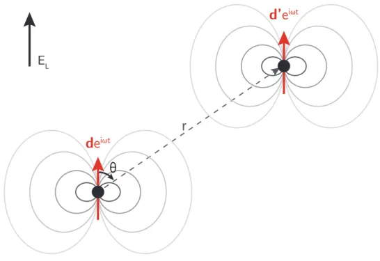
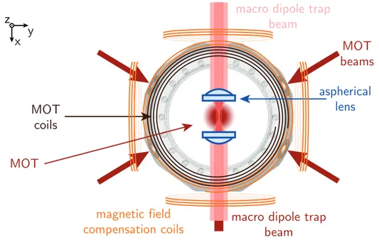
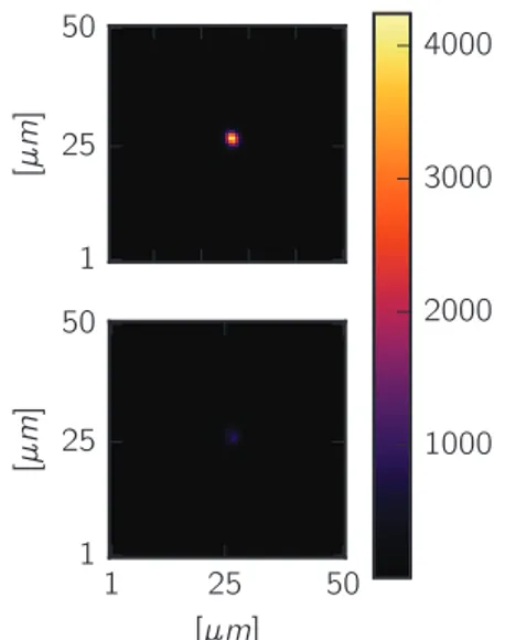
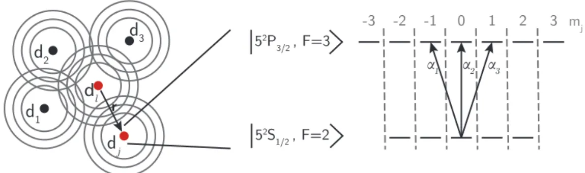
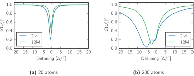
Réponse optique de nuage Rb87 dense
106
0
0
Texte intégral
Figure

+7

Documents relatifs