A local multiple proper generalized decomposition based on the partition of unity

Science Arts & Métiers (SAM)

is an open access repository that collects the work of Arts et Métiers Institute of

Technology researchers and makes it freely available over the web where possible.

This is an author-deposited version published in: https://sam.ensam.eu Handle ID: .http://hdl.handle.net/10985/17949

To cite this version :

Ruben IBAÑEZ, Emmanuelle ABISSET-CHAVANNE, Francisco CHINESTA, Antonio HUERTA, Elías G. CUETO - A local multiple proper generalized decomposition based on the partition of unity International Journal for Numerical Methods in Engineering Vol. 120, n°2, p.139152 -2019

Any correspondence concerning this service should be sent to the repository Administrator : archiveouverte@ensam.eu

A local multiple proper generalized decomposition based on

the partition of unity

Rubén Ibáñez

1

_{Emmanuelle Abisset-Chavanne}

1

_{Francisco Chinesta}

2

Antonio Huerta

3

_{Elías Cueto}

4 1_{ICI - High Performance Computing}

Institute, Ecole Centrale de Nantes, Nantes, France

2_{ESI Group Chair @ PIMM - Procédés et}

Ingénierie en Mécanique et Matériaux, Ensam ParisTech, Paris, France

3_{Laboratori de Calcul Numeric,}

Universitat Politecnica de Catalunya, BarcelonaTech, Barcelona, Spain

4_{Aragon Institute of Engineering}

Research, Universidad de Zaragoza, Zaragoza, Spain

Correspondence

Francisco Chinesta, ESI Group Chair @ PIMM - Procédés et Ingénierie en Mécanique et Matériaux, Ensam ParisTech, 151 boulevard de l'Hôpital, Paris, France.

Email: Francisco.Chinesta@ensam.eu

Funding information

European Union's Horizon 2020 research and innovation; Marie Sklodowska-Curie, Grant/Award Number: 675919; Spanish Ministry of Economy and

Competitiveness, Grant/Award Number: DPI2017-85139-C2-1-R; Regional Government of Aragon; European Social Fund, Grant/Award Number: T24 17R

Summary

It is well known that model order reduction techniques that project the solu-tion of the problem at hand onto a low-dimensional subspace present difficulties when this solution lies on a nonlinear manifold. To overcome these difficulties (notably, an undesirable increase in the number of required modes in the solu-tion), several solutions have been suggested. Among them, we can cite the use of nonlinear dimensionality reduction techniques or, alternatively, the employ of linear local reduced order approaches. These last approaches usually present the difficulty of ensuring continuity between these local models. Here, a new method is presented, which ensures this continuity by resorting to the paradigm of the partition of unity while employing proper generalized decompositions at each local patch.

K E Y WO R D S

local reduced order modeling, model order reduction, partition of unity, proper generalized decomposition

1

I N T RO D U CT I O N

The finite element method (FEM) is the ubiquitous technique for the approximation of partial differential equations (PDEs). Its generality has led it to succeed in many areas of engineering interest. However, when real-time or many-query applications are envisaged, it is well known to be a technique somewhat slow. In recent years, model order reduction (MOR) techniques have shown that a minimum number of carefully-chosen degrees of freedom may be enough for an accurate solution of these same PDE. Instead of choosing general-purpose piecewise polynomials as basis functions, MOR techniques construct ad hoc basis functions following different techniques. For instance, proper orthogonal decom-position (POD)1-5 _{constructs an efficient basis from a set of precomputed snapshots of the full-order PDE solution, ie,}

u(x, t) =

N ∑

i=1

where, very much like in the finite element context,𝛼iare a set of time-dependent coefficients that evolve in time, and

𝜙i(x)are time-independent basis functions obtained by some algebraic treatment of the system snapshots. For instance, many MOR techniques employ the most energetic eigenfunctions of the snapshot autocorrelation matrix to construct these𝜙_i(x). These play a similar role to the finite element (FE) shape functions, albeit they are global instead of local. Other techniques, such as reduced basis methods, for instance,6-8employ some snapshots of the full-order solution as basis for the approximate solution of the system. These snapshots are calculated in a greedy fashion, at time (or parameter) instants at which the error in the approximation is maximal.

It is important to note that Equation (1) constitutes, in fact, a separated expression of the solution (note the space-time separation, which also holds in FE approximations). Assuming this separate or affine decomposition of the solution is also on the origin of another family of MOR techniques coined as proper generalized decomposition (PGD).9-12_These

methods compute the basis function on the fly, that is to say, by means of a greedy algorithm that enriches succes-sively the basis until the desired precision is achieved. This methodology has proven to be very effective for a wide variety of high-dimensional problems ranging from the resolution of Fokker-Planck equation13 _{to patient-specific liver}

responses,14,15_{structural dynamics,}16_{computational rheology,}17_{or, more generally, to any parametric problem that could}

be written in separate form.13

There are situations, however, when the solution is highly nonseparable. In other words, the solution of the problem lives on a nonlinear manifold. In this situation, what MOR techniques do is to project the solution on the tangent space to the manifold at a given (time or parameter) point.18 _{This leads to poor approximation properties far from the}

tan-gency point, unless special techniques are chosen, as in the work of Niroomandi et al,19_{for instance, where asymptotic}

expansions were used.

A way to alleviate this problem is to follow the same philosophy than nonlinear-dimensionality reduction methods. For instance, locally-linear-embedding20tries to unveil the latent variables by means of imposing a local linear variation on the function, which will change from neighborhood to neighborhood. Another technique that deals with nonlinear problems is the so-called kernel principal component analysis.21 In this particular case, the definition of an efficient kernel function allows to project the snapshots to high-dimensional spaces (potentially infinite dimensional) in which the solution manifold is flat. In this particular situation, standard interpolation techniques work well.

Badías et al22_{studied the case of a moving source in a transient heat transfer problem. The problem of the}

nonsepara-bility of the solution was circumvented by means of making a partition of the time domain, dedicating a different PGD for each partition. However, the imposition of the interface conditions will become a tedious task when dealing with partitions involving variables other than time.

The main objective of this paper is to develop a generalized PGD formulation in which continuity between subdomains is guaranteed. This will be achieved by resorting to the partition of unity (PU) paradigm.23,24_{By employing the PU,}

conti-nuity of the solution is guaranteed if the chosen PU is continuous. This will allow us to glue different PGD approximations defined at particular regions of the space, time, or parameter spaces, thus ensuring a global solution with a minimum of degrees of freedom.

The structure of this paper is organized as follows. The second section depicts the general aspects of the proposed methodology; the third section shows the capability of the method to approximate highly nonlinear functions; the fourth section shows applications for different PDEs from fully diffusive to transient equations; and the fifth section will be devoted for the conclusions. All details related to the variational form will be given in the Appendix.

2

BA S I C S O F T H E M ET H O D

The method here proposed is based, as mentioned earlier, in the application of the PU paradigm.23,24In essence, the PU method states that, given a collection of nonoverlapping patches defined over the domain Ω, Ωi, i = 1, … , npatch, a PU𝜑i defined on these patches (ie,∑_i𝜑i=1 everywhere in the domain), and function spaces Vi, associated to each patch, the approximation obtained by V = n_patch ∑ i=1 𝜑iVi

For the sake of simplicity, but without loosing generality, the local PGD method here presented is illustrated by starting with a weak form related to a general two-dimensional PDE, ie,

(u∗_{(x, 𝑦), u(x, 𝑦); 𝛍) = (u}∗_{(x, 𝑦), 𝑓(x, 𝑦)) in Ω.}

Normally, solving the weak form (2) requires an approximation space for the essential variable u(x, y) and its associated variation u∗_{(x, y). The classical FE approximation, ie,}

u(x, 𝑦) =∑

i∈

Ni(x, 𝑦)ui,

where is the entire set of shape functions defined over the integration domain, Ω, satisfies the PU and linear consistency

properties, _∑ i∈ Ni(x, 𝑦) = 1, ∀ x, 𝑦 ∈ Ω, ∑ i∈ Ni(x, 𝑦)xi=x, ∀ x, 𝑦 ∈ Ω, ∑ i∈ Ni(x, 𝑦)𝑦i=𝑦, ∀ x, 𝑦 ∈ Ω.

The main ingredient of the method here proposed is the combination of the FE shape functions, Ni(x, y), as an example of very convenient PU, enriched with low rank PGD approximations. Therefore, each degree of freedom uiassociated to the FEM shape function Ni(x, y) will be enriched with a PGD approximation, aiming to capture the details of the solution, which are not captured by the standard low-order FE meshes. Therefore, the approximation of the solution will read

u(x, 𝑦) =∑ i∈ Ni(x, 𝑦) M ∑ k=1 X_ki(x)Y_ki(𝑦), where Xi k(x)and Y i

k(x)functions are the kth one-dimensional modes related to the ith PGD.

Several approaches can be adopted to define the trial function. In this particular case, a Bubnov-Galerkin projection is selected. Hence, the same approximating space is chosen for u(x, y) and u∗_{(x, y), ie,}

u∗(x, 𝑦) =∑ i∈

Ni(x, 𝑦) (

X_Mi∗(x)Y_Mi(𝑦) + X_Mi (x)Y_Mi∗(𝑦)). (2)

It is worth noting the greedy nature of the PGD algorithm, since the variation only takes into account the last, Mth, PGD mode. Previous modes are considered as known, and therefore do not appear in Equation (2). Furthermore, a nonlinear problem, which has been created due to the separation of variables (note that we solve for a pair of functions, XM, YM), is solved using an alternate direction scheme. Conceptually speaking, it is not necessary to have the same number of modes,

M, for each macroshape function in. A possible strategy would be to stop enriching with new modes in areas where the residual of the equation is low enough. In this first work, all PGDs are enriched with the same number of modes, M, as the main focus is placed on the methodology itself and proving that combining different PGDs within a continuous framework could be useful to obtain separated solutions in complex scenarios where standard PGD performance is decimated. Indeed, the definition of mode adopted herein is the number of separated functions (1 per element in the set) that has to be given to the macropartition to reproduce the solution. In other words, the number of modes is equal to M. It is also important to reckon that the size of the mode will increase according to the number of elements in, since the mode involves as many separated functions per direction as number of degrees of freedom in.

The properties of the method will change depending on the way FE shape functions are defined. Figure 1 exemplifies the partition when piecewise constant shape functions are used. As it can be seen, no overlapping between different PGDs exists. Therefore, extra effort has to be done to set proper interface conditions along the red lines appearing in the same figure. This situation would be equivalent to the method described in the work of Badías et al.22_{This is in sharp}

contrast with the purely additive approach to couple FE and PGD proposed in the work of Ammar et al25or in the work of Quesada et al,26 _{for instance. In that case, the method resembled the s-version of the FEM}27_{or the multiscale FEM}

FIGURE 1 Left, piecewise constant finite element approximation. Center, domain of influence of ith proper generalized decomposition (PGD). Right, domain of influence of kth PGD. As can be noticed, no overlapping exists between different PGD approximations

FIGURE 2 Left, piecewise linear partition of unity. Center, domain of influence of ith proper generalized decomposition (PGD). Right, domain of influence of kth PGD

details of the solution, which usually provoke an increase in the number of PGD modes. Here, on the contrary, we develop an approximation by means of multiple PGD approximations, glued together by means of the PU paradigm. We have coined this method as PU-PGD.

Figure 2 depicts a piecewise linear partition of the domain. As it can be noticed, a quadrilateral element has contri-butions coming from four different PGDs. The coupling conditions between different PGDs are automatically taken into account in the elemental contributions. Indeed, this kind of partition imposes a smooth transition between PGDs, which vary continuously along the domain in accordance with the partition of the domain.

It is worth mentioning that the full potential of PGD approximation resides in the capability of writing the integral form in a separated manner. By doing that, all integrals in a high-dimensional space will be split into a product of integrals related to each one of the subspaces. For the sake of simplicity, we will assume that the shape functions Ni(x, y) are exactly separable in one single mode

Ni(x, 𝑦) = N_ix(x)N_i𝑦(𝑦).

It is important to notice that this will be the case, for instance, of 2D quadrilateral elements with straight and parallel sides. Even though this assumption may be seen as a limitation, it is important to notice that there are some variables, such as time or parameters, that naturally admit cartesian decompositions. Therefore, when dealing with a complex spatial geometry that evolves in time, a smart partition would be to keep the space variable as is. Nevertheless, this very first work is meant to provide an insight of the method, thus, all results presented in the sequel will be related to piecewise linear FE shape functions based on squared elements.

3

PU

- P G D FO R A P P ROX I M AT I O N P RO B L E M S

3.1

Basics of the method

In this section, we analyze the capability of the proposed methodology in approximation problems of the form

∫

Ω

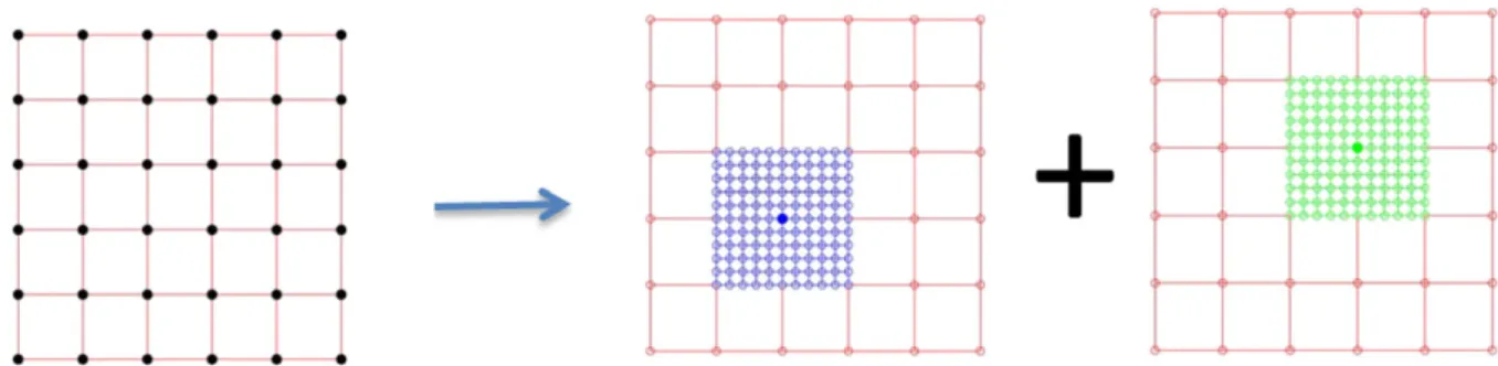
FIGURE 3 In the case of bilinear finite elements, there is one proper generalized decomposition (PGD) enrichment per node [Colour figure can be viewed at wileyonlinelibrary.com]

where a function f(x, y) is to be approximated in an PU-PGD framework. As it can be noticed, there are no partial deriva-tives involved in this type of problems. Instead, just a compact expression of the function f(x, y) is sought. It is important to highlight that continuity is not a requirement, given the fact that no differential equation is involved in this particu-lar case. Indeed, considering a discontinuous approximation space with a much more local procedure will provide better results if the function to be captured presents high gradients or even discontinuities. However, this very first example is included as an initial point to illustrate the continuous approach, which is mandatory to solve PDEs.

Following the spirit of standard FE approximation, the integral over the entire domain Ω is split into a sum of integrals for each one of the FEs Ωeappearing in the domain. Recall that piecewise bilinear shape functions present contributions from four different PGDs per element (one for each corner), as shown in Figure 3.

It is important to notice that the ith PGD, thanks to the PU, affects the support of each FE node, and thus four elements in a regular lattice.

Omitting the dependence with respect to space variables, x and y, and thanks to the separability of the FE shape function (if defined in a regular lattice as a tensorial product of one-dimensional functions), the first term in the integral form of Equation (3) particularized for a element Ωereads

∫ Ωe u∗_{udxd𝑦 =} 4 ∑ i=1 4 ∑ 𝑗=1∫_Ω e N_ixN_i𝑦(X_Mi Y_Mi )∗ ( N_𝑗xN_𝑗𝑦 M ∑ k=1 X𝑗 kY 𝑗 k ) dxd𝑦.

The next step is to split the 2D integral form into a tensorial product of 1D integrals as

∫ Ωe u∗udxd𝑦 = 4 ∑ i=1 4 ∑ 𝑗=1 M ∑ k=1∫_x X_Mi∗N_ixN_𝑗xX_k𝑗_{dx ∫} 𝑦 Y_Mi N_i𝑦N_𝑗𝑦Y_k𝑗d𝑦 + 4 ∑ i=1 4 ∑ 𝑗=1 M ∑ k=1∫_x X_Mi N_ixN_𝑗xX_k𝑗_{dx ∫} 𝑦 Y_Mi∗N_i𝑦N_𝑗𝑦Y_k𝑗d𝑦. (4)

As can be noticed, the variation along the x direction shares all the operators with the variation along the y direction. Indeed, this property arises naturally from the alternate directions scheme that is used to solve the nonlinear system of the PGD.

With the source term f(x, y) expressed in a separated format (eg, by invoking the SVD) as

𝑓(x, 𝑦) = Z ∑ z=1 𝑓x z(x)𝑓z𝑦(𝑦),

the right-hand side term appearing in Equation (3) reads

∫ Ωe u∗𝑓dxd𝑦 = 4 ∑ i=1 Z ∑ z=1∫ x X_Mi∗N_ix𝑓zxdx ∫ 𝑦 Y_MiN_i𝑦𝑓_z𝑦d𝑦 + 4 ∑ i=1 Z ∑ z=1∫ x X_Mi N_ix𝑓zxdx ∫ 𝑦 Y_Mi∗N_i𝑦𝑓_z𝑦d𝑦,

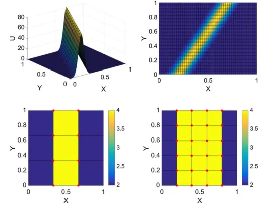
FIGURE 4 Left, 3D view of f₁(x, y). Right, top view of f₁(x, y) [Colour figure can be viewed at wileyonlinelibrary.com]

FIGURE 5 Left, domain enriched with 8 proper generalized decompositions (PGDs). Right, domain enriched with 24 PGDs. Red points, centroid of each PGD. The legend shows the number of PGD enrichments affecting each element

3.2

A preliminar example

Let us illustrate the methodology by analyzing a highly nonseparable function

𝑓1(x, 𝑦) = 10

𝜎√2𝜋

e−(x−(v2𝑦+x0))2𝜎2 ,

where𝜎 = 0.05, v = 0.5, and x0=0.2.

Figure 4 depicts the resulting u(x, y) = f₁(x, y) scalar field from different perspectives. As it can be seen, the source term is going through the diagonal of the domain, generating a highly nonseparable function. Indeed, a standard PGD algorithm encounters many problems to capture such kind of solution.

Two different partitions of the domain have been tested, as shown in Figure 5. Along the right and left sides of the domain, no enrichment is added to the FE approximation since the sought solution is already zero along this boundary. It is important to reckon that right and left sides of the domain could have been enriched, since no boundary conditions need to be imposed in this approximation problem. However, the fact that compatible boundary conditions (ie, zero along the right and left sides) can be imposed was used as a validation point for the next numerical examples involving PDEs. The elements are colored in accordance with the number of active PGDs acting in each element.

Figure 6 shows the reconstructed solution using 4 modes per local PGD, when the domain has 8 active PGDs (left) and 24 PGDs (right). As it can be seen, even though both approximations capture the main features of the solution, the solution using 24 PGDs is slightly better than the one with 8 PGDs.

FIGURE 6 Left, solution with 8 proper generalized decomposition (PGDs). Right, solution with 24 PGDs. Every PGD enrichment incorporates four modes [Colour figure can be viewed at wileyonlinelibrary.com]

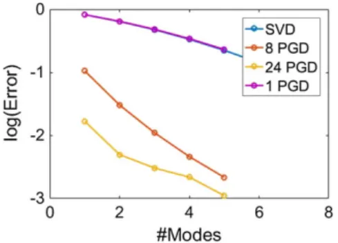
FIGURE 7 Convergence error for the approximation problem. Comparison between singular value decomposition (SVD), standard proper generalized decomposition (PGD), and two different local strategies

Figure 7 shows the convergence error for the approximation of f₁(x, y). The relative error is measured as

m₌ ‖‖ure𝑓−u m‖‖ ‖‖ure𝑓‖‖ , where um_{is the reconstructed solution using m modes. u}

ref represents the ground truth. As can be noticed, singular

value decomposition (SVD) method suffers from separating this kind of solutions, having a slow decay of the relative error with respect to the number of modes. As it is well known from the literature, standard PGD in two dimensions is exactly equivalent to SVD when an identity operator is employed (the so-called PGD in approximation29,30_{). On the other}

hand, using the PU-PGD algorithm, the relative error decays much faster than the one related to standard SVD or PGD approximations.

It is important to notice that the more a domain is partitioned, the smaller the relative error is. This behavior is expected since the smaller the elements are, the easier it is to capture a local behavior. However, the price to pay is that the cost of computing one mode per PGD will increase just like the storage cost as well. Certainly, systems solved in the fixed point iteration are not local due to the fact that macroshape functions are overlapped. If the macropartition involves # shape functions and each local PGD is discretized using nxand nydegrees of freedom, the number of unknowns in each PGD fixed point are # · nxand # · n𝑦for x and y directions, respectively. Therefore, it is important to keep in mind that refining the macromesh would reduce the number of modes M to represent the solution, but it would also increase the computational cost for obtaining one mode. However, the main focus of this work was to prove that the proposed methodology was able to obtain separated solutions in scenarios where standard PGD performance was not good enough.

4

PU

- P G D FO R T H E S O LU T I O N O F PA RT I A L D I F F E R E N T I A L EQ UAT I O N S

The aim of this section is to show the potential of the proposed methodology when applied to the solution of different PDEs. We consider examples of increasing complexity. Therefore, the first test case is a pure diffusion equation. The second case is a convection-reaction-diffusion equation. Finally, the last example relates to a transient thermal problem with a moving source term. Even though the construction of the operators for each PDE follows the same trend than the ones presented in the PU-PGD in approximation, further details are given in the appendix.

4.1

Diffusion PDE

We first consider the following weak form corresponding to a diffusion problem:

∫ Ω 𝜂∇u∗_{· ∇udxd} 𝑦 = ∫ Ω u∗_𝑓 1dxd𝑦.

Vanishing Dirichlet boundary conditions are imposed on the entire boundary. The source term is equal to the function

FIGURE 8 Left, 3D view of u(x, y). Right, planar view of u(x, y) for the diffusion equation [Colour figure can be viewed at wileyonlinelibrary.com]

FIGURE 9 Left, problem solved with four proper generalized decomposition (PGDs). Right, problem solved with 16 PGDs. Red points represent finite element nodes enriched with PGD. The legend represents the number of PGDs per element

Figure 8 depicts the reference u(x, y) scalar field for the diffusion equation from different perspectives. It has been obtained with a 80 × 80 FE discretization. As it can be seen, the solution diffuses the source term through the diagonal of the domain.

Two different PGD enrichments have been tested, as shown in Figure 9. The PGD enrichments acting on top, bottom, left, and right sides are set to zero to be consistent with the problem statement, where zero Dirichlet boundary conditions are imposed along the entire boundary domain. The red points indicate the enriched nodal supports. The elements are colored in accordance with the number of enriching PGDs. Elements on the corners have only one active PGD, whereas elements on the sides have two active PGDs and interior elements have four active PGDs.

The reconstructed solution using four modes per PGD enrichment, when the domain has four active PGDs (left) and sixteen PGDs (right), is in perfect visual agreement with the reference solution appearing in Figure 9.

Figure 10 shows the convergence error for the diffusive equation. As it can be noticed, all methods converge monoton-ically, SVD being the one that presents the slower convergence with respect the number of modes. Standard PGD shows a similar convergence rate to SVD, as expected. Even if no formal proof exists of this behavior for operators other than the identity, this is the observed rate for all the experiments considered so far. Finally, using the multi-PGD algorithm presents a faster decay in the relative error.

FIGURE 10 Convergence error for the diffusion problem. Comparison between the number of modes provided by singular value decomposition (SVD), standard proper generalized decomposition (PGD), and two different enrichment strategies considered so far

FIGURE 11 Left, 3D view of the reference solution u(x, y). Right, planar view of u(x, y) for convection-reaction-diffusion equation [Colour figure can be viewed at wileyonlinelibrary.com]

4.2

Convection-reaction-diffusion PDE

In this subsection a convection-reaction-diffusion equation is studied. Indeed, the major novelty is the introduction of the convective term since it will involve a nonsymmetric operator. The weak form related to the this equation is

∫

Ω

u∗_{v · ∇u +𝜂∇u}∗_{· ∇u +𝜎u}∗_{u dxd}

𝑦 = ∫

Ω

u∗_𝑓

2dxd𝑦, (5)

where vanishing Dirichlet boundary conditions are considered on the entire boundary. The integration domain is Ω =

[0, 1] × [0, 1]. The convective velocity field is assumed to be v = 500(y − 0.5, 0.5 − x)T_{. The reaction term is set to𝜎 = 10}

and the diffusion coefficient to𝜂 = 1. Regarding the source term, a Gaussian located in [x0, y0] = [0.75, 0.75] as

𝑓2(x, 𝑦) = √800

2𝜋

e−(x−x0)02 +(𝑦−𝑦0)2.005

is considered.

Figure 11 depicts the reference u(x, y) scalar field for the solution of Equation (5) (computed by employing an 80×80 FE mesh, thus with no need for stabilization) from different perspectives. Note how the Gaussian source term is convected circularly according to the prescribed velocity field. Moreover, the diffusion term makes the Gaussian to be smoothed along its convection path.

The same partitions than in the diffusive case have been tested, as shown in Figure 9, since also vanishing Dirichlet boundary conditions are imposed along the entire boundary of the domain. Figure 12 shows the reconstructed solution using 4 modes per local PGD, when the problem has been approximated by 4 PGDs (left) and 16 PGDs (right). Notice how the approximation related to 4 PGDs does not capture the solution well. Indeed, a higher number of modes will be needed to converge to the reference solution. On the other hand, the solution involving 16 PGDs is in perfect accordance with the reference solution, capturing all the features of the scalar field without any perceptible oscillation.

Figure 13 shows the convergence of the relative error in logarithmic scale for the SVD and the two different partitions proposed for the CDR equation. It can be clearly seen that the convergence related to the 4 PGD partition is the slowest one. Indeed, this problem is derived from the fact that the first PGD modes have to capture a highly nonlinear behavior, meaning that this partition will require a high amount of modes to converge to the real solution. On the other hand, the 16 PGD partition convergence is quite fast compared with the other two methods.

FIGURE 12 Solution of the convection-diffusion-reaction equation. Left, 4 proper generalized decomposition (PGDs). Right, 16 PGDs. Both solutions have four modes per PGD [Colour figure can be viewed at wileyonlinelibrary.com]

FIGURE 13 Convergence plot for the convection-diffusion-reaction problem. Comparison between singular value decomposition (SVD), standard proper generalized decomposition (PGD), and two different enrichment strategies

FIGURE 14 Left, 3D view of u(x, t). Right, top view of u(x, t) for the transient heat transfer equation [Colour figure can be viewed at wileyonlinelibrary.com]

4.3

Transient heat transfer equation

This last example is devoted to the analysis of a transient 1D heat transfer problem, a test proposed by Idelsohn31_{to verify}

the compactness of different MOR techniques, ie,

∫ Ω u∗𝜕u 𝜕t +𝜂 𝜕 u∗ 𝜕x 𝜕u∗ 𝜕x dx dt = ∫ Ω u∗𝑓3dx dt,

where the diffusion coefficient is set to𝜂 = 0.01.

The domain of study is Ω = Ωx× Ωt = [0, 1] × [0, 1]. The set of boundary conditions imposed for the field u(x, t) is

u(x, 0) = 0, u(0, t) = 0, and u(1, t) = 0. The source term f3(x, y) is

𝑓3(x, t) = 10 𝜎√2𝜋 e−(x−(vt+x0)) 2 2𝜎2 , where𝜎 = 0.05, v = 0.5, and x0=0.1.

Figure 14 depicts the reference u(x, y) scalar field for the transient heat equation from different perspectives. Again, an 80 × 80 FE mesh of bilinear elements has been employed. This kind of PDE creates a boundary layer along the diagonal of the space-time domain, which is very hard to capture when using standard separate approximations like POD and classical PGD.

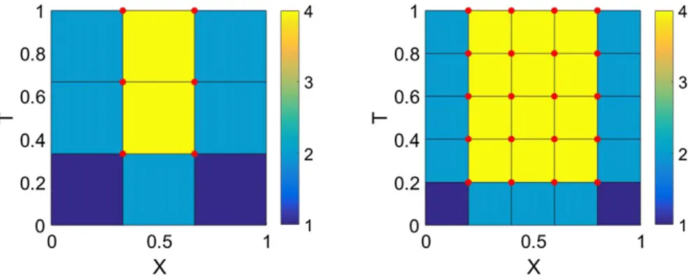
FIGURE 15 Left, problem solved with 6 proper generalized decompositions (PGDs). Right, problem solved with 20 PGDs. Red points represent the finite element nodes that incorporate an enrichment. The legend indicates the number of PGDs per element

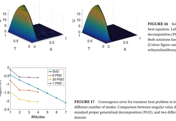
FIGURE 16 Solution of the transient heat equation. Left, 6 proper generalized decomposition (PGDs). Right, 20 PGDs. Both solutions have four modes per PGD [Colour figure can be viewed at

wileyonlinelibrary.com]

FIGURE 17 Convergence error for transient heat problem in logarithmic scale for different number of modes. Comparison between singular value decomposition (SVD), standard proper generalized decomposition (PGD), and two different partitions of the domain

Two different enrichment strategies have been tested, as shown in Figure 15. It is important to highlight that PGDs acting on x = 0, x = 1, and t = 0 are set to zero to satisfy the null Dirichlet and initial boundary conditions in this portion of the boundary. However, the PGD acting on the interior nodes of the line t = 1 is not set to zero. This fact is a direct consequence of the pure convective behavior associated to the time variable. Indeed, the line t = 1 acts like an outflow boundary, thus, no condition should be imposed there to ensure the well-possedness of the problem.

Figure 16 shows the reconstructed solution using four modes per local PGD, when the domain has 6 active PGDs (left) and 20 PGDs (right). Notice how both approximations capture the main features of the reference solution. However, the approximation with 6 active PGDs presents small oscillations due to the lack of PGD modes to converge to the reference solution.

Figure 17 shows the convergence plot for the SVD and the two different enrichments proposed for the transient heat equation. It can be stated that both partitions present a faster convergence than the SVD convergence. However, the convergence slope of the PGD partitions tend to be flatter than the SVD one in the last part of the convergence plot.

To establish a fair comparison between the methods presented so far, it is interesting to perform a comparison on a per-degree-of-freedom basis. Figure 18 shows the convergence plot related to the transient thermal problem in which the standard PGD approximation has the same degrees of freedom than the PU-PGD approximation. It is worth noting the fast convergence of the PU-PGD, which comes from the fact that it takes advantage of the locality of the solution, avoiding problem of highly nonlinear global functions.

FIGURE 18 Convergence plot for Idelsohn problem using different partitions of the domain. All approximations have the same number of degrees of freedom. PGD, proper generalized decomposition; SVD, singular value decomposition

5

D I S C U S S I O N. F U T U R E WO R K

The method presented overcomes some of the most important limitations of standard PGD approximations. These, which are indeed common to every MOR technique, are related to the nonlinearity of the solution map. As in previous works, in the literature, an appealing strategy is to develop local approximations. This approach comes from the well-known fact that a manifold is flat in the neighborhood of every point.

The local multiple approximations here developed have shown to reconstruct the solution up to a certain tolerance by using a moderate number of modes. However, as previously stated, the size of the mode will increase according to the macropartition of the domain. Therefore, the choice of the macropartition constitutes one of the central key points of this approach. A macropartition that minimizes the number of macroelements while it reduces the number of modes to represent the solution would be the optimal one. Certainly, a possible future route is to mimic the element refinement in FEM, starting with a coarse macropartition and perform only macrorefinement in areas where the residual of the equation is high enough.

One drawback, however, of the proposed technique is related to the curse of dimensionality in high-dimensional prob-lems. The PU-PGD approach introduces a mesh to construct the PU. This may result in prohibitive computational costs if the number of dimensions of the solution grows.

However, as in previous local approaches of PGD,22_{there is no need to partition every dimension into elements. Instead,}

only those parameter interval of interest that cause the most nonlinear response of the solution should be partitioned. Knowing in advance the nonlinear shape of the solution manifold is by no means straightforward. This constitutes our current effort of research.

AC K N OW L E D G E M E N T S

This project has received funding from the European Union's Horizon 2020 research and innovation program under the Marie Sklodowska-Curie grant agreement 675919. Moreover, by the Spanish Ministry of Economy and Competitiveness through Grant DPI2017-85139-C2-1-R and by the Regional Government of Aragon and the European Social Fund research group T24 17R.

O RC I D

Elías Cueto https://orcid.org/0000-0003-1017-4381

R E F E R E N C E S

1. Karhunen K. Uber lineare methoden in der wahrscheinlichkeitsrechnung. Ann Acad Sci Fennicae ser Al Math Phys. 1946;37(1). 2. Lo ˙eve MM. Probability Theory. The University Series in Higher Mathematics. 3rd ed. Princeton, NJ: Van Nostrand; 1963.

3. Park HM, Cho DH. The use of the Karhunen-Lo ˙eve decomposition for the modeling of distributed parameter systems. Chem Eng Sci. 1996;51(1):81-98.

4. Meyer M, Matthies HG. Efficient model reduction in non-linear dynamics using the Karhunen-Lo ˙eve expansion and dual-weighted-residual methods. Comput Mech. 2003;31(1-2):179-191.

5. Chinesta F, Ladevèze P. Separated Representations and PGD-based Model Reduction. Udine, Italy: CISM; 2014.

6. Rozza G, Huynh DBP, Patera AT. Reduced basis approximation and a posteriori error estimation for affinely parametrized elliptic coercive partial differential equations. Computat Methods Eng. 2008;15:229. https://doi.org/10.1007/s11831-008-9019-9

7. Quarteroni A, Rozza G, Manzoni A. Certified reduced basis approximation for parametrized PDE and applications. J Math Ind. 2011;1(1):3. 8. Rozza G. Fundamentals of reduced basis method for problems governed by parametrized PDEs and applications. In: Ladeveze P, Chinesta F, eds. Separated Representation and PGD Based Model Reduction: Fundamentals and Applications. Vienna, Austria: Springer; 2014.

9. Ammar A, Mokdad B, Chinesta F, Keunings R. Anew family of solvers for some classes of multidimensional partial differential equations encountered in kinetic theory modeling of complex fluids. J Non-Newton Fluid Mech. 2006;139:153-176.

10. Chinesta F, Ammar A, Cueto E. Recent advances in the use of the proper generalized decomposition for solving multidimensional models. Arch Comput Methods Eng. 2010;17(4):327-350.

11. Ladevèze P, Passieux J-C, Néron D. The latin multiscale computational method and the proper generalized decomposition. Comput Methods Appl Mech Eng. 2010;199(21-22):1287-1296.

12. Chinesta F, Cueto E. PGD-Based Modeling of Materials, Structures and Processes. Cham, Switzerland: Springer International Publishing; 2014.

13. Pruliere E, Chinesta F, Ammar A. On the deterministic solution of multidimensional parametric models using the proper generalized decomposition. Math Comput Simul. 2010;81(4):791-810.

14. Mena A, Bel D, Alfaro I, González D, Cueto E, Chinesta F. Towards a pancreatic surgery simulator based on model order reduction. Adv Model Simul Eng Sci. 2015;2(1):31.

15. González D, Cueto E, Chinesta F. Computational patient avatars for surgery planning. Ann Biomed Eng. 2015;44(1):35-45.

16. González D, Cueto E, Chinesta F. Real-time direct integration of reduced solid dynamics equations. Int J Numer Methods Eng. 2014;99(9):633-653.

17. Chinesta F, Ammar A, Leygue A, Keunings R. An overview of the proper generalized decomposition with applications in computational rheology. J Non-Newton Fluid Mech. 2011;166(11):578-592.

18. Amsallem D, Farhat C. An interpolation method for adapting reduced-order models and application to aeroelasticity. AIAA Journal. 2008;46:1803-1813.

19. Niroomandi S, Alfaro I, Cueto E, Chinesta F. Model order reduction for hyperelastic materials. Int J Numer Methods Eng. 2010;81(9):1180-1206.

20. Roweis ST, Saul LK. Nonlinear dimensionality reduction by locally linear embedding. Science. 2000;290(5500):2323-2326.

21. Schölkopf B, Smola A, Müller KR. Kernel principal component analysis. Advances in Kernel Methods - Support Vector Learning. Cambridge, MA: MIT Press; 1999:327-352.

22. Badías A, González D, Alfaro I, Chinesta F, Cueto E. Local proper generalized decomposition. Int J Numer Methods Eng. 2017;112(12):1715-1732.

23. Babuška I, Melenk JM. The partition of unity finite element method: basic theory and applications. Comput Meth Appl Mech Eng. 1996;139:289-314.

24. Babuška I, Melenk JM. The partition of Unity Method. Int J Numer Methods Eng. 1997;40:727-758.

25. Ammar A, Chinesta F, Cueto E. Coupling finite elements and proper generalized decompositions. Int J Multiscale Comput Eng. 2011;9(1):17-33.

26. Quesada C, González D, Alfaro I, Cueto E, Chinesta F. Computational vademecums for real-time simulation of surgical cutting in haptic environments. Int J Numer Methods Eng. 2016;108(10):1230-1247.

27. Fish J. The s-version of the finite-element method. Comput Struct. 1992;43(3):539-547.

28. Rank E, Krause R. A multiscale finite-element method. Comput Struct. 1997;64(1-4):139-144. Computational Structures Technology. 29. Chinesta F, Keunings R, Leygue A. The Proper Generalized Decomposition for Advanced Numerical Simulations. Cham, Switzerland:

Springer International Publishing; 2014.

30. Le Bris C, Leli ˙evre T, Maday Y. Results and questions on a nonlinear approximation approach for solving high-dimensional partial differential equations. Constructive Approximation. 2009;30(3):621.

31. Neron D, Ladeveze P. Idelsohns benchmark. 2013.

A P P E N D I X

E L E M E N TA L O P E R ATO R S

In this appendix, we give exhaustive details about the construction of the operators required to make the PU-PGD approx-imation for the different PDEs studied in this paper. Detailed information was given for the case of the PU-PGD in approximation. Hence, further details will be shown related to the diffusive and convective terms.

A.1

Diffusive operator

In this section, a diffusion of a scalar field u(x, y) along the x direction is developed. The derivation for the diffusion along the y direction follows similar guidelines. For the sake of simplicity, but without loosing generality, we will also assume

∫ Ωe 𝜕u∗ 𝜕x 𝜕u𝜕xdxd𝑦 = 4 ∑ i=1 4 ∑ 𝑗=1 M ∑ k=1∫ Ωe ( 𝜕Ni 𝜕x XMi∗YMi +Ni 𝜕Xi∗ M 𝜕x YMi ) ( 𝜕N𝑗 𝜕x Xk𝑗Y 𝑗 k +N𝑗 𝜕X_k𝑗 𝜕x Yk𝑗 ) dxd𝑦 = = 4 ∑ i=1 4 ∑ 𝑗=1 M ∑ k=1∫_x X_Mi∗𝜕N x i 𝜕x 𝜕Nx 𝑗 𝜕x Xk𝑗dx ∫ 𝑦 Y_Mi N_i𝑦N_𝑗𝑦Y_k𝑗d𝑦+ + 4 ∑ i=1 4 ∑ 𝑗=1 M ∑ k=1∫ x 𝜕Xi∗ M 𝜕x Nix 𝜕Nx 𝑗 𝜕x Xk𝑗dx ∫ 𝑦 Y_Mi N_i𝑦N_𝑗𝑦Y𝑗 kd𝑦+ + 4 ∑ i=1 4 ∑ 𝑗=1 M ∑ k=1∫_x 𝜕Xi∗ M 𝜕x NixN x 𝑗 𝜕X_k𝑗 𝜕x dx ∫ 𝑦 Yi MNi𝑦N 𝑦 𝑗Yk𝑗d𝑦+ + 4 ∑ i=1 4 ∑ 𝑗=1 M ∑ k=1∫_x X_Mi∗𝜕N x i 𝜕x N𝑗x 𝜕X_k𝑗 𝜕x dx ∫ 𝑦 Y_Mi N_i𝑦N_𝑗𝑦Y_k𝑗d𝑦. (A1)

It can be highlighted that four different contributions are appearing due to the application of the chain rule. Furthermore, all terms appearing in the last part of Equation (A1) present already a separated format.

A.2

Convective operator

In this section, a pure convection of a scalar field u(x, y) along the x direction is derived. It is important to notice that this case is a particular case of a general convection given by the velocity field v, where a separated representation of the velocity field would be required. The derivation for the convection along the y direction follows similar guidelines. For the sake of simplicity, but without loosing generality, we will also assume that a new mode in the x direction is desired. Therefore, all variations related to the y direction are set to zero, ie,

∫ Ωe u∗𝜕u 𝜕xdxd𝑦 = 4 ∑ i=1 4 ∑ 𝑗=1 M ∑ k=1∫ Ωe NiX_Mi∗Y_Mi ( 𝜕N𝑗 𝜕x Xk𝑗Y 𝑗 k+N𝑗 𝜕X_k𝑗 𝜕x Yk𝑗 ) dxd𝑦 = = 4 ∑ i=1 4 ∑ 𝑗=1 M ∑ k=1∫ x Xi∗ MNix 𝜕Nx 𝑗 𝜕x Xk𝑗dx ∫ 𝑦 Yi MNi𝑦N 𝑦 𝑗Yk𝑗d𝑦+ + 4 ∑ i=1 4 ∑ 𝑗=1 M ∑ k=1∫_x X_Mi∗N_ixN_𝑗x𝜕X 𝑗 k 𝜕x dx ∫ 𝑦 Y_Mi N_i𝑦N_𝑗𝑦Y_k𝑗d𝑦. (A2)

Once again all integrals appearing in the last part of Equation (A2) are written already in a separated way, improving the efficiency of the algorithm.