Interactions océan-atmosphère au sein des cyclones tropicaux du pacifique sud : processus et climatologie

THÈSE

THÈSE

En vue de l’obtention du

DOCTORAT DE L’UNIVERSITÉ DE TOULOUSE

Délivré par : l’Université Toulouse 3 Paul Sabatier (UT3 Paul Sabatier)

Présentée et soutenue le 28/11/2013 par :

Swen JULLIEN

Interactions océan-atmosphère au sein des cyclones tropicaux du Pacifique Sud : processus et climatologie

JURY

Franck ROUX Professeur d’Université Président du Jury Pascale BRACONNOT Directrice de Recherche Rapporteur Bernard BARNIER Directeur de Recherche Rapporteur Fabrice CHAUVIN Ingénieur Météo-France Examinateur Patrick MARCHESIELLO Directeur de Recherche Directeur de thèse Christophe MENKES Chargé de Recherche Co-directeur de thèse Nicholas HALL Professeur d’Université Invité

École doctorale et spécialité :

SDU2E : Dynamique de l’océan et de l’atmosphère Unité de Recherche :

Laboratoire d’Etudes en Géophysique et Océanographie Spatiale (UMR 5566) Directeur(s) de Thèse :

Patrick MARCHESIELLO et Christophe MENKES Rapporteurs :

Ocean response and feedback to

tropical cyclones in the South

Pacific: processes and climatology

Swen Jullien

Remerciements

Mes remerciements vont tout d’abord à Patrick et Christophe qui m’ont permis de réaliser cette thèse avec un encadrement scientifique et humain exceptionnel. Je mesure toute la valeur d’avoir eu des directeurs disponibles, impliqués et com-pétents sur mon sujet, mais également amicaux et qui ont accepté mon caractère quelque peu têtu et franc parfois. . . Je te remercie aussi Patrick, avec le recul, pour l’auto-apprentissage que tu m’as forcé à faire au début (même si ça me faisait parfois râler) et tes réponses que je garderai en mémoire : "t’as cherché sur google?". Je suis finalement devenue une vraie "n3rd" comme disent tes filles. Bien sûr je n’oublierai pas non plus les discussions cinématographiques entre frenchies de la conférence à Kos. Christophe, merci de m’avoir donné le goût de la modélisation, parce que finalement ça me plaît bien, et des discussions scientifiques au café sur le CYGP ou le changement climatique mais aussi de m’avoir permis de partir en campagne en mer entre mon stage et ma thèse. Et puis surtout, après mes séjours à Nouméa, je ne peux que me remémorer avec nostalgie les pique-niques à l’île aux canards et les cafés philosophiques dans le patio avec Andres et les filles. J’en profite donc pour un remerciement aux copines de Calédo Laury, Christelle, Mag, Marion, Steph et JB (désolée tu es passé chez les copines). Merci aussi à Flog de m’avoir donné les contacts nouméens et surtout celui d’un chercheur aux drôles de cheveux bouclés qui fume la pipe.

Un énorme merci à Jérôme pour son aide sans faille sur tout type de fichier log même à 10h de décalage horaire et 17 288 km de distance, et pour son calme impressionnant face à un ordinateur. Sans parler de ses prouesses en planche à voile et des miennes. . .

Je tiens aussi à remercier toute l’équipe cyclone pour son soutien scientifique et particulièrement Nico pour ses programmes shell/fortran et sa liqueur de papaye, Matthieu pour la "cellule psychologique" et son rire, Guillaume pour avoir partager les fameuses discussions WRF avec moi, Ariane pour sa motivation, son enthousiasme et pour la mission Indomix, Margot pour les discussions SPCZ, changement climatique et les dessins de Christophe.

Je remercie également les membres de mon jury de thèse pour leur temps accordé à la lecture de mon manuscrit (en anglais. . . ) et à la soutenance. Un remerciement spécial pour Nick, qui m’a suivi tout au long de mon parcours en météo et océanographie à la fac puis au labo et surtout qui a crée CHEVRE pour qu’on puisse enfin faire des réunions scientifiques et pas administratives !

Un remerciement particulier à toute l’équipe de gestion du LEGOS, Martine, Nadine, Brigitte et Agathe, pour leur aide précieuse pour les missions, leur soutien et leur convivialité. Le LEGOS a de la chance d’avoir des perles comme elles !

Pour mes débuts dans le monde de la recherche et de l’océanographie de terrain avec les missions à la lagune de Lapalme et pour des parties de baby mémorables sur le Marion Dufresne, merci à Pieter et Marc. Sans oublier François qui est le témoin de notre victoire et qui a des supers poissons dans son bureau.

Enfin, tout ce début de chemin parcouru dans les couloirs du LEGOS et sur le terrain aurait vraiment manqué de potins et de discussions de filles sans Marie et Sabine et je suis vraiment contente d’avoir partagé ce temps avec elles.

de rouge d’ailleurs Robin !) et de la pétanque.

Bien sûr cette thèse n’aurait pas été aussi agréable sans la compagnie et le soutien de Yves et Clément qui ont supporté mes questions geek et mes vocif-érations informatiques et avec qui j’ai pu partager des cafés, des croissants, des mojitos/parties de belote et encore bien des choses. Yves, merci aussi d’avoir écouté ma présentation de soutenance quelque chose comme au moins 5 fois ! Je pense que tu aurais finalement pu la faire à ma place.

Pour terminer, plus que des remerciements pour Marc qui a partagé mes moments de motivation qui impliquaient de discuter de pondération de moyenne le soir, comme mes moments de stress (et ceux qui me connaissent savent que je ne suis pas de la plus grande douceur dans ces moments. . . ). Merci aussi de m’avoir laissé partir en Nouvelle-Calédonie et surtout de m’avoir toujours soutenue et de le faire encore.

Contents

Introduction générale

1

Chapter 1 Introduction

3

1.1 Generalities on tropical cyclones

. . . 4

1.1.1 Observations . . . 4

1.1.2 General characteristics . . . 6

1.1.3 The South Pacific . . . 7

1.2 TC formation and intensification

. . . 8

1.3 Ocean response to TCs

. . . 12

1.3.1 Cold wake formation . . . 12

1.3.2 Mixing and upwelling mechanisms. . . 12

1.3.3 The role of ocean structure and dynamics . . . 14

1.3.4 Impact on the ocean climate . . . 15

1.4 Ocean feedback to tropical cyclones

. . . 16

1.5 State of the art modeling of tropical cyclones

. . . 18

1.5.1 Climate models . . . 20

1.5.2 Simple coupled models . . . 20

1.5.3 Realistic coupled models . . . 21

1.5.4 Long-term regional simulations . . . 21

1.6 Manuscript outline

. . . 22

Chapter 2 Development of a coupled model for the

South Pacific

25

2.1 Models

. . . 26

2.1.1 Atmospheric model: WRF . . . 26

2.1.2 Ocean model: ROMS . . . 29

2.1.3 Coupler . . . 31

2.1.3.1 Coupling methodology . . . 31

2.1.3.2 Computational performances . . . 34

2.1.3.3 Note on OASIS coupler . . . 35

2.2 Sensitivity tests

. . . 35

2.2.2 Planetary boundary layer (PBL) . . . 37

2.2.3 Cloud microphysics . . . 38

2.2.4 Shortwave radiation . . . 38

2.2.5 Surface drag . . . 39

2.2.6 Skin SST . . . 41

2.2.7 Land surface model . . . 42

2.2.8 Sponge layers . . . 43

2.2.9 Sensitivity to vertical resolution . . . 43

2.3 Methodology

. . . 43

2.3.1 TC tracking and SPEArTC database . . . 43

2.3.2 Forced model: cold track filtering technique . . . 47

2.3.3 Statistics and error bars . . . 49

2.3.3.1 Interannual variability . . . 49

2.3.3.2 Seasonal or intensity variability . . . 51

2.3.3.3 Similarity of forced and coupled models distributions . 52 2.3.4 Compositing methodology . . . 53

2.4 Summary of the experiments

. . . 54

Chapter 3 Climatology of the South Pacific and

model validation

57

3.1 Validation datasets

. . . 58

3.1.1 Ocean properties . . . 58

Pathfinder SST . . . 58

CARS climatology . . . 58

Montegut et al. [2004] MLD climatology . . . 58

3.1.2 Precipitation . . . 58 TRMM . . . 58 GPCP . . . 60 CMAP . . . 60 3.1.3 Air-Sea Fluxes . . . 60 TropFlux . . . 60 OAFlux . . . 60 COADS . . . 60 NOC1 . . . 61 3.1.4 Wind. . . 61 QuickSCAT . . . 61 3.1.5 NCEP-2 Reanalysis. . . 61

3.2 Oceanic circulation

. . . 62

3.2.1 Large-scale circulation and zonal jets . . . 62

3.2.2 Mesoscale activity . . . 63

3.2.3 Surface properties . . . 64

3.2.4 Vertical structure . . . 66

3.3 Atmospheric circulation

. . . 66

3.3.1 SPCZ dynamics . . . 66

3.3.2 Vertical structure: the Hadley cell . . . 69

3.4 TC distributions

. . . 75

3.4.1 Environmental conditions of cyclogenesis . . . 75

3.4.2 Seasonal distribution . . . 76

3.4.3 Interannual variability. . . 78

3.4.4 ENSO . . . 79

3.4.5 Environmentalvs. stochastic forcing of cyclogenesis . . . . 81

Chapter 4 Impact of Tropical Cyclones on the Heat

Budget of the South Pacific Ocean

85

4.1 Introduction

. . . 87

4.2 Materials and methods

. . . 89

4.2.1 The regional ocean model . . . 89

4.2.2 TC forcing in twin ocean experiments . . . 90

4.2.3 Temperature equation and tendencies . . . 92

4.3 Validation of the ocean model with WRF forcing

. . . . 93

4.4 Results

. . . 96

4.4.1 Case studies . . . 96

4.4.2 Composite analysis of TC wakes . . . 100

4.4.2.1 Composite anomalies under the cyclone . . . 101

4.4.2.2 Surface composites in the cyclone wake . . . 102

Cyclone wake evolution . . . 103

Cross-track pattern . . . 103

4.4.2.3 Subsurface waters . . . 106

Cyclone wake evolution . . . 106

Cross-track pattern . . . 106

4.4.2.4 Integrated effect in the cyclone wake. . . 108

4.4.3 TC impacts on the ocean climate . . . 110

4.4.3.1 Surface temperature . . . 110

4.4.3.2 Vertical structure . . . 112

4.4.3.3 Interannual variability . . . 115

4.5 Conclusions and discussion

. . . 116

Acknowledgments . . . 118

4.6 Appendix: KPP

. . . 118

4.6.1 Interior mixing . . . 119

4.6.2 Boundary layer mixing . . . 119

4.6.2.1 Boundary layer thicknesshbl . . . 119

4.6.2.2 Turbulent velocity scale . . . 120

4.6.2.3 K profile . . . 120

Chapter 5 Ocean feedback to tropical cyclones:

climatology and processes

121

5.1 Introduction

. . . 123

5.2 Models and Methods

. . . 124

5.2.1 Atmospheric model . . . 124

5.2.2 Ocean model . . . 126

5.2.4 Forced simulation setup. . . 128

5.2.5 Tracking methodology . . . 129

5.2.6 Compositing methodology . . . 130

5.3 Environmental conditions

. . . 131

5.3.1 The ocean-atmosphere interface . . . 131

5.3.2 SPCZ and cyclogenesis index . . . 133

5.4 TC structure

. . . 134

5.5 Coupling effect on cyclonic activity

. . . 138

5.5.1 Cyclogenesis geography . . . 138

5.5.2 Intensity distribution . . . 139

5.6 Coupling effect on air-sea fluxes

. . . 140

5.6.1 SST cooling. . . 140

5.6.2 Specific humidity . . . 142

5.6.3 Air-sea fluxes . . . 142

5.7 The role of ocean dynamics

. . . 143

5.7.1 Geography of storm-induced cooling . . . 143

5.7.2 Storm sensitivity to SST. . . 144

5.7.3 Mixed layer depth . . . 145

5.7.4 Barrier layers. . . 146

5.7.5 Ocean eddies . . . 147

5.8 TC intensification

. . . 149

5.9 Summary and Discussion

. . . 153

Ackowledgments . . . 156

Chapter 6 Conclusions and Perspectives

157

6.1 Conclusions

. . . 158

6.1.1 Development of a mesoscale resolution regional coupled model . . . 159

6.1.2 Oceanic response to TCs . . . 160

6.1.3 Ocean feedback effect on tropical cyclones . . . 162

6.2 Directions for future work

. . . 164

6.2.1 Increasing resolution . . . 164

6.2.2 Improving the air-sea interface . . . 165

6.2.3 Short and long-term variability of cyclonic activity . . . 168

6.2.3.1 Intra-seasonal MJO variability . . . 168

6.2.3.2 Climate change . . . 168

6.2.4 Marine ecosystems and coastal impacts . . . 169

6.2.4.1 Marine ecosystems . . . 169

6.2.4.2 Island vulnerability . . . 170

Conclusion générale

171

Bibliography

173

B WRF namelist used for coupled and forced

ex-periments

199

C Statistical tables

203

Introduction générale

Les cyclones tropicaux sont les phénomènes les plus puissants de l’atmosphère

tropicale (puissance instantanée de 1012W). Ce sont des dépressions de plus de

1000 km de diamètre qui se développent sur les océans chauds du globe. Nommés ouragans dans l’Atlantique nord et le est du Pacifique, typhons dans le nord-ouest du Pacifique ou cyclones tropicaux dans l’océan Indien et l’océan Pacifique Sud, ils représentent tous le même phénomène : un système de nuages organisés, en rotation et couplé avec l’océan. Ils sont surtout connus pour leur potentiel destructeur causant des victimes et des dégâts matériels aux populations côtières. N’ayant pour le moment pas de solution pour contrôler ou utiliser leur puissance, nous ne pouvons qu’améliorer la prévention des dommages qu’ils engendrent. Les australiens ont par exemple récemment développé des éoliennes qui peuvent être repliées au sol pour éviter qu’elles ne soient détruites par les vents violents des cyclones.

En tant que chercheurs, nous pouvons travailler à une meilleure compréhen-sion des mécanismes d’intensification et d’évolution des cyclones tropicaux dans le but d’améliorer leur prévision. Au cours des dernières années, l’augmentation de la puissance de calcul et l’amélioration des capacités de modélisation et d’observation ont permis d’améliorer les prévisions de la trajectoire des cyclones. En revanche, leur intensité est encore mal prédite. Ceci est probablement dû à une mauvaise prise en compte de la structure et de la dynamique océanique dans les prévi-sions opérationnelles. Les travaux présentés dans ce manuscrit aspirent donc à améliorer notre connaissance des interactions entre les cyclones et l’océan.

Les interactions des cyclones tropicaux avec l’océan sont essentielles à leur formation et leur évolution. La chaleur contenue dans les couches superficielles de l’océan est la source d’énergie des cyclones. En retour, les vents extrêmes des cyclones injectent de l’énergie mécanique dans l’océan et modifient sa structure. On observe la plupart du temps un refroidissement de surface sur la trace des cyclones. Ce sillage froid peut alors potentiellement exercer une rétroaction négative sur l’intensité des cyclones eux-mêmes. Les principaux objectifs de cette thèse sont de fournir une climatologie de la réponse océanique aux cyclones et de sa rétroaction sur leur intensité et d’en comprendre les mécanismes. Pour cela, un modèle régional couplé du Pacifique sud-ouest a été développé permettant de réaliser des simulations longues du climat présent avec une résolution méso-échelle. Cette approche a alors permis d’obtenir des expériences statistiquement robustes manquant dans la littérature actuelle entre études climatiques à basse résolution et cas d’études.

Chapter

1

Introduction

Contents

1.1 Generalities on tropical cyclones

. . . 4

1.1.1 Observations . . . 4

1.1.2 General characteristics . . . 6

1.1.3 The South Pacific . . . 7

1.2 TC formation and intensification

. . . 8

1.3 Ocean response to TCs

. . . 12

1.3.1 Cold wake formation. . . 12

1.3.2 Mixing and upwelling mechanisms . . . 12

1.3.3 The role of ocean structure and dynamics . . . 14

1.3.4 Impact on the ocean climate . . . 15

1.4 Ocean feedback to tropical cyclones

. . . 16

1.5 State of the art modeling of tropical cyclones

18 1.5.1 Climate models . . . 20

1.5.2 Simple coupled models . . . 20

1.5.3 Realistic coupled models . . . 21

1.5.4 Long-term regional simulations . . . 21

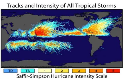
Tropical cyclones (TCs) are the most powerful phenomena of the tropical

atmosphere (instantaneous power of 1012W). They are low-pressure tropical

dis-turbances of more than 1000 km diameter that develop over warm tropical oceans

(Fig. 1.1).Hurricanes in the north Atlantic and northeastern Pacific, typhoons in

the northwestern Pacific ortropical cyclones in the Indian and south Pacific oceans

all refer to the same phenomenon: a rotating, organized system of clouds coupled with the ocean. They are popularly known for their destructiveness causing ca-sualties and material damages to coastal populations. Waiting for solutions to control and use their power, we are left to find solutions to prevent the damages. For example, Australians or Caledonians (Aerowatt company) recently developed wind turbines that can be folded on the ground to prevent their destruction by extreme winds.

Figure 1.1 -Glopbal map of tropical cyclone tracks. Figure from NASA.

As researchers, we can work at a better understanding of the mechanisms of intensification and evolution of tropical cyclones in order to improve their forecast. In recent years, increasing computing power, modeling and observational skills have sustained improvements in the forecast of TC tracks. By contrast, their intensity is still poorly predicted. A probable source of failure is the poor account of ocean structure and dynamics in operational forecasts. The work presented in this manuscript aspire to advance our knowledge of interactions between tropical cyclones and the ocean.

1.1 Generalities on tropical cyclones

1.1.1 Observations

Tropical cyclone observation has been carried out over the past couple of centuries in various ways. Before the satellite era, it was essentially performed by unfor-tunate commercial ships crossing storms. Since World War II, reconnaissance

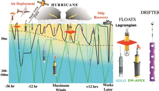
aircrafts called hurricane hunters have been flying out to sea to find tropical cyclones. Nowadays, they provide the most detailed measurements. They use dropwindsondes that are deployed from the aircraft and drift down on a parachute measuring vertical profiles of pressure, temperature, humidity and wind as they fall. However, aircraft deployments are very expensive and only operational in the North Atlantic and North Pacific by American and Japan governments. Since the 1970’s, satellites allow us to observe TCs from space with an increasing space and time coverage. Visible and infrared measurements provides images of the cloud structure and temperature at upper levels, which are representative of the cyclonic circulation, cyclone eye and deep convection. Micro-wave measurements give information on the ocean surface. Scatterometers retrieve the wind direc-tion and intensity and altimeters significant wave height. Satellite and coastal radars provide precipitation rates and patterns. Measurements of oceanic fields and air-sea fluxes can also be retrieved by moorings, Argo autonomous profilers, expendable current profilers or bathythermographs released for a particular event study (for example during the CBLAST, Coupled Boundary Layer Air-Sea Transfer, experiment; Fig. 1.2, Black et al., 2007).

Figure 1.2 -Schematic picture of the instruments deployed into hurricane Frances (2004) during the CBLAST experiment. Figure from Black et al. [2007].

Observations have been very valuable to our understanding of tropical cyclones and are still required, but they are either impracticable or limited. Satellite observations have a good space and time coverage that is very useful for detecting and tracking TCs. However, with a bi-dimensional space coverage, they largely

miss the TC structure and only cover the ocean surface. In situ observations

on the other hand have insufficient space and time coverage. In the absence of a continuous three-dimensional dataset, modeling offers a good alternative to advance our knowledge of tropical cyclones and underlying mechanisms.

1.1.2 General characteristics

Tropical cyclones are deep warm-core structures characterized by organized con-vection, rotating winds, humidity convergence at low-levels and divergence in the upper troposphere (Fig. 1.3). They are maintained by the extraction of heat energy from the warm ocean and are thus part of the marine system; landfall is the end of the cyclone life. Obviously, cyclonic winds inflict a lot of damages to coastal populations before they die as their outer winds can sweep the coast before the eye makes landfall (damages also arise from heavy rain, storm surge and wave set-up and run-up). They can sometimes survive after crossing an island if they are strong and fast enough. Another decaying process is the progression over colder waters and across jet-streams in the subtropics. This is usual as TC trajectory is mainly driven by the mean tropospheric flow that is generally poleward.

Figure 1.3 -Schematic vertical section of TC circulation. Figure from Gray and Emanuel [2010].

Tropical cyclones need specific environmental conditions to develop and main-tain [Gray, 1968]:

• oceanic temperature above 26C over the first 60 m of the ocean, to fuel the

heat engine of the tropical cyclone

• sufficient environmental lapse rate for conditional instability

• high relative humidity at mid troposphere sustaining deep convection • cyclonic absolute vorticity at low level

• weak vertical wind shear preventing vortex disruption and upper dry air intrusion

These conditions are met in tropical convergence zones (Fig. 1.1) where about 80 TCs develop each year. Interestingly, there are no tropical cyclones in the South Atlantic because of strong wind shear and possibly lack of weather disturbances favorable for tropical cyclone initialization [Gray, 1968].

1.1.3 The South Pacific

Figure 1.4 -Austral summer (January-March) mean precipitation in (a) CMAP obser-vations and (b-o) a selection of best CMIP3 climate models in the South Pacific region. The black solid lines represent the SPCZ position in each model. The black dashed line represents the SPCZ position in CMAP observations. Figure from Bador et al. [2012].

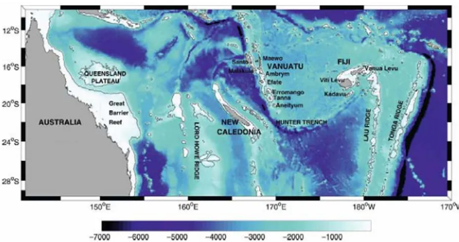
The South Pacific region was chosen for this study in continuation of the work of Jourdain et al. [2011] as part of long-term projects of the IRD (Institut de Recherche pour le Développement). The South Pacific is composed by numer-ous poor islands that are particularly vulnerable to TC activity. It is also largely impacted by the El Niño Southern Oscillation (ENSO) phenomenon. The South Pacific Convergence Zone (SPCZ), which is the only convergence zone of the south-ern hemisphere that is present all year long, is submitted to significant interannual variations due to ENSO with consequences on cyclogenesis. The SPCZ is one of the most poorly simulated convergence zone in climate models (Fig. 1.4) and few studies are dedicated to its understanding. However, the IRD established in Noumea (New Caledonia) for nearly 70 years has dedicated numerous research in the South Pacific (sharing that with Australians) and this thesis is part of the effort.

TC activity in the South Pacific is measured with a different intensity scale than the well-known Saffir-Simpson intensity scale mainly used in the North Atlantic. These scales are reported in Table 1.1. TC intensity is usually represented by

the TC central pressure. The relationship between maximum winds and central pressure for observed TCs in the South Pacific is illustrated in Figure 1.5.

Table 1.1 -South Pacific and Saffir-Simpson intensity scales for tropical cyclones. TS is used for Tropical Storm.

Wind speed South Pacific scale Saffir-Simpson scale

17-24 m/s cat. 1 TS 24-33 m/s cat. 2 TS 33-44 m/s cat. 3 cat. 1 44-55 m/s cat. 4 cat. 2-3 55-70 m/s cat. 5 cat. 3-4 >70 m/s cat. 5 cat. 5

Figure 1.5 -Wind-pressure relationship for observed TCs in the South Pacific (SPEArTC data from 1979 to 1999).

1.2 TC formation and intensification

The genesis and intensification of tropical cyclones has been investigated for decades. Gray [1998] reviewed the processes of tropical cyclone formation. Here, we give a quick summary. Tropical convection forms a variety of mesoscale sys-tems (cloud clusters, mesoscale convective syssys-tems: MCSs) with generally short life span. A strong convective system can develop a mesoscale convective vortex (MCV) that may persist 1 to 3 days after the MCSs die. This residual cyclonic circulation is only about 150-km wide and 5-km deep (Fig. 1.6a) but it has a warm-core with a structure analogous to that of a tropical cyclone and can serve as the nucleus for its formation.

The cyclonic flow associated with the low-pressure center can help organize new areas of convection, but a second external forcing is required to trigger extreme convection (EC; Fig. 1.6a). External forcing can be exerted by wind surges that encounter a convergence line in trade winds or monsoon flow (Fig. 1.7), easterly waves (particularly in the North Atlantic), or other forms of disturbances.

Figure 1.6 -Cross-section view of the steps describing how an externally forced conver-gence (EFC) acts to initiate an area of extreme convection (EC) and the activation of an internally forced convection (IFC), which after a short time of intensification becomes a named storm. Figure from Gray [1998].

The external forced convergence (EFC) must produce an increase in humidity of 20-25% and force the development of extreme convection (EC) in the MCS. It is strong enough to drive air parcels to near saturation and suppress strong downdrafts (1.6b). A larger scale, self-sustained secondary circulation, named internally forced convection (IFC) by Gray [1998], takes place (1.6c). The IFC increases the mass inflow at low-levels from the surrounding environment. At this stage, a tropical cyclone can form. Pressure starts to drop rapidly (5-10 hPa/day)

Figure 1.7 -Schematic picture of the typical organization of cloud clusters in the south-westerly monsoon or trade wind flow. Figure from Gray [1998].

accompanied by a rapid wind spin-up in the inner region. A gradient wind bal-ance between the cloudy area and its environment is established. The pressure gradient towards the storm center maintains the convergence and the TC evolves independently from its environment. One important aspect of this conceptual model is that the development of tropical disturbance must first concentrate on a small inner area with an in-up-and-out radial circulation that allows for a rapid intensification. Then tangential winds out of the core can intensify. An anticy-clonic flow at upper-levels promotes the tangential wind increase out of the core. The intensification also results in strong inertial stability that in turn inhibits the transverse circulation to the core and slows down the intensification.

The conceptual model of Gray [1998] is in essence similar to the Conditional Instability of the Second Kind [CISK; Charney and Eliassen, 1964]. CISK describes the unstable growth of a group of convective clouds which differs by size and time scale from the instability of the first kind that describes the unstable growth of individual cumulus clouds. Charney and Eliassen [1964] suggested that this linear instability process occurs over a 400-500 km area and is initiated by frictionally forced convergence akin to the internally forced convection of Gray [1998].

Fric-tional convergence is analogous to Ekman pumping,i.e., the process of inducing

vertical motions by boundary layer friction. As friction increases with wind speed, frictional convergence is maximum near the radius of maximum winds in the eyewall. Gray [1998] agrees with the concept of CISK but argue that unstable growth can only occur on smaller scales.

Other theories were proposed by Emanuel [1986] and Rotunno and Emanuel [1987] following the idea of a thermodynamical rather than mechanical trigger for deep convection. They suggest that different thermodynamical states exist between disturbances that develop or not into TCs: the developing systems would present higher values of temperature and/or humidity at low-levels. Gray [1998] objects that rawindsonde observations does not indicate systematic differences in temperature and humidity between developing or non-developing disturbances. The Wind-Induced Surface Heat Exchange theory [WISHE; Emanuel et al., 1994]

is a theory of linear instability involving thermodynamical arguments. WISHE is based on the assumption that convection is self-fueling in a coupling process between surface fluxes and winds within the convective system. The TC growth rate is restricted by the magnitude of surface heat and moisture fluxes rather than the frictional convergence mechanism as in CISK [Craig and Gray, 1996]. WISHE has achieved widespread acceptance in the current literature but recent modeling studies have questioned its validity or completeness [Montgomery et al., 2009]. Our work goes along this latter line of research.

A last important aspect of research, of growing interest, is the role of mesoscale interactions in TC formation. The merging of two mesoscale vortices producing a full grown cyclone is relatively rare but has been observed [Kuo et al., 2000] and modeled [Fig. 1.8, Jourdain et al., 2011]. More generally, vortex interaction, from elastic interaction to straining and merger, are ubiquitous aspect of TC formation that should be accounted for [Dritschel, 1995; Guinn and Schubert, 1993].

Obviously, the formation and intensification processes of tropical cyclones are still a matter of research and debate. Tropical disturbances such as wind surges or vor-tex interaction are difficult to forecast because of their chaotic nature. Forecasting generally starts only after the initialization process. The difficulty of forecasting TC intensity is certainly related to the flaw of understanding of intensification processes.

Figure 1.8 -Simulated TC formation by vortex merging. Low-level wind (at 925 hPa) is shown as streamlines and colors (m.s1). Figure from Jourdain et al. [2011].

1.3 Ocean response to TCs

1.3.1 Cold wake formation

Figure 1.9 -SST field and cooling anomaly after the passage of TCs Tomas (black track) and Ului (next to Papua-New-Guinea) in March 2010 retrieve by TMI-AMSR-E satellite data.

The most reported effect of TCs on the ocean is the surface water cooling

observed from satellites where it appears as TCcold wake (Fig. 1.9). The surface

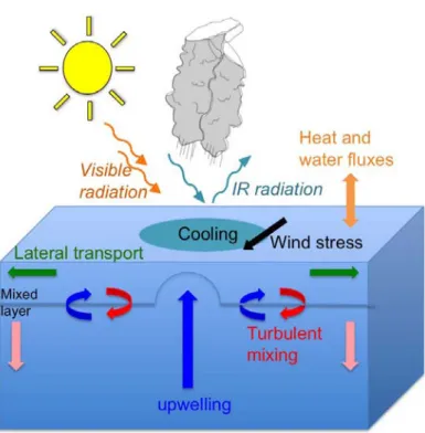
cold wake expresses various storm-induced processes: heat loss to the atmosphere, mixing with subsurface water, upwelling of deep water by Ekman pumping (Fig. 1.11). SST cooling is usually asymmetric because of asymmetric wind

forcing. We define the TC strong side as the side of strongest cooling. On the

strong side, tangential winds and translation speed are added (right-hand side in the Northern Hemisphere and left hand side in the Southern Hemisphere). It is the opposite on the weak side. Asymmetry in winds induces asymmetry in turbulent mixing. In addition, resonance between ocean currents and winds leads to another asymmetric increase in mixing. Translation speed thus has the effect of shifting SST cooling away from the cyclone track [Price, 1981; Samson et al., 2009]. Concurrently, fast translation speed weakens SST cooling (Fig. 1.10). We will show in this thesis that this is largely an effect of supercritical translation speed (with reference to near-inertial phase speed) that weakens the upwelling effect relative to mixing. More detail on the known mechanisms are given below.

1.3.2 Mixing and upwelling mechanisms

Extreme winds in cyclones produce strong mixing of warm surface waters with colder subsurface waters. Mixing is due to both mixed layer entrainment and shear instability associated with near-inertial oscillations, a transitory response to a moving storm [Chang and Anthes, 1978; Shay et al., 1989; Jaimes and Shay, 2009]. Near-inertial motions are characterized by oscillating horizontal and vertical

velocities associated withinertial pumping (Figs. 1.12, 1.13a). Cyclonic rotating

winds also induce an Ekman pumping that is particularly strong for slow or static storms. It is characterized by a very strong upwelling of cold deep water under the cyclone track with weaker and more widespread downwelling on the sides (Fig. 1.13b). In the linear theory, upwelling velocity from Ekman pumping is

Figure 1.10 -Cross-track section profile of SST cooling for different hurricane translation speeds. Figure from Price [1981].

Figure 1.11 -Schematic picture of ocean-atmosphere interactions under a tropical cyclone.

McWilliams, 2006]. Therefore, it strongly participates in the surface thermal response by uplifting the thermocline [Price, 1981; Shay et al., 2000]. Yet, Ekman pumping is generally neglected in conceptual models, at the benefit of the mixing process, as it requires a three-dimensional approach. We will see in this thesis work that Ekman pumping is major player in the cold wake formation.

Figure 1.12 -Cross-track velocity response at a mooring site during hurricane Katrina. Figure from Jaimes and Shay [2009].

Figure 1.13 -TC-induced (a) inertial pumping (104m.s1) and (b) upwelling just below the base of the mixed layer (m) for hurricane Eloise case. Negative values in (a) indicate upward motion, which tends to reduce the mixed layer depth. Figure from Price [1981].

1.3.3 The role of ocean structure and dynamics

Ocean heat transports associated with mixing and upwelling are dependent on upper ocean stratification, which is modulated by surface ocean dynamics. The ocean is structured at different and interacting scales: large-scale, regional scale,

mesoscale and submesoscale. Mesoscale activity,i.e., the formation and evolution

of cyclonic and anticyclonic ocean eddies on the scale of baroclinic deformation radius, shapes the upper thermocline: shallower (deeper) mixed layer is observed for cyclonic (anticyclonic) eddies. The ocean response to TCs over mesoscale

structures were investigated mainly in the Gulf of Mexico [e.g., Bao et al., 2000;

Jaimes and Shay, 2009] where the Loop Current (LC) releases large anticyclonic warm core eddies (WCEs) with positive sea level anomaly and deep mixed layer,

i.e., higher heat content. In this case, it is noticed that mixing produced by

extreme winds is less efficient as a surface cooling process (Fig. 1.14a). On the contrary, a cold core cyclonic eddy (CCE) tends to enhance surface cooling (Fig. 1.14b). Mesoscale eddies are also known for their effect on the efficiency of vertical radiation of near-inertial motions, as their frequency is shifted by the background relative vorticity [Kunze, 1985]. They may even be trapped in the eddy field, enhancing mixing depending on the sign of vorticity [Jaimes and Shay, 2010]. Obviously, upwelling and mixing are complex and interactive processes at multiple scales. Our approach using long-term simulations with realistic models will permit to bring together all this complexity and provide more realistic estimates of their effects.

Figure 1.14 -Upper-ocean temperature profile changes induced by hurricane Rita: (a) in the Loop Current (LC) bulge and (b) in the cyclonic circulation of a growing cold core eddy from airborne profiler clustered data. Figure from Jaimes and Shay [2009].

1.3.4 Impact on the ocean climate

Upwelling is generally considered as a reversible process that has no lasting effect. Yet, vertical advection is a non-linear process interacting with the background flow and may affect the heat and salt budgets over considerable distances. We will see in this thesis that its long-term impact has also been underestimated and misunderstood in previous studies. By contrast, mixing, an irreversible process,

was emphasized for injecting heat below the surface. This process called ocean

2001; Sriver and Huber, 2007). The heat uptake is then assumed available for pole-ward transport by the meridional overturning circulation [Emanuel, 2001]. Based on this idea, TC-induced meridional heat transport was estimated by generally

applying anad-hoc mixing coefficient [Manucharyan et al., 2011] and resulted in

TC contribution to heat transport of 10 to 20%. However, several mechanisms are misconceived in this approach, which we believe largely overestimates the impor-tance of TCs on the climatic scale (see also Vincent et al. [2012c]). First, mixing is a nonlinear process that cannot be simply modeled using scale analysis. Second, ocean heat uptake does not balance SST cooling because of the interaction between mixing and upwelling and because a large amount of this uptake is released back to the atmosphere in winter. These mechanisms and their quantitative effects are analyzed in this work.

Figure 1.15 -Schematic picture of the steps of Emanuel’s hypothesis on TC-induced ocean heat uptake. (a) Strong mixing deepens the mixed layer, creating a cold anomaly at hte top (dotted) and a compensating warm anomaly below (striped). (b) The cold anomaly is removed by net surface enthalpy fluxes. (c) The warm anomaly is removed advectively by buoyancy adjustement to the surrounding ocean. Figure from Emanuel [2001].

1.4 Ocean feedback to tropical cyclones

TC-ocean interactions are essential for cyclone formation and evolution. Ocean heat content is the fuel of TCs. In return, extreme winds inject mechanical energy into the ocean and modify its structure. Modifying the surface ocean heat content, the cold wake has the potential effect of negative feedback on TC

intensity (e.g., Bender et al., 1993; Holland, 1997; Schade and Emanuel, 1999;

Figs. 1.16 and 1.17). Stronger TCs induce stronger cooling that in turn would produce stronger feedback. The question is on the quantification of SST feedback to storm intensity. The thermodynamical theory [Emanuel et al., 1994; Holland, 1997] appears to overestimate the feedback effect compared with observations and realistic modeling case studies. The discrepancy may be related to the assumed intensification process. The WISHE concept implies a large feedback of SST

cooling (Emanuel [1999] suggests that a 2.5◦C cooling could totally shut down

fluxes (more on storm-scale humidity convergence) and implies a weaker feedback effect [e.g., Chang and Anthes, 1979; Sutyrin, 1979]. A better understanding and quantification of ocean-cyclone interactions is therefore required. Our work will provide valuable insights.

Figure 1.16 -SST field and intensity of TC Erica (2003) along its track simulated in (a) forced and (b) coupled ROMS-WRF models. Figure from Lemarié [2008].

Air-sea fluxes are poorly known in general and in particular for extreme events where measurements are impractical. Their evaluation thus remains challenging. Radiative fluxes are better known than turbulent fluxes as they are provided by remote satellite measurements. Usually, turbulent air-sea fluxes are computed using bulk formula that have parameterized exchange coefficients between the ocean and atmosphere for heat, humidity and momentum. The transfer coefficients

known as surface drag coefficient, CD, and enthalpy exchange coefficient, CK, are

the subject of much research [Charnock, 1955; Powell et al., 2003; Donelan et al.,

2004]. The idea is generally to find the best fit to in situ observations for all

situations. However, the variety of sea states and the large range of wind speed make this task difficult. The transfer coefficients for mature swell are generally consensual, but limited fetch young waves and extreme wind conditions can have various and opposite effects. Large and slow (young) waves increase surface roughness and thus the exchange of heat and momentum with negative feedback

on wind speed [Doyle, 2002]. On the other hand, sea-spray,i.e., droplets torn

by extreme winds or produced by breaking waves, promote heat and humidity exchanges as they easily evaporate, leading to increased heat supply to TCs. This represents a positive feedback to cyclonic winds [Bao et al., 2000]. Finally, foam layers act as slipping layers that limit heat and momentum exchanges. As all these processes arise concurrently, the parameterization of exchange coefficients under extreme wind speed conditions is problematic (see also Chapter 6 Section 6.2.2). On the issue of transfer coefficients, we will use a conservative approach (with the Charnock relation) and leave the wave interface coupling for further research. Our objective is focused on the feedback effect of storm-induced SST cooling. This effect is thought as the primary source of interaction between tropical cyclones and the ocean.

Figure 1.17 -Total surface heat flux (kW .m−2(positive value directed upward into the atmosphere) averaged over 72 hours from idealized model experiments (top) with air-sea coupling and (bottom) whithout coupling. Tick marks are 1◦ intervals. Figure from Bender et al. [1993].

1.5 State of the art modeling of tropical cyclones

Tropical cyclone modeling has gradually improved with increasing computing power, more sophisticated models and data assimilation techniques. The large range of scales and processes involved in the tropical cyclone formation and evo-lution and their interaction with the ocean would suggest to use mesoscale or cloud-scale coupled models rather than climate models. However, high-resolution models are complex and still computationally expensive. Until now, only few attempts have been made and they were all based on case studies. Other investiga-tions have used simpler models based on a certain number of assumpinvestiga-tions.

The resolution needed to resolve the TC dynamics and its small scale processes such as convection, vortex Rossby waves and mesovortices is very high. Figures 1.18 and 1.19 show precipitation and vertical velocity fields that can be obtained with different resolution and model configurations. At 35 km resolution, even though small-scale convective processes are parameterized, the overall TC

struc-ture is capstruc-tured, showing eye and eyewall, intense precipitation and rain bands that spirals around. The structure of the vertical velocity field with a tilted eyewall is also correctly represented. The main issue at such mesoscale resolution is that vertical velocities are under-estimated, thus preventing the formation of the most extreme TCs [Gentry and Lackmann, 2009].

Figure 1.18 -Instantaneous precipitation field from Gentry and Lackmann [2009] at 1, 4, 8 km resolution in WRF, from our study at 35 km resolution in coupled WRF-ROMS and in Scoccimarro et al. [2011] at 80 km resolution in a CGCM.

Figure 1.19 -Vertical velocity section composite from Gentry and Lackmann [2009] at 1, 4, 8 km resolution in WRF and from our study at 35 km resolution in coupled WRF-ROMS.

1.5.1 Climate models

The recent attention given to climate change has stimulated the use of global climate models to study changes of tropical cyclone activity in future scenarii.

Yet, global climate models still have insufficient resolution (1◦

or 2◦) to correctly

represent TCs and fail also in some regions to accurately represent the favorable environmental conditions for tropical cyclogenesis. At coarse resolution, models

only produce cyclone-like vortices, which are vortices presenting some

charac-teristics of tropical cyclones but much lower intensities [e.g., Sugi et al., 2002;

Camargo et al., 2005; Scoccimarro et al., 2011]. Their relevance to TC activity remains difficult to assess [Gray, 1998; Camargo et al., 2007]. Increased resolution

at 0.5◦ in more recent global models appears to improve the representation of

cyclones [e.g., Chauvin et al., 2006; Zhao et al., 2009] but the computational cost

of these models limit the number of possible experiments that are needed for tuning the model and for exploring its parameter sensitivity. In addition, the goal of global models is to compute the best global solution at the expense of regional ones. In particular, global models generally fail in representing the South Pacific climate [Zhao et al., 2009; Bador et al., 2012].

To investigate the ocean response to TCs, coarse atmospheric solutions are of poor interest because their underestimated wind magnitude have a corresponding low response in the ocean through mixing and upwelling processes. Pasquero and Emanuel [2008] used the Massachusetts Institute of Technology global ocean

model with 4◦horizontal resolution and 20 vertical levels. They forced the ocean

model with coarse fluxes but added a temperature perturbation over the regions of strong TC activity to simulate their mixing effect. A similarly rough technique was employed by Manucharyan et al. [2011]. The approach is crude, relying on a single process (mixing) that is largely misconceived.

1.5.2 Simple coupled models

Earlier coupled experiments used axisymmetric TC models coupled with a simple

slab ocean mixed layer [e.g., Chang and Anthes, 1979; Sutyrin, 1979]. In a slab

model, the ocean response is controlled by a balance between surface fluxes and entrainment of deep water of pre-defined temperature. Their is no representa-tion here of Ekman pumping or shear instability associated with near-inertial motions. In the TC model, the energy growth rate is balanced by horizontal diffusion and surface friction while the balance of water vapor is achieved by evaporation, horizontal advection and precipitation. Emanuel [1995] designed another type of axisymmetric hurricane model that assumes gradient-wind and hy-drostatic balance. This strongly constrains the vortex structure. Moist convection is represented by a one-dimensional plume whose mass flux is specified to ensure the entropy equilibrium of the boundary layer. This model has the advantage of thermodynamic consistency for assessing the effect of surface heat fluxes on the TC intensity but has oversimplified dynamics for the ocean and atmosphere. An improvement was proposed by [Schade and Emanuel, 1999] using a 3-layer ocean model (mixed layer, thermocline, deep ocean) that allowed internal-wave

dynamics. Before that, Price [1981] also used a 3-layer ocean model but included a representation of Ekman pumping.

1.5.3 Realistic coupled models

Three-dimensional primitive equation ocean models, assuming hydrostatic bal-ance and incompressibility, allow a full description of the ocean heat budget affected by TCs [Price et al., 1994; Huang et al., 2009]. Until now, their use was limited to the study of TC events and focused mostly on surface processes. In chapter 4 of this manuscript we propose a full description of the ocean response to TCs using a similar model but on a great number of events (∼ 200) produced by a 25-year long simulation.

Realistic coupled experiments with 3D ocean and atmosphere models started quite recently. Bender et al. [1993] originally used a simple 3-layer ocean model

coupled with the NOAA-GFDL multiply nested movable mesh (1◦-1/3◦-1/6◦).

They conducted various idealized simulations comparing the feedback effect of SST cooling. More recently, Bender and Ginis [2000] coupled the same atmospheric model with the primitive equations Princeton Ocean Model. They performed 163 nowcasts during the 95-98 North Atlantic cyclonic seasons and showed that the mean absolute forecast error of central pressure could be reduced by about 26% with the coupled model compared with the operation GFDL model.

The effect of waves in realistic coupled models was investigated by Bao et al. [2000]. They coupled the PSU/NCAR mesoscale atmospheric model MM5 (with 45-15km resolution) with the WAve prediction Model (WAM) and the Colorado

University Ocean Model (CUPOM, at 1/5◦resolution). They conducted idealized

experiments over the Gulf of Mexico including the effect of sea spray evaporation and wave age. Sandery et al. [2010] coupled the Bureau of Meteorology’s Tropical

Cyclone Limited area Prediction System (TC-LAPS; at 0.15◦ resolution and 29

sigma levels) and the Ocean Forecasting Australia Model (OFAM; at 1/10◦

resolu-tion and 47 vertical levels) with the OASIS-3.1 coupler. In this case, momentum coupling relies on a so-called inertial relation of surface bulk formulations in the atmosphere and ocean (rather than a transfer of the atmospheric momentum to the ocean). This relation accounts for the waves as a moving reference, not for its effects on the surface drag, which is a weakness of the method. The model was applied on real events of the Australian region.

1.5.4 Long-term regional simulations

Regional models represent a cost-effective alternative for simulating multiple seasons of TC activity. They also benefit from a geographical focus that allows better adjustments of parametrizations, and from the opportunity of controlling lateral inputs. Despite these advantages, few attempts were made at running long-term regional TC simulations.

Long-term regional studies of the South Pacific at mesoscale resolution (30-35 km) were conducted in the South Pacific by Walsh [2004] using the CSIRO Division of Atmospheric Research Limited area Model (DARLAM) and by Jour-dain et al. [2011] using the Weather Research and Forecast model (WRF). These models generate intense TCs, with structures that are often in good agreement with dropsonde data. Spatial and temporal TC distributions are also realistic (at seasonal and interannual timescales). The intensity distribution is good but miss the strongest cyclones (cloud-scale models with resolution of 1-2 km are required for that; see Gentry and Lackmann, 2009), but those are very rare events. Mesoscale configurations have thus the advantage of covering a large range of space and time scales.

Nevertheless, there usage was limited until now to the atmospheric circulation,

neglecting interactions with the ocean,i.e., the feedback from storm-induced SST

cooling. To respond to the challenge, we updated the model configuration of Jourdain et al. [2011] and coupled it to the Regional Ocean Modeling System (ROMS). In doing so, we filled a gap between case studies and coarse resolution climate models.

1.6 Manuscript outline

The objective of the present work is to investigate the coupled mechanisms at play in tropical cyclones. First the oceanic response to TCs, then the ocean feedback are assessed. Contrasting with previous studies of individual events, our analysis is for the first time applied on 20-year realistic simulation of TC activity computed from a regional coupled model of the South Pacific.

Chapter 2 describes in details the coupled model and its configuration, the choice of parametrization and parameter sensitivity experiments. The design of twin coupled and forced simulations that reveals the coupling effects in the analysis is presented, with also the methodology developed to treat the great number (150-200) of simulated TCs.

Chapter 3 presents the South Pacific dynamics and model performances for the regional climate and TC climatology. The seasonal and interannual variability of the South Pacific Convergence Zone and cyclogenesis are assessed and the respective parts of forced and stochastic variability are evaluated.

The impact of TCs on the full 3D ocean heat budget is detailed in Chapter 4. It shows a complete description of the ocean structure changes induced by TC occurrence. The oceanic response is first addressed at the cyclone scale before assessing its lasting effect on the ocean climatology. The use of a composite method representing the average of all simulated TCs highlights the most robust features of their effect.

The ocean feedback on TCs is finally studied in Chapter 5. It presents the modification of air-sea fluxes by SST cooling and associated reduction of the TC heat supply. The role of the oceanic structure and dynamics in modulating the ocean feedback to TCs is examined. Regional patterns of coupling sensitivity are deducted. Finally, TC intensification theories are discussed in the view of our results.

Chapter 6 summarizes the conclusions and novel results of the thesis. We then propose future directions for the continuation and application of this work.

Chapter

2

Development of a coupled model for

the South Pacific

Contents

2.1 Models

. . . 26 2.1.1 Atmospheric model: WRF . . . 26 2.1.2 Ocean model: ROMS. . . 29 2.1.3 Coupler . . . 31

2.2 Sensitivity tests

. . . 35 2.2.1 Convection . . . 35 2.2.2 Planetary boundary layer (PBL) . . . 37 2.2.3 Cloud microphysics . . . 38 2.2.4 Shortwave radiation . . . 38 2.2.5 Surface drag . . . 39 2.2.6 Skin SST . . . 41 2.2.7 Land surface model . . . 42 2.2.8 Sponge layers . . . 43 2.2.9 Sensitivity to vertical resolution . . . 43

2.3 Methodology

. . . 43 2.3.1 TC tracking and SPEArTC database . . . 43 2.3.2 Forced model: cold track filtering technique . . . 47 2.3.3 Statistics and error bars . . . 49 2.3.4 Compositing methodology . . . 53

Our objective is to analyze the ocean-atmosphere coupling processes that influence tropical cyclonic activity and the ocean response to this activity. We propose a statistically robust approach using long-term simulations of the South Pacific present climate that produce a great number of tropical cyclones (150-200 TCs). This requires a coupled model of the South Pacific region with good capabilities in simulating the present climate at large scale and at cyclone scale. To that end, we developed a coupled framework that was submitted to numerous sensitivity tests to select the best set of parameters and parameterizations for the representation of the regional climate and cyclonic activity. The coupled system and sensitivity experiments are described in this chapter. Some statistical methods to assess error bars in our model solutions will also be presented.

2.1 Models

2.1.1 Atmospheric model: WRF

The regional Weather Research and Forecast model (WRF) was chosen for this study in continuation to the work of Jourdain et al. [2011]. It is a three-dimensional regional community model that resolves compressible, non-hydrostatic Euler equa-tions. We use the Advanced Research WRF (ARW) dynamic solver [Skamarock and Klemp, 2008] as it was specially designed with high-order numerical schemes to enhance the model’s effective resolution of mesoscale dynamics [Skamarock, 2004] which is the point of our study. WRF also includes a large set of parameteri-zations that can be selected and adjusted for a given problem. It is widely used all over the world as it provides, in addition to state-of-the-art methods, great support from developers and the whole users community. New releases of the model are regularly (almost every year) proposed. We chose the version 3.3.1 as it was the latest release available at the beginning of my work, but updated from the version 2.2 used in Jourdain et al. [2011]. As parametrization schemes can change from one release to another, it was necessary to test again the chosen set of parameterizations and eventually adjust some parameters to correctly represent the regional dynamics.

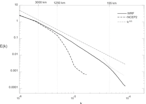
The WRF simulation of Jourdain et al. [2011] were analyzed to present the climatology and interannual variability of South Pacific TC distribution (this simulation will be used to force our ocean model in the first part of the results of the thesis). They evaluated the effective resolution of the model for a 35-km grid resolution. The effective resolution of a model can be defined as the scale at which the model kinetic energy spectrum decays relative to the expected

spec-trum [Errico, 1985; Skamarock, 2004] which is the k−5/3Kolmogorov scaling law

describing motions at scales below 1000 km. Figure 2.1 shows that the model effective resolution is 155 km (break in the slope) that is 5 times the grid resolution. This is finer than most of mesoscale convective systems (∼ 250 km) from which tropical cyclones form [Gray, 1998].

At the boundaries of the regional model, forcing from the 6-hourly National Centers for Environmental Prediction Reanalysis 2 [NCEP-2 reanalysis; Kanamitsu et al., 2002] is applied. Figure 2.1 shows also that NCEP-2 effective resolution is 1250 km and that the NCEP2 forcing conditions are properly passed down to WRF since the spectra obtained for WRF and NCEP-2 are very similar for scales larger than 3000 km.

Figure 2.1 -1981 summer (January-March) wavenumber spectra of surface kinetic energy for WRF model (solid bold curve), NCEP2 reanalysis (dashed bold curve) and theoric Kolmogorov law (dotted-dashed curve). The kinetic energy E is in Joules, the wavenumber

k in m−1. Figure from Jourdain et al. [2011]

The regional domain of simulation encompasses the Indo-Pacific region (89.83◦

E-240.18◦E/41.21◦S-21.62◦N) in order to properly resolve mesoscale activity around

the convergence zones (Inter Tropical convergence Zone, ITCZ, and South Pacific Convergence Zone, SPCZ). Our experience is that boundary forcing located too close to these zones introduces strong biases. A two-way nesting is used to refine the resolution in the region of interest (southwest Pacific) and limit the compu-tational cost. The parent domain has a 105-km resolution and the child domain

(139.62◦E-200.02◦E/31.40◦S-1.62◦S) 35-km resolution (Fig. 2.2). This 3:1 ratio

is generally recommended for nesting as it avoids sharp changes of scales and dynamic regimes across embedded grids. Two-way nesting consists in (at each model time step of 300 s): computation of the parent solution; interpolation of parent solution on the lateral boundaries of the child domain; advancing the child solution for 3 time steps (100 s each); providing a feedback of the child solution

to the parent grid (i.e., interpolated at the parent domain resolution) for the next

computational time step of the parent domain.

The model uses a C-grid (Fig. 2.3) with 31 terrain-following vertical levels with refinement in the planetary boundary layer (PBL) and in the upper troposphere

(Fig. 2.3). Other vertical resolutions and refinements have been tested and are presented in section 2.2. 90oE 120oE 150oE 180oW 150oW 120oW 36oS 24oS 12oS 0o 12oN Australia

Papua New Guinea

New Caledonia Vanuatu

Wallis & Futuna

Figure 2.2 - Simulation domain. Shading represents the terrain height. The rectangle black box represents the limits of the child domain.

Figure 2.3 -(a) C-grid of the WRF model with nesting. The red arrow points to the (i, j) position of the nest in the parent domain. (b) Distribution of the 31 vertical levels in our WRF configuration.

The configuration and choice of parametrization is very similar to that of Jourdain et al. [2011] and was selected to realistically represent the large-scale environment and related tropical cyclone activity in the Southwest Pacific. The details of the whole set of parameterizations used can be found in the model namelist and parameterization short description (see Appendices A and B). Physi-cal parametrizations include the Betts-Miller-Janjic (BMJ) convective scheme; the Yonsei University (YSU) planetary boundary layer (PBL) with Monin-Obukhov surface layer parameterization; the WRF single-moment three-class microphysics scheme (WSM3); the Dudhia shortwave radiation scheme; and the Rapid Radia-tion Transfer Model (RRTM) for longwave radiaRadia-tion. The surface drag coefficient

is given by the classical Charnock relation. Sensitivity tests on these

parame-terizations are presented in section 2.2 as some of the schemes (e.g., BMJ) were

significantly updated since version 2.2.

2.1.2 Ocean model: ROMS

The ocean model used is the Regional Oceanic Modeling System [ROMS; Shchep-etkin and McWilliams, 2005]. ROMS solves the primitive equations in an Earth-centered rotating environment, based on the Boussinesq approximation and hy-drostatic vertical momentum balance. In this study, we use the ROMS-AGRIF version of the model that has two-way nesting capability (not used here) and a compact package for implementation of realistic configurations [Debreu et al., 2012]. It is a split-explicit, free-surface ocean model, discretized in coastline- and terrain-following curvilinear coordinates using high-order numerical methods for reduction of small-scale numerical dispersion and diffusion errors. Associated with a 3rd-order time stepping, a 3rd-order, upstream-biased advection scheme allows the generation of steep gradients, enhancing the model’s effective resolu-tion [Marchesiello et al., 2011]. Because of the implicit diffusion in the advecresolu-tion scheme, explicit lateral viscosity is unnecessary, except in sponge layers near the open boundaries where it increases smoothly close to the lateral open boundaries. For tracers, a 3rd-order upstream-biased advection scheme is also implemented but the diffusion part of this scheme is rotated along isopycnal surfaces to avoid spurious diapycnal mixing and loss of water masses [Marchesiello et al., 2009; Lemarie et al., 2012].

The turbulent vertical mixing parameterization is based on the scheme pro-posed by Large et al. [1994], featuring a K-profile parameterization (KPP) for the planetary boundary layer connected to an interior mixing scheme (see section 4.6 for details). The boundary layer depth (h) varies with surface momentum and buoyancy forcing and is determined by comparing a bulk Richardson number to a critical value. The surface layer above the oceanic boundary layer obeys the similarity theory of turbulence. At the base of the boundary layer, both diffusivity and its gradient are forced to match the interior values. Below the boundary layer, vertical mixing is regarded as the superposition of three processes: verti-cal shear, internal wave breaking, and convective adjustment. The KPP model has been shown to accurately simulate processes such as convective boundary layer deepening, diurnal cycling, and storm forcing: it is widely used in ocean

modeling [e.g., Halliwell et al., 2011]. The model has also shown a reasonable

level of accuracy in modeling TC-induced mixing [Jacob and Shay, 2003]. Some processes are nevertheless missing in this parameterization: for example, mixed layer instabilities that would further help the restratification process in the TC

wake [Boccaletti et al., 2007] are neither resolved in our 1/3◦ resolution model nor

parameterized [for tropical applications, see also Marchesiello et al., 2011]. Open boundary conditions are treated using a mixed active/passive scheme [Marchesiello et al., 2001] that forces large-scale information from the Nucleus for

European Modeling of the Ocean (NEMO) global model while allowing anomalies to radiate out of the domain. The use of similar ROMS configurations in the south-west tropical Pacific region is largely validated through studies demonstrating skills in simulating both the surface [Marchesiello et al., 2010b] and subsurface ocean circulation [Couvelard et al., 2008].

Two different configurations of the ocean model are used along this thesis. The first one was used to study the ocean response to TC forcing. It is a 25-year

(1979-2003) forced ocean simulation with NEMO 1/2simulation forcing at the

boundaries [described in Couvelard et al., 2008] and 41 terrain-following vertical levels with 2-5-m vertical resolution in the first 50 m of the surface and then 10-20-m resolution in the thermocline and 200-1000-m resolution in the deep

ocean. The horizontal resolution is 1/3, and the baroclinic time step is 1 h; hourly

outputs are stored for a case study and 1-day- averaged outputs are stored for long-term analysis. In this first configuration The modeled domain is quite the

same as the child domain of the atmospheric model (140E-190E/30S-8S, Fig.

2.4).

The second configuration is 20-year long simulation (1979-1998) coupled with WRF to study the feedback effect of storm-induced SST. It has 51 terrain-following vertical levels with 2-5 m resolution in the first 50 m, 10-20 m resolution in the thermocline and 50-250 m in the deep ocean. The oceanic domain is the same as

the inner atmospheric domain (139.62E -200.02E /31.40S -1.62S ) with the

exact same grid and same 35-km horizontal resolution (no interpolation is needed to transfer data between the ocean and atmosphere). The interannual oceanic

forcing is from the ORCA025 (NEMO 1/4) global oceanic model simulation

[Barnier et al., 2006] and applied at open boundaries with the mixed active/passive conditions described above.

Figure 2.4 -Oceanic geography of the southwest Pacific. Shading is the ocean depth. Figure from Couvelard et al. [2008].

2.1.3 Coupler

2.1.3.1 Coupling methodology

The procedure of ocean-atmosphere coupling is not straightforward as it requires to ensure a continuity of heat and momentum fluxes at the air-sea interface. Two usual coupling approaches can be found. For global configurations [Bryan et al., 1998], it is based on the exchange of averaged-in-time fluxes on a given time window (between 1 hour and 1 day depending on the application and the need to resolve the diurnal cycle; Fig. 2.5). Over this time window, both models are forced by exactly the same mean fluxes which ensures strict conservation of the quantities. However, the models are not in exact balance as the modification of the ocean state does not feed the atmosphere model on the proper time window but only on the next one. This is thus only an approximation of the mathematical coupling problem and suffers from synchronization issues that may lead to a form of numerical instability [Lemarié, 2008; Lemarie et al., 2013].

Figure 2.5 -Schematic picture of the coupling by time window.

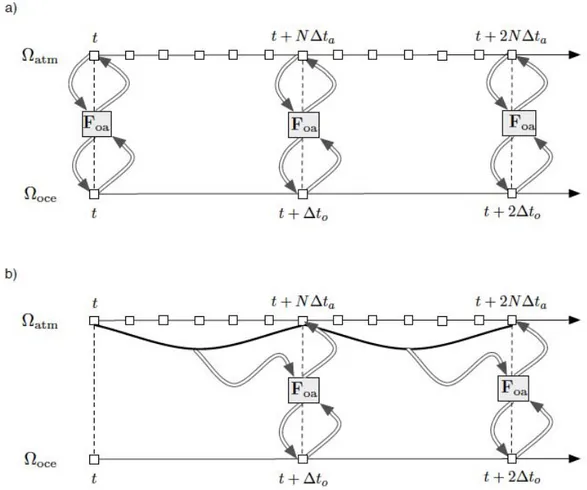
For regional configurations using high-resolution grids [Perlin et al., 2007; Bao et al., 2000], the coupling is usually achieved by the exchange of instantaneous fluxes on the larger model time step (usually the ocean model time step, Fig. 2.6a). It is also possible to exchange integrated atmospheric fluxes over the coupling time step (Fig. 2.6b). This method has less synchronization issues (this method is sometimes referred to as synchronous) but may raise some conservation problems [Lemarie et al., 2013]. More importantly perhaps, the method is mathematically sound only if the coupling time step is small enough to represent the continuous exchange of fluxes between the ocean and the atmosphere. However, the sign of turbulent fluxes, involved in the computation of air-sea fluxes, can be uncertain on time scales less than 10 minutes and hourly fluxes are more relevant [Large, 2006]. This is explained by the lack of accurate knowledge and direct observations of fine-scale air-sea fluxes. Moreover, the empirical transfer coefficients involved in bulk formulations are calibrated through mean hourly measurements. To partly alleviate this problem, additional physical processes can be implemented in bulk formulations that are relevant to high-frequency coupling or extreme conditions.

For tropical cyclones, relevant processes involves sea-spray contributions and wave age factors to turbulent exchanges in the wavy boundary layer [Bao et al., 2000]. In this case, it can be assumed that uncertainties in bulk fluxes are reduced and instantaneous fluxes may become more relevant. However, more research is needed in this direction.

Lemarié [2008] has proposed a compromising approach for synchronous cou-pling based on the time window framework. The method uses a global in time Schwarz method that consists in iterating the coupling procedure at each time step until flux computation converges. More specifically, the coupling algorithm, schematized in Figure 2.7, consists in the following steps:

1 Advancing the atmospheric solution on a given time window (coupling

fre-quency), using the ocean model SST of the last time window (or the initial SST field at initialization).

2 Computing averaged surface momentum, heat and fresh water fluxes over the

time window

3 Advancing the ocean model for the same time window using surface fluxes

computed at step 2 for model forcing.

4 Advancing again the atmospheric model on the same time window using the

ocean model SST computed at step 3 and computing again the averaged surface momentum, heat and fresh water fluxes over the time window

5 Comparing the fluxes computed at step 2 and 4 to evaluate the convergence

(convergence is reached when the difference between computed fluxes is lower than a given threshold).

This algorithm ensures synchronization and a strict conservation between models. On the other hand, the iterative procedure considerably increases the computational cost of the coupling, especially when the convergence is slow. Lemarie et al. [2013] evaluates the performance of the coupling algorithm on the Erica tropical cyclone case in the South Pacific. They found that 3 iterations of the coupling algorithm was enough for convergence and to get rid of the nu-merical instability arising from synchronization lost. In our study, the need of long-term simulations prevents the use of an iterative process that multiplies by 3 our computational cost (see section 2.1.3.2). However, a compromise was found by reducing the coupling time window to 3 hours, which put us in a middle ground between synchronous and asynchronous methods. We performed sensitivity tests

that compared the number of coupling iterations (1vs.3 iterations) and found no

particular improvement with the 3-iteration experiment. We conclude that the time window is small enough to prevent the numerical instability described by Lemarie et al. [2013], at least most of the time.

As a result of our experiments, we choose to use the coupler of Lemarié [2008] with only one iteration. This is equivalent to use the global-in-time coupling

Figure 2.6 -Example of two coupling strategies at the time step level. toand tadenote the

(baroclinic) time steps respectively of the ocean and the atmosphere model, with to= N ta

(N = 6 here). The arrows represent an exchange of information with the surface layer parameterization function Foa. For the atmospheric component, this exchange is based on

instantaneous values in algorithm a) and on time-integrated values in b). From Lemarie et al. [2013].

Figure 2.7 -Schematic picture of the iteration process to evaluate convergence in the Schwarz algorithm. Figure from Lemarie et al. [2013].