Descriptive and explanatory tools for human movement and state estimation in humanoid robotics

(1)

THÈSE

En vue de l’obtention du

DOCTORAT DE L’UNIVERSITÉ FÉDÉRALE

TOULOUSE MIDI-PYRÉNÉES

Délivré par :

l’Université Toulouse 3 Paul Sabatier (UT3 Paul Sabatier)

Présentée et soutenue le 10 octobre 2018 par :

❋r❛♥ç♦✐s ❇❆■▲▲❨

Descriptive and Explanatory Tools for Human Movement and State Estimation in Humanoid Robotics

JURY

Laurence CHÈZE _{Professeure des Universités} _Rapporteur

Auke IJSPEERT _Professor _Rapporteur

Jean-Paul LAUMOND _{Directeur de Recherche} _Examinateur

Emmanuel GUIGON _{Chargé de Recherche} _Examinateur

Philippe SOUÈRES _{Directeur de Recherche} _{Directeur de Thèse}

Bruno WATIER _{Maître de Conférence} _{Co-directeur de Thèse}

École doctorale et spécialité : EDSYS : Robotique 4200046 Unité de Recherche :

Laboratoire d’Analyse et d’Architecture des Systèmes, LAAS-CNRS Directeur(s) de Thèse :

Philippe SOUÈRES et Bruno WATIER Rapporteurs :

(2)

(3)

i

Remerciements

J’adresse ces remerciements à mes encadrants, Philippe Souères et Bruno Watier, pour m’avoir offert l’opportunité de travailler sur les différentes questions abordées dans ce document. En particulier, je suis reconnaissant à Bruno d’avoir motivé la partie biomécanique du travail présenté, contribuant à son aspect pluridisciplinaire qui m’est cher. Ensuite, je veux chaleureusement remercier Philippe pour avoir su, il y a trois ans, me proposer un projet de thèse original que nous avons affiné au cours de nombreux échanges passionnants. Ils ont aiguisé ma curiosité, ma rigueur et mon goût pour la recherche et ils constituent le terreau des résultats qui ont vu le jour lors de cette thèse.

Je tiens à remercier Laurence Chèze et Auke Ijspeert pour leurs relectures attentives et les rapports motivés qu’ils ont fournis sur ce document. Je remercie également tous les membres du jury d’avoir fait le déplacement pour assister à la présentation du travail de cette thèse.

Le travail présenté ici n’aurait jamais vu le jour sans le soutien scientifique, technique et humain de l’équipe GEPETTO. Je souhaite remercier chacun de ses membres, des temporaires aux permanents, collègues et amis, qui constituent un ensemble riche au sein duquel il est très agréable d’évoluer et d’échanger. Parmi eux, j’ai eu la chance de collaborer plus étroitement avec Galo Maldonado et Justin Carpentier, que je tiens à remercier pour le temps passé à travailler ensemble.

Finalement, je remercie ma famille et mes amis d’avoir fourni des avis extérieurs pertinents sur ce travail et d’enrichir mon quotidien de leur présence.

(4)

(5)

3.2 Mathematical background . . . 44 3.3 Experimental identification of dc−∆ . . . 44 3.3.1 Participants . . . 45 3.3.2 Experimental protocol . . . 45 3.3.3 Data acquisition . . . 47 3.3.4 Statistics . . . 47 3.3.5 Experimental results . . . 48 3.3.6 Discussion . . . 49 3.3.7 Conclusion . . . 49

3.4 Humanoid robot trajectory generation . . . 50

3.4.1 General overview of the motion generation pipeline . . . 52

3.4.2 Centroidal optimal control formulation . . . 52

3.4.3 Simulation results . . . 53

3.4.4 Discussion . . . 53

3.5 Conclusion & perspectives . . . 54

4 On the coordination of highly dynamic human movements An extension of the Uncontrolled Manifold approach applied to precision jump in parkour 57 4.1 Notions of motor control . . . 58

4.1.1 Motor redundancy . . . 58

4.1.2 Hierarchies of motor tasks . . . 59

4.1.3 The Uncontrolled Manifold approach . . . 59

4.1.4 Contribution to the field . . . 61

4.2 Extending the uncontrolled manifold approach . . . 61

4.2.1 Mathematical formulation of the UCM approach . . . 61

4.2.2 Extending the UCM approach to dynamic tasks . . . 62

4.2.3 An application to linear and angular momenta derivative tasks 65 4.3 Application to Take-off and Landing Motions in Parkour . . . 65

4.3.1 Precision jump and landing in parkour . . . 66

4.3.2 Experimental materials and methods . . . 66

4.3.3 Hypothesized task functions . . . 68

4.4 Results . . . 70

4.4.1 Take-off . . . 70

4.4.2 Landing . . . 71

4.5 Discussion . . . 73

(7)

Contents v

4.6 Conclusion and Perspectives . . . 75

III From centroidal state estimation in engineering to state observation in animals 79 5 State estimation for systems in contact Recursive estimation of the center of mass position and angular momentum variation of the human body 85 5.1 Introduction . . . 85

5.1.1 State of the art . . . 86

5.1.2 Contribution . . . 86

5.2 Methods . . . 87

5.2.1 Estimated variables coupling . . . 87

5.2.2 Measurements . . . 88

5.2.3 Multi-source estimation of the CoM position . . . 88

5.2.4 Multi-source estimation of the angular momentum variation quantity . . . 90

5.2.5 Recursive estimation of the CoM position and the angular momentum variation . . . 92

5.3 Experimental validation of the estimation framework . . . 93

5.3.1 Generation of ground truth and noisy measures in simulation 93 5.3.2 Application to human data . . . 96

5.4 Discussion . . . 98

6 State estimation for systems in contact Using Differential Dynamic Programming for optimal centroidal state estimation 101 6.1 Introduction . . . 101

6.2 State of the system and motivations . . . 102

6.3 System’s state observation . . . 103

6.4 Estimating the state . . . 104

6.4.1 State transition and observation equations . . . 104

6.4.2 Problem formulation . . . 104

6.4.3 The DDP algorithm . . . 108

6.5 Illustration . . . 109

6.6 Perspectives . . . 110

7 Should mobile robots have a head ? A rationale based on behavior, automatic control and signal processing115 7.1 Introduction . . . 116

7.2 The Head in animals . . . 119

(8)

7.3.1 State space representation and control of a multi-joint mobile

robot. . . 121

7.3.2 The observation problem. . . 122

7.3.3 Head morphology and exteroceptive sensors. . . 124

7.4 A Head for signal processing and cognition . . . 124

7.4.1 Centralizing exteroceptive perception and its processing. . . . 124

7.4.2 Shortening of the brain-ESO transmission channel. . . 125

7.4.3 Stiffening the exteroceptive kinematics. . . 125

7.4.4 Head mobility for enhanced perception . . . 125

7.5 The role of the head in locomotion and manipulation . . . 126

7.5.1 The head at the front-end of the movement for locomotion. . 126

7.5.2 One Head for supervising manipulation . . . 127

7.6 Conclusion . . . 127

Conclusion and perspectives 131

A Calculation details of the UCM extension applied to kinematic and

dynamic task functions 135

B Application of the UCM extension to the derivative of the

centroidal momenta task functions 137

(9)

List of Figures

1 Vitruvian man, pen and ink with wash over metalpoint on paper,

Leonardo Da Vinci, circa 1490. . . . 2 2 Five deer heads in the Nave region of Lascaux cave that might

represent a single deer at different stages of its motion [Azéma 2012]. Reproduction of a Paleolithic drawing in the Lascaux cave, Musée d’Aquitaine, France. This is one of the first known illustration of animals in motion, where artists seemed to have captured the notion of displacement that is an elementary component of motion. . . 4 1.1 Chronophotograph of a flying pelican. Étienne-Jules Marey, 1882. . 13 1.2 Anatomical posture, from [Whittle 2007]. . . 15 1.3 Locations of anatomical landmarks selected by [McConville 1980,

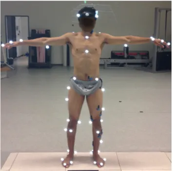
Young 1983] and orientations of coordinate systems attached to these landmarks. From [Dumas 2007]. . . 16 1.4 Example of anthropometric table. From [Dumas 2007]. . . 19 1.5 Volunteer participant equipped with infrared markers fixed onto

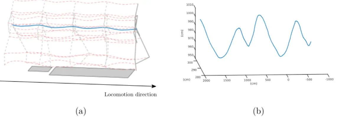
anatomical landmarks. Courtesy of G. Maldonado. . . 20 1.6 (a). 3D plots of the CoMs of each segment (in dashed red) and of

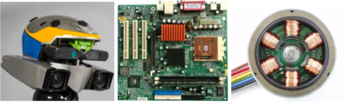
the global CoM (in blue) during a walking movement on horizontal ground. (b). Emphasis on the global CoM during the same motion. . 21 2.1 Technical parts representing the three cornerstones of robotics:

perception, decision and action. Head of the humanoid robot HRP-2 at LAAS-CNRS carrying multiple sensors for multimodal perception

(left). Motherboard that holds and allows communication between

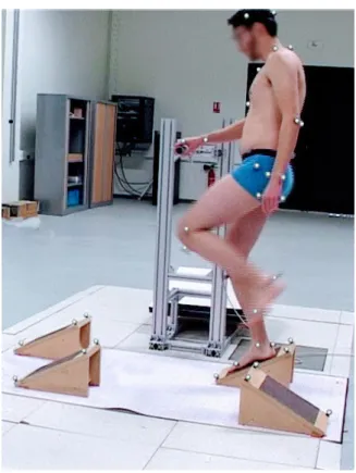
the central processing unit and the memory, and that provides connectors for other peripherals such as sensors and motors (middle). Brushless DC electric motor, the most prevalent example of actuator in mobile robotics (right). . . 27 2.2 Schematic modeling of an open-loop dynamic system. . . 29 3.1 Overview of the experimental setup during a recording session. A

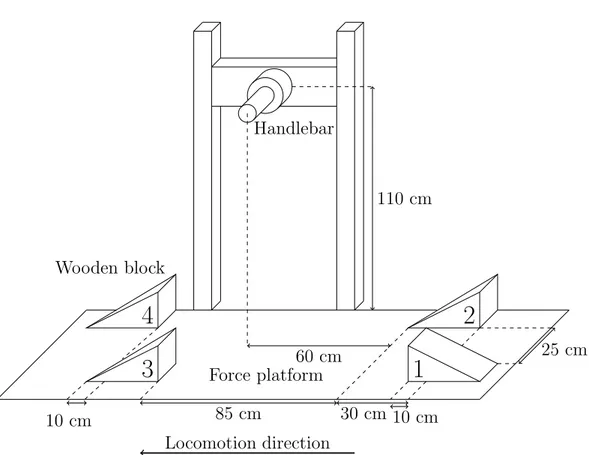
participant is asked to achieve a challenging locomotion task while using the handlebar to help himself. . . 43 3.2 Scheme of the experimental setup with the range of distances

considered. The scenario is composed of four tilted and adjustable wooden blocks. Each wooden block is topped with an adherent layer to prevent subjects from slipping. . . 45

(10)

3.3 Illustration of the different measurement involved in the experiment.

ffp is the force recorded from the force platform, fh is the force recorded from the handlebar, m is the global moment expressed at the center of the force platform. ∆ is the central axis of the external contact wrench. The dashed curved line is the path of c in time.

dc−∆ is highlighted in the magnified portion of the image. . . 46 3.4 Normalized walking cycle in condition A (walking on flat ground).

A: dc−∆in mm as mean ± std, for the 15 participants. B: Height (z component) of the right and left toe markers for one participant. . . 48 3.5 Snapshots of the 15-cm steps climbing motion with handrail by the

HRP-2 robot in simulation. . . 50 3.6 Traces representing the distance dc−∆in the two cases of study: with

and without regularization of dc−∆. . . 51 3.7 Traces representing the control input (acceleration of the CoM and

the angular momentum variations expressed at the CoM) that drives the centroidal dynamics in the two cases of study: with and without regularization of dc−∆. . . 51 3.8 Traces representing trajectories of the state of the centroidal

dynamics in the two cases of study: with and without regularization of dc−∆. . . 51 4.1 The word parkour derives from the classic obstacle course method

of military training proposed by Georges Hébert (Parcours du

Combattant in French). Here are displayed the five steps of the jump

from Hébert’s Méthode Naturelle. . . . 57 4.2 What does it take not to fall from this wobbly structure, while

keeping bowls balanced on your head? At least, three tasks are executed in parallel: keeping the body balanced on the unstable setup, maintaining the balance of the stack of bowls by controlling the head, all this while modifying the body configuration to grab another bowl. Craig Nagy, Wikimedia Commons, CC BY-SA 2.0. . 60 4.3 Experimental setup and motion analysis for the parkour precision

technique. (a) The highest and the lowest two skeletons illustrate the beginning and the end of the take-off and of the landing motion, respectively. (b) Vertical trajectory of the CoM during the whole motion. (c) Vertical reaction force profiles during the whole motion.

From [Maldonado 2018a]. . . 67

4.4 Mean (± confidence intervals) values of the indexes of task control (ITC) during the take-off motion for the LMD(y,z) and the AMD(y) task functions, at each selected phase (1, 40, 70 and 100%.) Below: corresponding snapshots of the reconstructed motion. From

(11)

List of Figures ix

4.5 Mean (± confidence intervals) values of the indexes of task control (ITC) during the landing motion for the LMD(z), LMD(x,y) and the AMD(x,y,z) task functions, at each selected phase (4, 13, 20, 40 and 100%.) Below: corresponding snapshots of the reconstructed motion.

From [Maldonado 2018a]. . . 72

5.1 Illustration of the measurement apparatus. The several physical quantities involved in the estimation framework are displayed, as well as a simplified sketch of the estimation framework. . . 87 5.2 Schematic representation of the spectral accuracy of the different

input signals involved in the estimation of c and ˙Lc. . . 91 5.3 Flow chart for the recursive complementary estimation framework.

s is the Laplace variable. Dotted lines represent the update step of

the algorithm. Complementary filtered components are summed up in order to output ˙Lest

c and cest, estimates of ˙Lc and c respectively. 92 5.4 Norm of the error integrated over the whole trajectory for the

different estimates of c in simulation, as a function of estimation steps. . . 94 5.5 Different contributions to the estimates of c and ˙Lc in simulation.

First row: cforce _{high-pass filtered, c}mocap _{band-pass filtered.} Second row: true c, cmocap_{, c}axis _{low-pass filtered and c}est_{. Third} row: Logarithm of the norm of the FFT of the error for the different estimates. Fourth row: ˙Lest

c and ˙Lc. . . 95 5.6 Different contributions to the estimates of c and ˙Lc on human

recorded data. First row: cforce_{high-pass filtered, c}mocap_band-pass filtered and caxis _{low-pass filtered. Second row: c}est _{and c}mocap_. Third row: ˙Lest

c . . . 97 6.1 (Left) Logarithm of the total cost to go as a function of iterations of

the DDP. (Right) Logarithm of ∇ωiQi as a function of iterations of

the DDP. . . 109 6.2 Three components of c, p and ˙p . . . 111 6.3 Three components of Lcand ˙Lc. . . 112 7.1 Kingfisher in the wind. These pictures are extracted from a short

video clip of the bird fishing. The kingfisher’s head remains still, while its body, attached to a swaying blade of grass, moves and deforms in all directions. The red dot is fixed in the frame of the camera, showing the anchorage of the head with regard to an inertial frame, despite the external perturbation applied to the bird’s body. . 116 7.2 Examples of anterior structures in different bilateral animals

highlighting their heads, sensory and trophic systems. From left to right: Zygoptera, Sepiida, Felidae (Panthera lineage), Callitrichinae, Gekkota, Tetraodontidae, Culicidae, Casuarius. . . 117

(12)

7.3 Artist’s impression of the fauna at the Ediacaran–Cambrian boundary. Different kinds of morphotypes are illustrated as well as their feeding behaviors. © Agathe Haevermans. . . 118 7.4 Three different multi-joint mobile robots at LAAS: the flying

manipulator Aeroarm (left), the mobile manipulator Jido (center), and the humanoid robot Talos (right). The usual choices for their root frame placement are displayed. . . 121 7.5 Illustrations depicting the internal and external states of a simple

polyarticulated robot. (a): Absolute parameterization of the system in the plane. (b): Between the three cases depicted, only the external state of the system is changed. (c): The external state is parametrized by fully positioning the first body. (d): The parameterization of the external state is distributed on the three bodies of the robot. . . 123

(13)

List of Tables

1.1 Definitions of anatomical landmarks of Fig. 1.3, from [McConville 1980]. . . 17 3.1 Distances between the central axis of the external contact wrench

and c, and average locomotion speeds across conditions A, B, C, D and E. Data are expressed as mean ± SD. Superscript ⋆ (resp. †) stands for “Not significantly different from conditions C (resp. E)". . 46 4.1 ITC-based hierarchical organization of the task functions during the

take-off motion. ∗ stands for AMD(y) ITC significantly different from LMD(y,z) ITC. . . 71 4.2 ITC pairwise comparisons using paired t-tests for the task factor

during the landing phases. p−values are adjusted with the Bonferroni correction. . . 73 4.3 ITC pairwise comparisons using paired t-tests for the phase factor

during the landing phases. p−values are adjusted with the Bonferroni correction. . . 73 4.4 ITC-based hierarchical organization of the task functions during the

landing motion. ∗, † and ‡ stand for significantly different from LMD(x,y), AMD(x,y,z) and LMD(z), respectively. . . 73

(14)

(15)

Glossary

∆ Central axis of the contact wrench

Lc Angular momentum at the center of mass

c Center of mass

p Linear momentum

dc−∆ Distance between the CoM and ∆ A-P Antero-Posterior

AMD Angular Momentum Derivative

CMOS Complementary Metal Oxide Semiconductor CNS Central Nervous System

CoM Center of Mass CoP Center of Pressure

DDP Dynamic Differential Programming DoF Degree of Freedom

ECW External Contact Wrench EMG Electromyography

ESO Exteroceptive Sensory Organ IMU Inertial Measurement Unit ITC Index of Task Control

LMD Linear Momentum Derivative M-L Medial-Lateral

MoCap Motion Capture

SCS Segment Coordinate System STA Soft Tissue Artifact

UCM Uncontrolled Manifold ZMP Zero Moment Point

(16)

(17)

Preamble

Measuring and portraying the human body is an old scientific and philosophical matter that goes back to Antiquity. One of the earliest and most remarkable example of the human will to describe its own body thanks to geometry appeared in Vitruve’s treatise, De Architectura. Leonardo Da Vinci, later reproduced this description of ideal human proportions in his famous drawing, the Vitruvian Man (see Fig. 1). One of the artistic interests of this drawing lies in the mixture of mathematics and pictorial techniques from which it was derived. Beyond the anthropocentric beliefs that may have guided this work, several traits of human anatomy are aesthetically highlighted. First, its symmetry properties which considerably reduce the number of measurements required to describe the geometry of the whole body. Secondly, its stereotypical nature, which makes it possible to infer general rules of proportions from the inherent variability which characterizes biological species.1

Biomechanics and humanoid robotics are the continuation of this quest for introspection, except that their ambition is greater: not only measuring and portraying the properties of the body but also quantitatively describing its motion on the one hand, and on the other hand, utmost challenge, building machines capable of reproducing this motion! Motion has always been fascinating (see Fig. 2), probably because it contrasts with the stationarity of our environment.

What is motion?

In physics, the change in position of a body with respect to time and relatively to a reference point or observer is called a motion. As a direct consequence, the states of absolute motion and absolute rest do not hold because there exists no standard frame of reference in physics. In an inertial frame of reference however, on a sufficiently short time scale, most of our environment stays still (buildings, tree trunks, roads, etc.). Then, motion is the prerogative of bodies with non-zero net force acting upon them (a rolling stone, the foliage of a tree in the wind, an animal locomoting, etc.). Among these examples are two major families, that of undergone motion and that of active motion. Active motion occurs when the system is able to autonomously generate the forces that will enable its displacement, thus requiring actuating mechanisms. Animals, vehicles and robots are examples of systems which can actively generate interaction forces at their interface with the environment.

(18)

Paleolithic drawing in the Lascaux cave, Musée d’Aquitaine, France. This is one of the first known illustration of animals in motion, where artists seemed to have captured the notion of displacement that is an elementary component of motion.

Characterizing the motion

The substantive subject of this thesis is the motion, and more particularly the bipedal locomotion of humans and humanoid robots. In order to characterize and understand locomotion in humans, its causes and consequences have to be investigated. Concerning the causes, what are the principles that govern the organization of motor orders in humans for elaborating a specific displacement strategy? The underlying motivation is to identify them for designing efficient control strategies in humanoid robotics. This can be done without direct access to the central nervous system, by measuring and studying the variance of kinematic and kinetic quantities. This is the topic of Chap. 4, where a mathematical framework is developed for studying the variance of kinetic quantities during jump in athletes. Indeed, the control operated in the motor space results in interactions in the physical space: joint angles, forces and torques which, for the observer, are the tangible consequences of motion, the state of the system.

As illustrated in Chap. 3, where a new mechanical descriptor of human locomotion is introduced, choosing the appropriate physical quantities to be computed for describing a physical phenomenon is always a pursuit of simplicity and expressiveness. One striking illustration of this statement in mechanics is the center of mass, the unique point which is the particle equivalent of a given object for computing its motion. Following this idea, researchers have introduced the notion of centroidal dynamics of a system in contact [Orin 2013], which combines the position of its center of mass with linear and angular momenta expressed at this point. As a result, the quantity of motion in translation and in rotation of the segments, as well as an idea of the posture of the body are condensed into nine variables. However,

(19)

one difficulty remains as the trajectory of the center of mass is not easy to measure directly. Therefore, once a state representation is chosen, comes the major problem of observation: how to process the measured data to retrieve the state?

Observing the motion

Observing the state of a system through an available set of measurements is an estimation problem. The difficulty of such a problem comes from the fact that the measurements carry noise which is not always separable from the informative data, and that the state of the system is not necessarily observable. The non-observability of the state can arise from a lack of appropriate sensors or from an improper placement of the sensors. To refocus on motion analysis, sensors in biomechanics and robotics provide kinematic and kinetic measurements, which provide useful information about the centroidal dynamics. To get rid of the noise, classical filtering techniques can be employed but they are likely to alter the signals. In Chap. 5, we present a recursive method, based on complementary filtering, to estimate the position of the center of mass and the angular momentum variation of the human body, two central quantities of human locomotion. Another idea to get rid of the measurements noise is to acknowledge the fact that it results in an unrealistic estimation of the motion dynamics. By exploiting the equations of motion, which dictate the temporal dynamics of the system, and by estimating a trajectory versus a single point, a so-called full-information estimation can be achieved. This work is presented in Chap. 6, where the dynamic differential programming algorithm is used to perform optimal centroidal state estimation for systems in contact.

Finally, observing their own motion is a necessary condition for animals to assess their position in time, and take actions accordingly. Therefore, it is relevant to investigate the means by which they have access to this motion information. We investigate this question in Chap. 7, where a multidisciplinary work is carried out, combining signal processing, automatic control and behavior. This study is focused on the similarities between the sensory apparatus of bilaterian animals and more specifically on the role played by their head for perception and state estimation.

Overview of the thesis

The content of this manuscript is divided into three parts. The first one gathers a selection of notions from biomechanics and robotics which are useful for introducing the contributions presented in the last two parts. The second part presents two original approaches devoted to the analysis of human motion. The first one is related to the mechanical description of human locomotion whereas the second one is about the coordination of dynamic movements by the central nervous system in humans. Finally, the third part is about state estimation in robotics and in living organisms. In this part, two technical contributions on the estimation of the centroidal state of systems in contact are followed by a multidisciplinary discussion about the role of the head for state estimation in animals.

(20)

International Journals

• François Bailly, Justin Carpentier, Mehdi Benallegue, Philippe Souères and Bruno Watier. Recursive estimation of the center of mass position and

angular momentum variation of the human body. Under review in Computer

Methods in Biomechanics and Biomedical Engineering, 2018

• Galo Maldonado, François Bailly Bailly, Philippe Souères and Bruno Watier.

On the coordination of highly dynamic human movements: an extension of the Uncontrolled Manifold approach applied to precision jump in parkour.

Scientific reports, vol. 8, no. 1, page 12219, 2018

International Conferences with proceedings

• François Bailly, Vincent Bels, Bruno Watier and Philippe Souères. Should

robots have a head ?- A rationale based on behavior, automatic control and signal processing-. In 7th International Conference on Biomimetic and

Biohybrid Systems (Living Machines), 2018

• François Bailly, Justin Carpentier, Philippe Souères and Bruno Watier.

A mechanical descriptor of human locomotion and an application to multi-contact walking in humanoids. In 7th IEEE International Conference on

Biomedical Robotics and Biomechatronics (BioRob). IEEE, 2018

• Galo Maldonado, François Bailly, Philippe Souères and Bruno Watier.

Angular momentum regulation strategies for highly dynamic landing in Parkour. Computer methods in biomechanics and biomedical engineering,

vol. 20, no. sup1, pages 123–124, 2017

International Conferences without proceedings

An interdisciplinary method based on performance variables to generate and analyze dynamic human motions. In 8th World Congress of Biomechanics,

Dublin, Ireland, 2018

Identifying priority tasks during sport motions. In 8th World Congress of

(21)

(22)

(23)

Part I

Elements and methods in

biomechanics and robotics

(24)

(25)

This part of the thesis lays the technical and methodological foundations of the work presented in this manuscript which is related to both biomechanics and robotics. This part is divided in two chapters. In Chap. 1, the basics of human-related biomechanics are introduced. In Chap. 2, the main robotics tools that are used further in the manuscript are presented.

(26)

(27)

Chapter 1 Methods in biomechanics

Figure 1.1: Chronophotograph of a flying pelican. Étienne-Jules Marey, 1882.

Contents

1.1 Introduction . . . . 14 1.2 Anatomical terminology . . . . 14 1.3 Anatomical coordinate systems in humans . . . . 15 1.4 Anthropometric tables . . . . 16 1.5 Capturing and processing motion . . . . 18 1.5.1 Generalities . . . 18 1.5.2 Inside the Gepetto team . . . 19 1.6 Computing the physics of the motion . . . . 20 1.6.1 Center of mass . . . 20 1.6.2 Linear and angular momenta . . . 21 1.6.3 About inverse kinematics and inverse dynamics . . . 22 1.7 Limitations . . . . 23

(28)

1.1 Introduction

Biomechanics is the study of the structure and function of the mechanics of biological systems, and more particularly, their movement. This grounding in mechanics implies that the notion of motion needs to be connected with the notion of forces. Indeed, as stated by Newton in 1687, the motion of a mass can be changed only if there exist forces applied to it. Thus, in order to obtain the data needed to describe and study motion in this framework, a threefold work has to be done. A kinematic part, which consists in recording the characteristics of the motion in space and time (range of motion, velocity of execution, accelerations, etc.), a so-called kinetic part, related to the recording of external forces and moments and, to connect these two parts, the knowledge of the mass distribution of the moving system is required. Historically, Étienne-Jules Marey (1830-1904) pioneered new technologies for motion analysis. Its chronophotographic gun was capable of recording up to 12 consecutive frames per second (See Fig. 1.1). In 1883, he designed the first dynamometric device in order to record vertical and horizontal force profiles during human locomotion. From that time on, the measure and estimation of kinematics, kinetics and mass data have been essential for the study of movement and posture, in particular in sport, ergonomics, rehabilitation and orthopedics.

Since the 80s, the development of Complementary Metal Oxide Semiconductor (CMOS) and infrared technologies has produced high-fidelity devices for measuring forces, on the one hand, and 3D kinematics on the other one. But before entering into technical details about human motion capture, let us recall in a first part some elementary pieces of anatomical terminology. Then, the full kinematic description of the human body, which is a polyarticulated system, requires to equip the body with a coordinate system that is presented in a second part. Thirdly, the notion of anthropometric tables, containing the mass data connecting kinematics and kinetics, is presented. Then, a deeper insight into the current technologies used in motion capture is provided. Finally, we discuss how to extract some key quantities from these data, that are used in both biomechanics and robotics.

1.2 Anatomical terminology

Standard anatomical terms of location have been developed to unambiguously describe the anatomy of animals, including humans. They are based on a set of planes and axes defined in relation to the body’s standard position, commonly called “anatomical posture" (see Fig. 1.2). This anatomical posture helps avoid confusion in terminology when referring to the same organism in motion (i.e. in different postures). Six terms are used to describe the directions relative to the center of the body, that one can easily understand using the following examples:

• The navel is anterior • The gluteus is posterior

(29)

1.3. Anatomical coordinate systems in humans 15

Figure 1.2: Anatomical posture, from [Whittle 2007]. • The head is superior

• The feet are lower

• Right and left are referenced with respect to the subject, not the observer The movements of the various parts of the body are described by means of reference planes:

• The sagittal plane divides the body into the left and right parts • The frontal plane divides the body into the anterior and posterior part • The transverse plane divides the body into the superior and lower part

These three reference planes intersect at the Center of Mass (CoM) of the body.

1.3 Anatomical coordinate systems in humans

In biomechanics, the body is naturally divided into segments that correspond to limbs or groups of limbs. The tree structure of the human body (roboticists usually take the pelvis as the root) is well suited to a positioning of the parts from close to close. The bone structure naturally serves as the main reference frame attached to each limb (orientation, position) and the multiple joints with which humans are endowed are so many mechanical links to model. Each segment has to be positioned and to do so, it is attached with a Segment Coordinate System

(30)

Figure 1.3: Locations of anatomical landmarks selected by [McConville 1980, Young 1983] and orientations of coordinate systems attached to these landmarks.

From [Dumas 2007].

(SCS) whose orientation often reflects its main direction or a particular symmetry of the body at this location ([Wu 2002a, Wu 2005b]). Bone heads were chosen as appropriate anatomical landmarks in [McConville 1980] and [Young 1983] to retrieve the positioning of each SCS built from these landmarks (see illustration Fig. 1.3 and definition Tab. 1.1). Thanks to these coordinate systems, the position of the CoM of each segment, as well as its inertia matrix expressed in the SCS can be reconstructed using anthropometric tables (see Sec. 1.4). The advantages of choosing bone heads as anatomical landmarks are twofold: they can be found by palpation on a subject in order to equip it with infrared markers (see Sec. 1.5) and because of its rigidity, the bone structure limits undesirable movements of the markers commonly referred to as Soft Tissue Artifacts (STA) [Peters 2010] (see Sec. 1.7).

1.4 Anthropometric tables

The purpose of anthropometric tables is to establish the relationship between the human body size and its mass distribution properties. They rely on the fact that the body size and the moments of inertia are related to each other and that their correlations can be used to develop regression equations for predicting mass distribution characteristics. It is a non-invasive and fast method with regard to dissection and to 3D body scanning respectively.

In [McConville 1980], 31 adult males (mean age: 27.5 years, mean weight: 80.5kg, mean height: 1.77m) were studied versus 46 women (mean age: 31.2 years,

(31)

1.4. Anthropometric tables 17

Anatomical landmark Definition

Head Vertex (HV) Top of head in the mid-sagittal plane

Sellion (SEL) Greatest indentation of the nasal root depression in the_{mid-sagittal plane} Occiput (OCC) Lowest point in the mid-sagittal plane of the occiput_{that can be palpated among the nuchal muscles} 7th Cervicale (C7) Superior tip of the spine of the 7th cervical vertebra Suprasternale (SUP) Lowest point in the notch in the upper edge of the_breastbone Right Acromion (RA) Most lateral point on the lateral edge of the acromial_{process of scapula} Lateral Humeral Epicondyle (LHE) Most lateral point on the lateral epicondyle of humerus Medial Humeral Epicondyle (MHE) Most medial point on the medial epicondyle of humerus Olecranion (OLE) Posterior point of olecranon

Ulnar Styloid (US) Most distal point of ulna Radial Styloid (RS) Most distal point of radius

2nd Metacarpal Head (MH2) Lateral prominent point on the lateral surface of second_metacarpal 5th Metacarpal Head (MH5) Medial prominent point on the medial surface of fifth_metacarpal 3rd Finger Tip (FT3) Tip of the third finger

Midpoint between the Postero-Superior Iliac Spines (MPSIS)

Midpoint between the most prominent points on the posterior superior spine of right and left ilium

Right Antero-Superior Iliac Spine (RASIS)

Most prominent point on the anterior superior spine of right ilium

Left Antero Superior Iliac Spine (LASIS)

Most prominent point on the anterior superior spine of left ilium

Symphision (SYM) Lowest point on the superior border of the pubic_symphisis Greater Trochanter (GT) Superior point on the greater trochanter

Lateral Femoral Epicondyle (LFE) Most lateral point on the lateral epicondyle of femur Medial Femoral Epicondyle (MFE) Most medial point on the medial epicondyle of femur Tibiale Head (TH) Uppermost point on the medial superior border of tibia Fibula Head (FH) Superior point of the fibula

Sphyrion (SPH) Most distal point on the medial side of tibia Lateral Malleolus (LM) Lateral bony protrusion of ankle

Calcaneous (CAL) Posterior point of heel

1st Metatarsal Head (MHI) Medial point on the head of first metatarsus 5th Metatarsal Head (MHV) Lateral point on the head of fifth metatarsus 2nd Toe Tip (TTII) Anterior point of second toe

(32)

mean weight: 63.9kg, mean height: 1.61m) in [Young 1983]. Both populations were selected to sample the weight/height distribution at best. Both studies took place on living subjects using the same stereo-photogrammetric technique based on the computation of segment volumes from the reconstruction of a 3D point cloud. This technique provided an accurate position of the global CoM, with an average error of 5.6% (relatively to the head vertex) compared to direct dissection measurements on 6 corpses in [McConville 1976]. The extensive body segment inertial parameters recorded in these studies were used by the authors to provide anthropometric tables. These tables were posteriorly adjusted in [Dumas 2007], where the inertial parameters were expressed directly in the conventional SCSs (versus anatomical axes) without restraining the position of the CoM and the orientation of the principal axes of inertia. In this work, authors used a segmentation into 15 segments: head and neck, torso, pelvis, arms, forearms, hands, thighs, legs and feet.

The state-of-the-art anthropometric tables which resulted from this study were used in the present thesis work, in the following way. Once the body segmentation is chosen, the locations of the centers of rotation of each joint are computed using anatomical landmark locations and regression equations. Then, the reference length of each segment is computed thanks to joints’ centers of rotation. Knowing the SCS attached to the studied segment, a 3D-vector proportional to the reference length is computed from the origin of the SCS to the segment’s CoM. Finally, a scaling factor for the mass of each segment defines how much it contributes to the computation of the whole-body CoM (see Sec. 1.6). All these proportional relationships are given by the anthropometric tables, according to the sex of the subject (see Fig. 1.4). Note they are only valid in the context of human morphologies similar to the one of the sampled population (see Sec. 1.7).

1.5 Capturing and processing motion

1.5.1 Generalities

The need for recording kinematic and kinetic data for a quantitative analysis of animal motion was previously introduced.

Kinematic data such as segments position and orientation, velocity, etc., are computed on the basis of anatomical landmarks, on which markers are fixed on the body. Their motion is tracked using cameras that record their 2D positions in the image plane. When more than one camera is available, and that their relative position is known (extrinsic parameters), the 3D coordinates of the landmarks can be computed. Computing the extrinsic parameters of such a Motion Capture (MoCap) system is called the calibration phase, and it is performed thanks to calibration objects whose geometry and dimensions are perfectly known. There exist active or passive markers, depending on the MoCap system. Active markers are equipped with infrared emitting diodes that are activated in a predefined sequence by a control unit, to correctly identify the markers. Passive markers are covered

(33)

1.5. Capturing and processing motion 19

Figure 1.4: Example of anthropometric table. From [Dumas 2007].

with reflective tape and are enlightened by infrared projectors to be made visible for infrared cameras (see Fig. 1.5). Coordinate data are calculated by the system with respect to a fixed reference frame in the laboratory. Data are then processed to obtain the desired kinematic variables.

Kinetic and kinematic data need to be synchronously recorded. To do so, force sensors are commonly connected to the MoCap system via a synchronization device. They often are 6-D sensors providing three orthogonal force components and three orthogonal moment components. They can be embedded into the floor or fixed on an external structure. When every contact of the body with its environment is measured with an appropriate force sensor, the external wrench of contact forces can be completely recorded. Then, one can perform a dynamic analysis of the body’s motion and compute other variables such as internal joint torques and forces, joint power or joint mechanical energy [Winter 2009] (see Sec. 1.6). The forces produced by the muscles and transmitted through tendons, ligaments, and bones can also be estimated by modeling the musculoskeletal system [Delp 2007]. Moreover, activation patterns of the muscles can be measured through electromyography (EMG) sensors. Typically, these sensors are placed over the skin of the human body using surface EMGs.

1.5.2 Inside the Gepetto team

As part of its research at the frontier between robotics and biomechanics, the GEPETTO team at LAAS, works with the Centre de Ressources, d’Expertise et de Performance Sportives (CREPS) in Toulouse. As a result, researchers from both

(34)

institutions share a room which is equipped with a MoCap system and a set of force sensors (platforms, handles, etc.). The MoCap system is passive and made of 13 infrared T series VICON cameras, associated with a motion acquisition software (Nexus 1.8) that records markers’ positions up to 400 Hz. The force sensors are two 6-axes AMTI force plates (90x180cm and 50x50cm) and two 6-axes SENSIX handles. The force sensors are synchronized to the MoCap system and recorded at a frequency of 2 kHz. All this equipment was used during this thesis work, to record and process human motions such as standard locomotion, locomotion on uneven terrain (see Chap. 3) or highly dynamic jumps in Parkour (see Chap. 4).

Figure 1.5: Volunteer participant equipped with infrared markers fixed onto anatomical landmarks. Courtesy of G. Maldonado.

1.6 Computing the physics of the motion

In this section, the different quantities that can be extracted from the kinematic and kinetic data are presented. They can be geometric (global CoM), kinematic (joints angles) or dynamic (linear and angular momenta, internal efforts).

1.6.1 Center of mass

Estimating the position of the CoM has been a scientific challenge for hundreds of years. Both whole body and local segments CoM are crucial to estimate because they are the points where gravitational and inertial forces apply. For instance, living subjects were used by [Weber 1836] to determine the CoM of a body by moving it on a platform until it balanced and then reversing the body and repeating the

(35)

1.6. Computing the physics of the motion 21

(a) (b)

Figure 1.6: (a). 3D plots of the CoMs of each segment (in dashed red) and of the global CoM (in blue) during a walking movement on horizontal ground. (b). Emphasis on the global CoM during the same motion.

procedure. The mean position between the two balance points was a more accurate approximation of the CoM than that obtained from earlier techniques. From that time on, several ingenious methods have been introduced but the most used today remains the one that uses kinematic data combined with anthropometric tables. 1

By statistically knowing the mass contribution of each segment to the total mass of the body, one can reconstruct the global CoM of the subject. For instance, in Fig. 1.6a, the motion of a volunteer was recorded and the trajectories of each segment’s CoM during standard walking on horizontal ground are displayed. In Fig. 1.6b, the trajectory of its global CoM is displayed, deduced from the weighted sum of each local CoM:

c = N

X

i=1

αici, (1.1)

where c is the global CoM, ci is the CoM of the ith segment, N is the total number of segments and ideally:

αi = mi

PN

i=1mi

.

In practice, αi are given by anthropometric tables.

1.6.2 Linear and angular momenta

Among the central quantities that characterize the movement of a system, one cannot fail to mention the linear and angular momenta. Whereas the CoM is a

1_{For a more in-depth review of CoM estimation methods as well as for new methodologies}

(36)

geometric quantity, the linear and angular momenta bring information about the forces that have been applied to the system. They complement the information of the CoM in the same way as kinetics enriches kinematic data. The linear momentum

p of a polyarticulated system is:

p = m ˙c, (1.2)

where m is the total mass of the system and ˙c is the velocity of its CoM. The angular momentum Lc expressed at the CoM of the same system is computed as follows: Lc= N X i=1 (ci− c) × mi˙ci+ Iiωi, (1.3)

where ci, mi, ˙ci Ii and ωi are the CoM, mass, CoM velocity, inertia matrix

expressed at ci and rotational velocity of the ith _{segment, respectively. The need}

for segmenting the polyarticulated system that is the human body into sub rigid bodies appears clearly in 1.3. This computation is also one of the reasons why the global CoM of the body alone is not enough for estimating the angular momentum from kinematic data. 2

1.6.3 About inverse kinematics and inverse dynamics

Although the work presented in this thesis did not make a direct use of these methods, they deserve to be mentioned as they are widely used in biomechanics and constitute fundamental tools for the study of human movement. The following overview is neither detailed nor exhaustive, it is meant to give a taste of the currently most used methodologies.

In biomechanics, inverse kinematics computes the joint angles for a musculoskeletal model that best reproduce the motion of a subject. In Opensim for instance [Delp 2007], the input data are the 3D positions of reflective markers during the motion, and the best matching joint angles are estimated by solving a weighted least squares optimization problem with the goal of minimizing the marker errors. The marker error is defined as the distance between an experimental marker and the corresponding virtual marker. Each marker has an associated weighting value, specifying how confident the experimenter is about the chosen joint model or the quality of the experimental marker.

Inverse dynamics then uses joint angles, angular velocities, and angular accelerations of the model, together with the experimental ground reaction forces and moments, to retrieve internal forces and moments at each joint. This is done by recursively propagating reaction forces and applying Newton-Euler equations of motion through all the kinematic chain. Top-bottom and bottom-top approaches can be used for propagating the equations of motions, the last one

2_{Again, for an extensive review as well as new methodologies for estimating the angular}

(37)

1.7. Limitations 23

being preferentially used.

1.7 Limitations

The measure and the estimation of kinematics, kinetics and mass data are still active topics of research in biomechanics. This is partly due to the limitations of the different methodologies that researchers came up with, although they have proven to be sufficient in lots of applications. In the following, some of the limitations that biomechanical methods suffer from are non-exhaustively presented. They are part of the reasons which motivated the work of this thesis presented in Chaps. 5 and 6. First, a word on anthropometric tables. They are one of the causes of the systematic and subject-specific errors that are made when analyzing human motion. To develop such tables, a sample of participants as to be taken from a specific population. This population has to be somewhat morphologically consistent, otherwise the regression equation would be inoperative. Even if some dedicated tables start to appear, their construction requires a considerable amount of work for sampling from the most diverse populations (obesity, malformations, pathologies, pregnant women, aging, children, etc.). As a consequence, most biomechanical studies are limited to subjects around 30 years old, without pathology. And even among this restricted population, the changes from a table to another impact the results of inverse dynamics [Rao 2006]. To remedy this problem, some recent studies have proposed personalized methods for determining the anthropometric parameters [Damavandi 2009, Hansen 2014].

Another systematic error that is committed comes from the STA that occurs during the recording of the motion. Usually, as a first approximation, the segments are modeled as rigid bodies. However, the motion of the soft masses around the bones is an obstacle to the proper localization of the musculo-skeletal system that impacts the results of CoM estimation and inverse dynamics [Peters 2010]. To overcome this major issue, studies have suggested to rigidify the set of markers [Cheze 1995] or to use redundant markers sets to reconstruct the frame linked to each segment while preferring areas of lower mobility [Monnet 2012].

The determination of the segments’ centers of rotation is another source of errors that propagates to the kinematic and kinetic analyses because it determines the SCS. Among the methods that were introduced to reduce this error, the SCORE method (Symmetrical Center Of Rotation Estimation) is one of the most used today [Ehrig 2006]. It is an optimization algorithm that finds the most constant point relatively to both a parent segment and its child. Unlike former approaches, it does not require center of rotation to be fixed in an inertial frame and has proven to be more precise than state-of the-art methods [Monnet 2007].

Finally, another kind of random error which does not depend on the methodology comes from the different electric noises resulting in randomly fluctuating sensors measurements. They occur in the different sensors (force plates, MoCap), at different frequencies and they are inevitable but they can be handled

(38)

during the data processing, either by classical filtering (but this implies an inherent loss of information), or by more elaborate methods, such as the ones presented in Chap. 5 of this thesis.

(39)

(40)

(41)

Chapter 2 Elements of robotics

Figure 2.1: Technical parts representing the three cornerstones of robotics: perception, decision and action. Head of the humanoid robot HRP-2 at LAAS-CNRS carrying multiple sensors for multimodal perception (left). Motherboard that holds and allows communication between the central processing unit and the memory, and that provides connectors for other peripherals such as sensors and motors (middle). Brushless DC electric motor, the most prevalent example of actuator in mobile robotics (right).

Contents

2.1 Introduction . . . . 28 2.2 Brief reminder of automatic control . . . . 28 2.3 State representation in polyarticulated mobile robotics . . 30 2.3.1 Kinematic modeling . . . 30 2.3.2 Dynamic modeling . . . 30 2.4 State observation in mobile robotics . . . . 31 2.4.1 Internal state observation . . . 31 2.4.2 External state observation . . . 32 2.5 The task function approach . . . . 32 2.6 Control strategies in polyarticulated robotics . . . . 33 2.6.1 Inverse kinematics control . . . 33 2.6.2 Inverse dynamics control . . . 34

(42)

2.1 Introduction

Robotics encompasses all the aspects of designing, building and controlling a robot, i.e., an autonomous machine capable of perception, decision and action in its environment (see Fig.2.1). Interestingly, the subject of this young science has long captivated both engineers and artists. Since the mid-20th century, several scientific and technical breakthroughs have allowed the appearance and miniaturization of integrated circuits, improving the performances of power electronics and computers, thus revolutionizing robotics among other disciplines. Indeed, even if the earliest records of autonomously operating machines can be traced back to ancient China (described in the Liezi text, 3rd century B.C.), compared to the definition of what a robot should be, the robotic designs developed before the end of the 20th century lacked the capabilities of perception and decision as they were only endowed with motor capabilities. Since then, many impressive robots have been designed, demonstrating more or less developed capabilities in the three basics functions they were endowed with [Hirose 2001, Park 2017].

Studying robotics is therefore a wide statement, at the crossroads of mechanics, electronics, mathematics and control. The robotic aspects of this thesis are focused on state estimation for the locomotion of biped robots. The purpose of the following chapter is to give a broad overview of the functions which are required to address robotic locomotion and to recall the main robotics tools that were used in this thesis. First, a quick reminder of automatic control is presented, providing the fundamental notions for describing and controlling dynamical systems (which robots are part of). Secondly, the robot needs to be endowed with a state representation to describe its trajectory as a function of time, according to the laws of mechanics. Thus, kinematic and dynamic modeling of polyarticulated mobile robots are introduced and discussed. The question of how to choose of the state representation will be developed in Chap. 7. Then, the question of state observation in mobile robotics is addressed, paving the way for the Part III of this thesis. Afterwards, the task function approach is explained, providing the mathematical tools that will be used in Chap. 4. Finally, inverse kinematics and inverse dynamics control are briefly introduced, demonstrating how the previously introduced notions of state and task are used for achieving locomotion with robots.

2.2 Brief reminder of automatic control

Automatic control is the science of modeling, analyzing and controlling dynamic systems. To this end, three fundamental notions are used to describe such systems at each time: their state x, the commands u applied to them as inputs and the quantities that can be measured as outputs y, as depicted in Fig. 2.2.

The state is a minimal dimension vector that fully characterizes the system’s configuration. The choice of state representation is not unique, but its dimension is imposed by the nature of the system. The input control is also a vector of scalar variables used to drive the system. The output is the vector of measured quantities

(43)

2.2. Brief reminder of automatic control 29

Figure 2.2: Schematic modeling of an open-loop dynamic system.

delivered by sensors. On this basis, the state representation of the system is defined by the two fundamental equations, Eqs. (2.1a) and (2.1b):

˙x = f(x, u), (2.1a)

y = g(x, u). (2.1b)

Eq. (2.1a) is a first order differential equation that describes the dynamics of the system. It models how the state varies at each time depending on its current value and the applied input. Eq. (2.1b) is the output equation which models how the outputted measurements depend on the current state of the system and on the control.

On this basis, the control problem consists in finding a control law

u(x, t), which guarantees a desired behavior. Among the strategies that can be

implemented, open-loop control laws make it possible to execute time-varying actuation patterns that are not modified according to the current state of the system (i.e., u does not depend on x). Conversely, closed-loop or feedback control laws, provide control inputs that depend on the state of the system. Such strategies present several advantages against open-loop approaches because they are more robust to modeling errors, and they provide disturbance rejection and stability features among other things. For instance, let us examine stationary state feedback control laws (i.e., u does not depend on t). By injecting such a law u(x) into Eq. 2.1a, the closed loop equation that uniquely determines the local behavior of the robot according to its state becomes:

˙x = f(x, u(x)) = ˜f (x).

This equation uniquely determines the instantaneous behavior of the system based on its current state. When mathematically defined, the integration of this equation makes it possible to retrieve the state history. Different methods exist in automatic to elaborate such control laws, depending on the nature of the system and its desired behavior. In any case, in order to implement a closed loop control strategy, it is essential to be able to reconstruct the state of the system at any time. Estimating the state x from the measurements y and from the control u is the so-called state observation problem (see Sec. 2.4 and Part III). This problem is fundamental in automatic control and it is dual of the control problem. This general formalism applies to the description of any type of deterministic physical system modeled by differential equations, from electrical circuits to chemical processes or mechanical systems.

(44)

2.3 State representation in polyarticulated mobile

robotics

In this section, classical choices for state representation in polyarticulated robotics are presented, depending on the level of modeling that is required by the use of the robot. Polyarticulated robots are composed of rigid parts connected with rotary joints, usually arranged in one or several chains. They can be of a wide variety of shapes, ranging from simple two-joint structures to systems with 30 or more interacting joints (e.g., industrial robots, humanoids, see Chap. 7 for illustrations). Their joints can be actuated by a variety of means, including electric or hydraulic actuators. The number of rotary joints defines the number of degrees of freedom (DoF) of the robot (if bolted in the ground), which, in turn, determines its aggregate positioning capabilities. For the reasons exposed in Sec. 2.2, to model, control and analyze these robots, their configuration has to be described thanks to an appropriate state representation. According to what is expected from these robots, the level of modeling can be adapted.

2.3.1 Kinematic modeling

Let us first consider the kinematics of polyarticulated mobile robots. In this case, the state representation x of these systems describes their internal geometric configuration (internal state, q) and their position with respect to the environment (external state, qp), which is usually defined by the pose of a root frame attached to one specific body of the robot. Therefore, x = (qp, q). If the robot is

composed of n 1-DoF joints in rotation, its state representation must include n + 6 parameters. n of the parameters represent the joint angles q = (q1, q2, · · · , qn),

the remaining 6 describe the pose (position and orientation) of the robot in space,

qp = (p1, p2, p3, θ1, θ2, θ3). The presented robot possesses less motors than degrees of freedom resulting in the fact that its pose is not directly actuated. Such systems are called underactuated, and their pose can only be modified through forces/moments interactions with the environment. Kinematic modeling is limited to expressing the geometric constraints of the motion without taking into account the forces supplied by the actuators. This level of modeling is sometimes sufficient to describe robotic systems whose posture is stable and for which velocities are adapted with respect to the masses in motion. Under these hypotheses, a low-level control of the robot’s motors makes it possible to consider that the control variables are the joint speeds, u = ˙q = ( ˙q1, ˙q2, · · · , ˙qn), showing that such systems are under

actuated (n input variables to control n + 6 parameters). Thus, kinematic robot models are generally velocity controlled.

2.3.2 Dynamic modeling

Some tasks require a dynamic modeling of the robot, kinematic modeling being insufficient to describe the causes of the motion of a mechanical system. In this case,

(45)

2.4. State observation in mobile robotics 31

it is necessary to consider a dynamic model of the robot in adequacy with Newton’s laws which express the link between the inertial effects of the moving bodies, the joint torques developed by the actuators, the contact forces and the derivative of the robot configuration parameters. The state representation of the same robot must then contain not only a representation of its geometric configuration, but also of its generalized velocities. The state vector of dimension 2(n + 6) is therefore usually written as x = (qp, ˙qp, q, ˙q). Once the dynamics is modeled, the control variables

are the torques delivered by the actuators at each joint, u = τ = (τ1, τ2, · · · , τn).

In this context, the equation (2.1a) of the dynamics of a polyarticulated robot is written as:

˙x = f(x, u) = M(x)−1_{[Sτ − B(x) − G(x) −}X

k

Jkfk] (2.2)

where M is the inertia matrix of the robot which depends at each moment on its internal configuration, B(x) is a non-linear term which includes the Coriolis and centrifugal forces, G(x) represents the effects induced by gravity, S is a selection matrix aiming at connecting the motor torques to the actuated parts of the system,

fk is the wrench of external contact forces at the kth contact point and Jk is the

Jacobian associated with the kinematic chain of this point (see [Saab 2013a] for more details).

2.4 State observation in mobile robotics

The concepts presented so far allow to identify the nature and number of variables needed to describe the robot state, to formulate its dynamic equation and to design its control. However, one fundamental problem has been left outstanding, that of state observation. As mentioned earlier, the state variables of a system generally cannot be directly measured and must be estimated from the output data of the sensors. This operation, the delicate question of state observation, requires to process the signals delivered by the sensors taking into account the different noises they suffer from, as well as the geometrical transformations between the physical quantity to measure and the sensor.

2.4.1 Internal state observation

The dynamic state of a poly-articulated mobile system includes its internal state, defined by the position and velocity of its joints (q, ˙q), and its external state, defined by the pose and velocity of its root frame (qp, ˙qp) with respect to an inertial frame

attached to the scene. As most robots have angular encoders at each joint, it is therefore possible, modulo the flexibility of the structure and the measurement noises of the encoders to have a good estimation of their internal state.

(46)

2.4.2 External state observation

To understand the stakes of estimating the external state, the case of robot navigation is illustrative. Before planning issues, one of the conditions for autonomous navigation is the robot’s ability to determine its own pose and velocity in a frame of reference because it will condition its actions to reach a specific goal. One first naive solution could be to integrate the robot’s dynamic equation to retrieve the state at each time from known actions and initial state, this is called odometry. In practice, this technique does not hold because the sensor measurement errors are integrated, accumulating the position errors over time, making it impossible to maintain a meaningful position estimate in long run. Another solution to this problem could be to endow mobile robots with Global Position System (GPS) devices. Unfortunately it is not sufficient for most applications because of the resolution of this technology (several meters) and because one might need more than only localizing the robot in the Earth’s reference frame (building a local map for interacting with near objects for instance). MoCap systems provide a sufficient accuracy in indoor environment, but they lack portability, they need to be regularly calibrated and they are expensive. The problem of Simultaneously Localization And Mapping (SLAM), without relying on an external system (e.g. MoCap) is still an active field of research, its complexity coming from the fact that these two functions are strongly interrelated (if an uncertain change is perceived in the environment,

should I attribute it to my personal motion or to an uncertainty of my sensors? And vice versa...).

Before dealing with processing measurement of sensors, it is necessary to choose the type of sensor and their location1_{. For localizing a robot, a wide variety of} sensors has been developed and used. Generally, the best results are obtained when the measurements coming from different technologies are merged together to enrich the perception. Vision sensors (RGB, RGBD, infrared, etc.) are among the most used, inertial measurement units (IMUs) provide addition information about linear acceleration and angular velocities, magnetometers give the absolute orientation with regard to Earth’s magnetic filed, sonar or lidar help for map building, etc.

2.5 The task function approach

The notion of task is central in robotics, as it defines the objective behavior of the robot for a given time horizon. The task to be performed may be expressed as a function, called task function e(x, t) depending on the robot state and the time, whose regulation to zero during a time interval guarantees the achievement of the task [Nakamura 1991, Samson 1991]. Exponential decays control laws of the form ˙e(x, t) = −λee(x, t) are commonly used to make the task error converge quickly to

a desired value. In order to simplify the presentation, let us focus on the case of stationary tasks that do not depend explicitly on time.

(47)

2.6. Control strategies in polyarticulated robotics 33

Let M be the task space and let us denote by e(x) ∈ M a task function, where M is a m−dimensional manifold which can be locally identified to Rm_{. x ∈ Q is}

the state of the robot, where Q is a n = k + 6–dimensional manifold which can be locally identified to Rn_{. One straight example is the pointing task defined by the}

task function e(x) = hand(x) − handtarget, which describes the error between the

current hand position hand(x), when the body is in the state x and the targeted hand position handtarget. In order to express the variation of the task function

with respect to the body configuration, the task Jacobian Je(x) = de(x)

dx is used. Je(x) is a m by n matrix whose entries are defined as:

∀i ∈ 1, ..., m, ∀j ∈ 1, ..., n, [Je(x)]ij = ∂ei ∂xj

. (2.3)

The task Jacobian (Eq. (2.3)) is also the linear mapping between the time derivative of the task and the derivative of the state:

˙e(x, ˙x) = Je(x) ˙x, (2.4)

which is convenient for control purposes.

This formalism will be used in Chap. 4 as a basis for the mathematical developments of the uncontrolled manifold approach in motor control.

2.6 Control strategies in polyarticulated robotics

Now that the main descriptive robotics tools used in this manuscript have been introduced, let us broadly present the control methods that use these tools.

2.6.1 Inverse kinematics control

For some geometric applications, it can be sufficient to control a kinematic model of the robot (see Sec. 2.3). To do so, the inverse kinematics problem consists in finding the kinematic state that corresponds to a desired kinematic task behavior.

The first order kinematics formulation consists in finding the joint velocities that produce the desired time derivative of some task function e using Eq. (2.4). A reference task behavior e∗ _{is provided as input and the control problem can be} expressed as the solution of the following unconstrained minimization problem:

min ˙

x∗ k ˙e

∗_{− J}

e(x) ˙x∗k2₂.

The solution ˙x∗ _{of this problem provides the optimal control law associated to} the task function e:

˙x∗ _{= J}#

e (x) ˙e∗, (2.5)