Science Arts & Métiers (SAM)
is an open access repository that collects the work of Arts et Métiers Institute of
Technology researchers and makes it freely available over the web where possible.
This is an author-deposited version published in: https://sam.ensam.eu Handle ID: .http://hdl.handle.net/10985/17878
To cite this version :
Mirko FARANO, C. MANCINI, Pietro DE PALMA, Jean-Christophe ROBINET, Stefania CHERUBINI - 3D global hydrodynamic stability analysis of a diffusion flame - Fluid Dynamics Research - Vol. 50, n°5, p.051401 - 2018
Fluid Dynamics Research
PAPER
3D global hydrodynamic stability analysis of a
diffusion flame
To cite this article: M Farano et al 2018 Fluid Dyn. Res. 50 051401
View the article online for updates and enhancements.
Related content
Intermittency and transition to chaos in the cubical lid-driven cavity flow
J-Ch Loiseau, J-Ch Robinet and E Leriche
-Three-dimensional stability, receptivity and sensitivity of non-Newtonian flows inside open cavities
Vincenzo Citro, Flavio Giannetti and Jan O Pralits
-Oscillatory instability of 2D natural convection flow in a square enclosure with a tandem of vertically aligned cylinders Yuri Feldman
-3D global hydrodynamic stability analysis of
a diffusion
flame
M Farano
1,2, C Mancini
1, P De Palma
1, J-C Robinet
2and
S Cherubini
11DMMM, Politecnico di Bari, Via Re David 200, I-70125 Bari, Italy
2DynFluid Laboratory, Arts et Metiers ParisTech, 151 Boulevard de l’Hopital, F-75013 Paris, France
E-mail:[email protected]
Abstract
This work investigates the three-dimensional global hydrodynamic stability of a diffusionflame. The low-Mach-number Navier–Stokes (LMN-NS) equations for reactingflows are solved together with a transport equation for the mixture fraction. A source term is added to the energy conservation equation to model the chemical heat release as a function of the Damköhler(Da) number and of the reaction rate, computed according to an Arrhenius law. The global stability analysis has been performed by a matrix-free time-stepper approach applied to the LMN-NS equations, using an Arnoldi method to compute the most unstable modes. Increasing the value of Da, direct numerical simulations show a transition from an oscillating unstable regime towards a stable one. In the unstable regime, stability analyses show two different flame behaviors: a highly unstable weak-flame and a typical diffusion flame. In the latter case, two different families of modes have been identified: the low-frequency most unstable one related to the premixing zone of theflame and a high-frequency stable branch representative of the Kelvin–Helmholtz instability of the diffu-sive rear region of theflame. The present three-dimensional stability analysis has been able to compute, for thefirst time, the eigenmodes responsible for the cellular structure of theflame.
1. Introduction
Liftedflames are common in many engineering applications such as gas-turbine combustion chambers, burners, and rocket engines. Theflame does not anchor to the injector rim when the flame propagation velocity in the upstream direction equals the flow velocity at some distance from the inlet plane. Theflame velocity depends on the characteristics of the fuel and of the oxidizer and on their mixing process. In most gas-turbine combustion chambers, the lifting distance depends also on the inletflow swirl, which creates a recirculation region downstream of the injector, anchoring the flame (Qadri et al2015).
In the present work a non-swirling jet diffusionflame is considered. Such a flame has a typical triple-flame structure with a lean branch and a rich branch in the base premixed region, which anchor the diffusion part of theflame extending downstream along the stoichiometric surface.
The hydrodynamic stability of a jet diffusion flame has been recently studied by using local(Nichols and Schmid2008) and global (Qadri et al2015) stability analysis, considering an axisymmetric jet of fuel issuing in a large cylindrical domain.
A pocket of absolute instability (Nichols and Schmid2008) at the injector exit (wave-maker) produces oscillations which are convected and amplified downstream. The hydro-dynamic stability properties of the flow upstream of the flame base is different from that downstream of it. The upstream part is more unstable and can influence the behavior of the entireflow (Qadri et al2015). These instabilities may become dangerous when coupled with thermo-acoustic perturbations. For small lift-off height, for example in H2/O2rocket engines where the flame speed is very high, the pocket of absolute instability reduces and does not support unstable global modes, so that the entire flow may be stabilized.
Nichols and Schmid (2008) have shown that two peak-frequency ranges for the oscil-lations exist: a high frequency range, 0.25<St<0.3, and a low frequency range, St<0.05, St being the Strouhal number. They showed that the high-frequency oscillations are linked to the absolutely unstable premixing region, whereas they postulated that the low-frequency oscillations were due to nonlinear interactions among resonant modes.
The local stability analysis is not fully suited for this kind of application since the heat release modifies sharply the stability properties of the flow. For this reason, Qadri et al (2015) performed an axisymmetric stability analysis using the same test case. They have shown that two families of global mode exist, called mode A and B. Mode A is linked to high-frequency oscillations and its wavemaker is located in the shear layer in the premixing region. Mode B has global frequency close to the low-frequency oscillations computed by Nichols and Schmid(2008), and its wavemaker is located in the outer part of the shear layer of the flame. The approach employed by Qadri et al (2015) is based on a linearization of the differ-ential operator governing the phenomenon and on the time-stepper approach proposed by Edwards et al (1994) and Bagheri et al (2009) to compute the eigenpairs of the exponential propagator. Such an approach allows one to avoid the explicit storage of the linearized operator and a direct computation of its eigenvalues; this is needed especially for computa-tions in three space dimensions, where the number of degrees of freedom can be too large. In the present work, we extend this analysis to three space dimensions, employing a time-stepper approach and also avoiding the linearization procedure by adopting a numerical eva-luation of the exponential propagator. In this way, we provide a moreflexible approach, which can be applied straightforwardly to any complex system of conservation equations governing the dynamics of a reactingflow. Such a method was validated by Mancini et al (2017) versus the results of Qadri et al(2015), using the test case proposed by Nichols and Schmid (2008). As a suitable three-dimensional test case, a gaseous diffusionflame has been considered, for which experimental data show that non axisymmetric phenomena, such as cellular
instabilities, may exist. In particular, for relatively low Lewis and Damköhler numbers, the occurrence of cellularity has been observed in Wolfhard-Parker burner flames (Frouzakis et al2005). Cell formation includes uniformly rotating or stationary ring(s) or cells (Gunaratne et al 1996) and ratcheting or chaotic motions (Gorman et al 1996). Frouzakis et al (2005) performed direct numerical simulations (DNSs) and local linear stability analysis, trying to replicate and explaining the experimental observations of Lo Jacono et al(2003). In the present work, we employ the mixture fraction model and the time-stepper approach validated in a previous work(Mancini et al2017) to perform a three-dimensional global stability analysis of a jet diffusion flame inspired to that experimentally tested by Lo Jacono et al (2003).
2. Problem formulation
The present work provides a hydrodynamic stability analysis of jet diffusionflames. The flow is modeled by the low-Mach-number Navier–Stokes (NS) equations, neglecting the effect of acoustic waves(Tomboulides et al1997). These equations are coupled with a simple com-bustion model and a closing equation to link density,ρ, temperature, T, and mixture fraction, Z (Nichols and Schmid2008):
t u 0, 1 r r ¶ ¶ + · ( )= ( ) t p S Re u u u , 2 1 r ¶ t ¶ + = - + ⎛ ⎝ ⎜ ⎞⎠⎟ ⎛ ⎝ ⎜ ⎞⎠⎟ · · ( ) Z t Z Z S Re Sc u , 3 2 1 r ¶ ¶ + = ⎛ ⎝ ⎜ · ⎞⎠⎟ ( ) T t T T S Re Sc Da u , 4 2 1 3 r ¶ r w ¶ + = + ⎛ ⎝ ⎜ ⎞ ⎠ ⎟ · ( ) S1 1 Z 1 S2 1 T 1 1, 5 r[( - ) + ][( - ) + ]= ( )
where p indicates the pressure, u is the velocity vector, and t = + [ u ( u) ]T
-I
u
2 3 ( · ) . Using equations (3)–(5), the mass conservation equation (1) is recast in the following form: S S T S ReSc Z S S Z S ReSc T Da u 1 1 1 1 1 1 1 1 . 6 1 2 1 2 2 1 1 2 r w3 = - - + + - - + + ⎛ ⎝ ⎜ ⎞ ⎠ ⎟ ⎛ ⎝ ⎜ ⎞ ⎠ ⎟ · ( )[( ) ] ( )[( ) ] ( )
The concentration of fuel and oxidizer is described using the mixture fraction parameter (Peters2000), Z sY Y Y sY Y , 7 fuel ox ox0 fuel0 ox0 = - + + ( )
where Y indicates concentrations of fuel and oxidizer while Y0indicates the corresponding inlet values and s is the reaction stoichiometric ratio. The flow variables have been non-dimensionalized by the jet diameter at inlet, d, inlet fuel jet velocity, uj, and oxidizer density, ρo. The non-dimensional temperature is
T T T Tf T , 8 0 0 * = -- ( )
where T * is the dimensional temperature [K], Tf is the dimensional adiabatic flame temperature[K] and T0is the dimensional ambient oxidizer temperature[K]. S1represents the ratio of the oxidizer density, ρo, to the fuel density, ρj; whereas, S2is the the ratio of the adiabaticflame temperature to the oxidizer temperature. In equation (4) the source term, Da ρ3ω, is the non-dimensional rate of enthalpy release per unit volume. In particular, the following simple Arrhenius law, employed by Nichols and Schmid (2008) and Qadri et al (2015), has been used for the reaction rate,
Z T s Z sT s T 1 1 1 e , 9 2 TT 1 1 1 w = - k + - - + -b a - -- -⎡ ⎣⎢ ⎛ ⎝ ⎜ ⎞⎠⎟⎛⎝⎜ ⎞⎠⎟ ⎤ ⎦⎥
(
)
( ) ( ) ( )that includes as chemistry parameters: the equilibrium constant κ; the mass stoichiometric ratio s; the heat release parameter a = (Tf -T0) T ;f the Zeldovich number, b=aT Ta f, where Tais the dimensional activation temperature of the considered reaction. Re, Pr and Sc indicate the Reynolds, Prandtl and Schmidt numbers, respectively. Finally, Da is the Damköhler number, Da s h c T T A d u 1 , 10 p f 0 j = + D -( ) ( ) ( )
whereΔh is the enthalpy change due to combustion, cpthe specific heat at constant pressure and A the pre-exponential factor. This parameter is very important in this case of study: it specifies the ratio of the rate of reaction to the rate of fluid convection and controls the transition from stable to unstable flame.
2.1. Global stability analysis
Linear stability analysis allows one to investigate the asymptotic time evolution of global infinitesimal perturbations in the vicinity of a given fixed point of the governing equations. We recast these equations in the following compact form,
t q q , 11 ¶ ¶ = ( ) ( )
whereq= ( ( )u x,Z, T) ,T x is the position vector, and is the nonlinear partial differential
operator projected onto a vector space satisfying equation (6) (the density is not included since it is computed from the known values of the mixture fraction and the temperature by using equation(5)). The dynamics of an infinitesimal perturbationq x¢( ,t)is governed by the following linearized equation(with respect to a given base flow qb),
t q q , 12 ¶ ¢ ¶ = ( )¢ ( )
where is the linearized operator. Since, especially for computations in three space dimensions, the number of degrees of freedom can be too large to enable explicit storage of matrixand a direct computation of its eigenvalues, the time-stepper approach proposed by Edwards et al (1994) and Bagheri et al (2009) is here employed, extending the algorithm developed by Loiseau et al(2014) using the code Nek5000. Given an initial state q¢ and a0 time increment Δt, the solution of the linearized equation is of the form q¢ D =( t) Mq¢0, where M=eDt is the exponential propagator. The eigenvalues λ=σ+iω and the eigenvectorsQ of are related to those ofM, namely (Λ, V), by the following equations,
t Q V log , . 13 l = L D = ( ) ( )
Therefore, one can compute the eigenpairs of M and easily recover those ofby the latter equations; the advantage of this procedure is that one does not need to computesince the action of the exponential propagator onto a generic vector q¢ can be approximated by0 integrating the linearized NS equations from t=0 to t=Δt with initial solution q¢ . This0 allows one to compute Λ and V by using an efficient matrix-free Arnoldi iteration. In the present work, we also avoid the linearization of the NS equations by computing the effect of the linear operator employing afirst order finite-difference approximation (Mack et al2008, Mack and Schmid 2010) using the nonlinear operator N acting on a small perturbation superposed to the baseflow solution, namely,
Mq¢ »0 [ (N qb+ q¢ -0) N q( b)] , (14)
where the nonlinear NS equations are integrated from t=0 to t=Δt and ò is a small parameter equal to 10−7 as proposed by Gibson et al(2008) (see the appendix for further details about the numerical procedure). For the initial Arnoldi iteration, q¢ is chosen as a0 random unit norm vector (Loiseau et al2014).
3. Global stability of a 3D cellular jet diffusionflame
3.1. Flow configuration
We choose as flow configuration for our investigation the one used in the experimental analysis of Lo Jacono et al (2003), which was performed on circular jet diffusion flames burning CO2-diluted hydrogen and oxygen at the EPFL jet flame facility. The gaseous fuel passed through a muffler, a settling chamber with honeycomb straighteners and screens, and finally through a contoured axisymmetric contraction with an area ratio of 100:1.
The diameter of the circular fuel nozzle was D=0.75 cm; a uniform co-flow of a H2–CO2mixture was introduced through a porous plate of 7.5 cm diameter surrounding the fuel nozzle. The uniform fuel velocity was uF=76 cm s−1, and the co-flowing oxidizer stream velocity, uO , wasfixed at 4 cm s−1. All reactants have T0=300 K.
The parameter space near the extinction limit was investigated by fixing the fuel com-position(H2–CO2mixture) and then systematically lowering the O2concentration in the co-flowing O2–CO2stream. The O2concentration was lowered in decrements of less than 0.1% (by volume) until a transition to cellular flames was first observed, and then further until the extinction limit was reached. The conditions for these near-extinction experiments covered a range of reactant Lewis numbers(Sc/Pr), based on the overall fuel-oxygen mixture at 300 K, of 1.1–1.2 for oxygen and 0.25–0.29 for hydrogen.
Several types of cellular modes were observed for a fixed jet fuel composition and various oxygen concentrations above the extinction limit of 23.2% O2. The cellular state can be classified by the number of cells and by its rotating or stationary condition. The experi-ments show that cellular flames occur near the extinction limit; furthermore, several cellular states were found to co-exist and the particular state realized was determined by the initial conditions and the path adopted to reach the experimental condition. The number of cells in the preferred states observed was found to decrease with decreasing oxygen concentration (Damköhler number).
3.2. Simulation assumptions
The above experimental set-up has been approximated by a simplified computational model in which we have assumed a unique value of the Lewis number equal to 1 and a fuel stream of pure H2. The fuel enters the domain through a circular nozzle of diameter d at(x, y, z)=(0, 0, 0) with a hyperbolic tangent profile having maximum velocity uj, and densityρj. The fuel jet is surrounded by an oxidizer co-flow of pure O2with velocity uc=4/76. d and ujare chosen as reference length and velocity, respectively. The computational domain is a block with dimensions Lx=10, Ly=5, and Lz=5, x, y, and z being the streamwise, vertical, and spanwise directions, respectively.
The nondimensional parameters in the governing equations are the following: Re= 500, S1=16, S2=10.67, Pr=Sc=1, κ=0.01, α=0.906 25, β=2.353, s=8 (corresp-onding to a stoichiometric mixture fraction Zst=0.111).
In the present work, because of the simple combustion model, we cannot reproduce the same test performed by Frouzakis et al (2005). Therefore, we control the transition from stable to unstable regime varying the value of the Damköhler number and we perform a qualitative analysis concerning the phenomenology of extinction of the flame.
The open-source code Nek5000 (Fischer et al 2008) is employed, based on a spectral-element method with Galerkin approximation. The solution is expanded within the spectral elements using Legendre polynomials of order N=8 at the Gauss–Lobatto–Legendre quadrature points. The computational domain is discretized by 30, 15, and 15 spectral ele-ments in the x, y, and z direction, respectively. The resulting grid has 6750 3D-hexahedric elements, about three times more than those used by Frouzakis et al (2005). For time dis-cretization, a second-order-accurate backward differentiation has been employed (Fischer et al 2008). The nondimensional time step is equal to 0.0025.
Concerning the boundary condition, at inlet points, Michalke’s profile number two (Michalke1984) has been employed,
f r d d r r d 1 2 1 tanh 1 4 2 2 2 , 15 q = ⎧⎨ + ⎜ - ⎟ ⎩ ⎡ ⎣⎢ ⎛ ⎝ ⎞⎠ ⎤ ⎦⎥ ⎫ ⎬ ⎭ ( ) ( ) u xx( =0,r)=(uj -u f rc) ( )+uc, (16) Z x( =0,r)=f r( ), T x( =0,r)=0, (17)
where r= y2+z2. The ratio of the jet radius d/2 to momentum thickness of the shear
layer θ is equal to d/2θ=20. At the lateral boundaries, T=0, Z=0, and the normal derivative of the velocity components and pressure are set to zero. At the outlet boundary, outflow conditions have been employed for the velocity, whereas temperature and mixture fraction have zero gradient in the normal direction to the boundary:
p S Re1 n 0, 18 t - + = ⎛ ⎝ ⎜ ⎛ ⎝ ⎜ ⎞ ⎠ ⎟⎞ ⎠ ⎟ · · ( ) T n 0, 19 = ( ) · ( ) Z n 0. 20 = ( ) · ( )
3.3. Discussion of the DNS results
We start the investigation about the cellular flame by looking for the range of Damköhler number in which blow-off of theflame occurs. For sufficiently large inlet jet velocity uj, the flame stabilizes at a lift-off height H defined as the minimum axial distance from the nozzle at which the temperature is T>0.5 for any radius (Nichols and Schmid2008).
Figure 1 shows seven snapshots of jet flames obtained from DNS. We found that instabilities occur for 3´105<Da<4 ´10 ;5 increasing the Damköhler number, the
flame shifts towards the nozzle and tends to stabilize. The predicted lift-off heights are compatible with flame profiles provided by Frouzakis et al (2005). For the sake of com-pleteness, also cases at Da=1.5×10⁵and Da=105are shown; for the latter case we had the flame almost lifted out of the domain. At Da=1.5×10⁵, Da=2×10⁵ and Da=3×10⁵, the flow reaches a quasi-periodic unstable condition. One can see in the center part of the domain, which is rich of fuel, the development of a train of Kelvin– Helmholtz type vortices which convect downstream. In addition we observe some waves on the lean branch of the flame which arise in the premixed zone. At Da=4×10⁵, Da=5×10⁵ and Da=6×10⁵, the flow evolves towards a steady-state solution, pro-viding a flame profile stable and aligned with the flow.
The structure of theflame was analyzed also by extracting snapshots of the temperature contours in crosswise sections, as shown infigure2. For low values of Da, several transient cellular structures are observed. It is noteworthy that this phenomenon can be observed only in a three-dimensional simulation, such as that presented here.
DNS shows that, under the assumptions described above, all flames achieve a 4-cell structure, sometimes evolving through a transient 8-cell configuration, as shown by figure2(a). This result can be explained by remembering that the Lewis number is equal to one for all species, whereas, in the computation of Frouzakis et al(2005) it was possible to set different values of the Lewis number for each species. The experiments (Lo Jacono et al 2003) clearly demonstrated that this parameter affects the occurrence of cellularity in flames.
Table 1 shows the lift-off height obtained from the computations. For Da=105, Da=1.5×10⁵, Da=2.0×10⁵and Da=3.0×10⁵, after the initial transient, the flame tip oscillates around a mean value of the lift-off height, Hm. A fast Fourier transform(FFT) analysis of such an oscillating signal has been performed to compute the Strouhal number, St=f1d/ uj, based on the frequency of thefirst peak of the FFT.
For these unstable cases, the selective frequency damping (SFD) technique (Åkervik et al 2006) has been employed to compute a steady base solution. The low-pass filter fre-quency for the SFD simulation has been set according to the Strouhal number, so that global fluctuations are damped and the solution is driven to steady state. Hsis defined as the lift-off height obtained using the SFD technique (Åkervik et al2006); at this purpose, the iterative procedure is stopped when residuals are smaller than 10−6. For the stable cases, the values of Hs and Hmare coincident.
The typical base-flow flame structure obtained using the SFD computation is shown in figure 3: Kelvin–Helmholtz vortices and lean branch waves are damped. For different Damkhöhler numbers only Hsvaries, as one can see in table1, the steady-state solution being characterized by a 4-cell structure.
For Da=105and Da=1.5×10⁵, the DNS shows an unstableflame with values of temperature and reaction rate similar to other cases with higher Damköhler number. However, applying the SFD technique, the baseflow for these low values of Da reveals a weak flame structure (Bucci et al2016). This states are characterized by very low values of temperature
Figure 1. Snapshots at t=200 of jet flames obtained by seven DNSs with:
Da=1´10 , 1.55 ´10 , 25 ´10 , 35 ´10 , 45 ´10 , 55 ´10 , 65 ´105 (top to
bottom). Contours of non-dimensional temperature in a y=0 plane. Scales are from white(1 × 0−2) to red (0.98).
Figure 2. Non-dimensional temperature contours in a cross section showing the computed cellular structures: (a) Da=105, x=4; (b) Da=1.5×10⁵, x=1; (c) Da=2×10⁵
, x=1.15; (d) Da=3×10⁵, x= 1.1. Scales are from blue (low) to red(high).
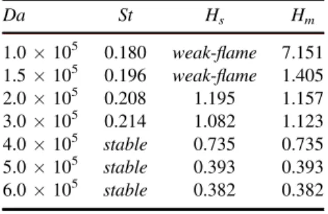
Table 1.Strouhal number, lift-off height(Hs) computed by the SFD technique, and average lift-off height(Hm) computed by DNS, for several values of the Damköhler number. Da St Hs Hm 1.0×10⁵ 0.180 weak-flame 7.151 1.5×10⁵ 0.196 weak-flame 1.405 2.0×10⁵ 0.208 1.195 1.157 3.0×10⁵ 0.214 1.082 1.123 4.0×10⁵ stable 0.735 0.735 5.0×10⁵ stable 0.393 0.393 6.0×10⁵ stable 0.382 0.382
and heat release rate and represent often not sustainableflame configurations, being strongly unstable.
Figure4 shows the temperaturefield and the heat release rate field computed by SFD: one can notice that the flame structure is completely different with respect to that computed by the DNS and shown infigure1.
3.4. Global stability: weak flame cases
Firstly, two weakflame cases will be analyzed, obtained for Da=105and 1.5×10⁵. In the related spectra, shown in figure5, among the modes that are well-converged, wefind four isolated unstable modes for each value of Da.
These results explain the strong unstable nature of weak flames. The eigenvalues obtained for these two cases are listed in table 2. One can notice that in this regime the Damköhler number does not strongly affect the eigenvalue growth rates and frequencies. For both values of Da, the fourth eigenvalue has a frequency close to theλi,DNScalculated from the DNS. Concerning the associated eigenvectors, they all have a similar shape as shown in figures6and7. The real components of these eigenvectors reveal that the instability zone is in the diffusive part of theflame, which is typical of weak flame cases (in agreement with Bucci et al (2016)) with a strong diffusion of production rate and radial development of the eigenmodes’ shape.
Figure 3. Base flow of cellular jet flame: non-dimensional temperature field in the longitudinal section(a) and in the crosswise section at x=1.3 (b) for Da=2.0×10⁵. Same temperature scale asfigure1.
Figure 4.Baseflow of cellular jet flame: temperature field (a) and ln(ω) field (b) for the weak-flame condition at Da=1.5×10⁵. Same temperature scale asfigure1.
Figure 5.The least-stable part of the global eigenvalue spectra for the weakflame cases at Da=105(circles) and Da=1.5×10⁵(crosses).
Table 2.Frequency and growth rate of the unstable eigenvalues at Da=105 and Da=1.5×10⁵
compared to frequencies obtained from Fourier transform of the lift-off height displacement signals.
Da=105 λ
i,DNS Da=1.5×10⁵ λi,DNS 0.141+0.734i 0.139+0.732i
0.065+0.824i 0.066+0.817i 0.051+0.630i 0.039+0.646i 0.014+0.953i 1.13 0.017+0.964i 1.23
3.5. Global stability: cellular flame cases
Figure8(a) shows the eigenvalue spectra for Da=2×10⁵, Da=3×10⁵and Da=4×10⁵. Varying the Damköhler number in this range, a transition between unstable and stableflame was found. In fact, for Da=4×10⁵all modes drop under the stability limit, confirming the results of the DNS. Amongst the modes that are well-converged, we find an isolated low-frequency unstable mode (mode A), and a set of stable convective high-frequency modes: these modes correspond to shear vortical structures and only the most unstable of these will be shown in detail(mode B). Mode A has lower frequency than mode B; moreover, the frequencies of both modes increase with Da, the vortical shape of the modes being almost unchanged. It is worth to notice that the modes here labeled as A and B have not a direct correspondence with the modes found by Nichols and Schmid(2008), since the test case considered in the present work is quite different from that used by Nichols and Schmid(2008) both for the chemical and fluid para-meters, so that a direct comparison of the results is not possible.
Table3provides the eigenvalues for each Damköhler number. A good matching is found between Im(λ) of mode A and λi,DNS: this indicates that the sampling employed in the algorithm is correct and validates our approach.
Figure 6. Isosurfaces of the non-dimensional temperature T (a) and of the mixture fraction Z(b) for the real component of the most unstable weak-flame global mode at Da=1.5×10⁵. Negative(blue) and positive (red) surfaces are shown.
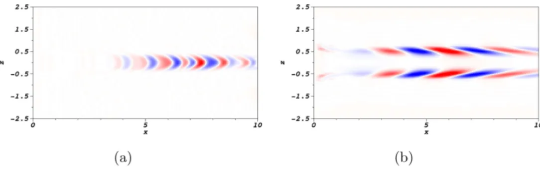
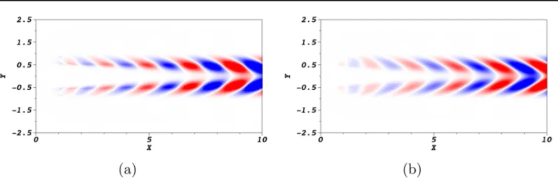
Figure 7. Contours of the non-dimensional temperature T (a) and of the mixture fraction Z(b) in a longitudinal plane for the real component of the most unstable weak-flame global mode at Da=1.5×10⁵
. Negative(blue) and positive (red) contours are shown.
Figure 8(b) shows the eigenspectra of the stable cases; the previously shown unstable modes, such as mode A, have negative growth rate despite their imaginary part remains about the same. Stable behavior is coherent with DNSs, in which the residual reduces in time in absence of SFD. On the other hand, modes B have higher frequency when increasing the Damköhler number.
Concerning the shape of the eigenvectors, small modifications are observed varying the Damköhler number; therefore, only those corresponding to Da=6×10⁵are provided. For thefirst of these modes, labeled mode A, real components, shown in figures9and10, indicate that the mode shape is dominant in the premixing zone between the inlet and theflame base. Thus, mode A appears to correspond to the pocket of instability upstream of theflame base. Temperature distribution shows two zones marked by different wave lengths: the front part, where the maximum amplitudes of the eigenmode are located, is characterized by oscillations having smaller wave length; whereas, the downstream oscillations, similar to the Kelvin– Helmholtz vortices observed by DNS, are characterized by a higher wave length.
However, even if both instability mechanisms are involved for mode A, the effect of the wavemaker in the premixing zone is dominant. Figure9shows that the present global stability analysis allows one to predict the three-dimensional structure of these modes, which are char-acterized by different azimuthal wave numbers along the axis of theflame. In fact, it appears that, for mode A, the azimuthal wave number tends to zero towards the tip of theflame. These figures also show that the axial wavenumber is varying along the streamwise direction. Moreover, both figures9and10show the presence of an instability front in the premixed region aligned with the lean branch of the tripleflame. Finally, figures11(a) and (b) provide the temperature distribution
Figure 8. Global eigenvalue spectra for cellular flames at (a) Da=2×10⁵, Da=3×10⁵ and Da=4×10⁵; (b) Da=4×10⁵, Da=5×10⁵ and Da=6×10⁵. Filled symbols represent modes A and B.
Table 3. Frequency and growth rate of the unstable eigenvalues at Da=2×10⁵, Da=3×10⁵, and Da=4×10⁵ compared to frequencies obtained from Fourier transform of the lift-off height displacement signals.
Da=2×10⁵ Da=3×10⁵ Da=4×10⁵ Mode A +0.159+1.183i +0.179+1.247i −0.077+1.531i Mode B −0.211+2.070i −0.212+2.213i −0.359+2.414i λi,DNS 1.306 1.344
for mode A at two cross section corresponding to x= 4.5 and x = 8.0, respectively. The contours clearly show again the 4-cell structure of the eigenmode.
The second mode, labeled mode B, provided infigure12, is located further downstream along the diffusive part of the flame; it is clearly a Kelvin–Helmholtz mode, which grows both in the radial and axial direction(convective instability).
Also the corresponding contours of temperature and mixture fraction are located along the diffusive zone of theflame, as shown in figure13. It is noteworthy that this mode is active in the flame region as mode B described by Qadri et al (2015); however, its frequency is higher than that of mode A, whereas, in the test case considered by Qadri et al(2015), mode B had a lower frequency with respect to mode A. This different behavior could be due to the different parameters of the combustion model and to three-dimensional effects.
4. Conclusions and future developments
In this work, a numerical method based on the time-stepper approach proposed by Edwards et al(1994) and Bagheri et al (2009) has been combined with a numerical linearization of the
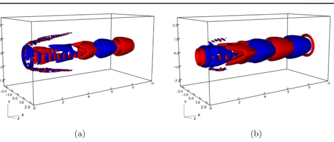
Figure 9. Isosurfaces of the non-dimensional temperature T (a) and of the mixture fraction Z(b) for the real component of mode A at Da=6.0×10⁵. Negative(blue) and positive(red) surfaces are shown.
Figure 10. Contours of the non-dimensional temperature T (a) and of the mixture fraction Z (b) in a longitudinal plane for the real component of mode A at Da=6.0×10⁵. Negative(blue) and positive (red) contours are shown.
governing equations and employed to study the global stability of three-dimensional reacting flows. This method allows one to analyze the stability of diffusion flames without the direct evaluation and storage of the linearized operator; in this way, a remarkable reduction of the storage capacity is achieved, which renders the method suitable for three dimensional flow computations and complex combustion models. Furthermore, the employed numerical approach, avoiding the analytical evaluation of the Jacobian matrices, represents a very flexible approach, which can be applied straightforwardly to any complex system of con-servation equations governing the dynamics of a reactingflow provided that a DNS solver is available. The present work provides thefirst application of the global stability analysis to a
Figure 11.Non-dimensional temperature distribution in the cross sections at x= 4.5 (a) and x= 8.0 (b) for the real component of mode A at Da=6.0×10⁵. Negative(blue) and positive(red) contours are shown.
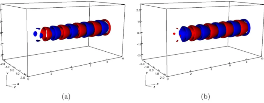
Figure 12. Isosurfaces of the non-dimensional temperature T(a) and of the mixture fraction Z for the real component of mode B at Da=6.0×10⁵
. Negative(blue) and positive(red) surfaces are shown.
three-dimensional reactingflow. The results obtained in the present work demonstrate that the proposed approach is useful to identify the main mechanisms of instability with a reasonable computational cost.
The method was validated versus the results of Qadri et al(2015) using the same test case proposed by Nichols and Schmid (2008) concerning an axisymmetric jet diffusion flame (Mancini et al 2017).
In the present work, the numerical model has been employed to study the stability of a three-dimensional jet diffusionflame with cellular structure. The baseline case was the same employed by Lo Jacono et al (2003), providing the experimental observation of cell structures in reactiveflows using the EPFL jet flame facility, and by Frouzakis et al (2005), who have performed numerical simulations and a local stability analysis. Since the focus of the present paper is the stability analysis, a simple mixture fraction combustion model has been employed. Despite the mixture fraction model does not consider transport equations for species concentrations, we obtained a cellular structure for all considered Damköhler numbers and theflame behavior in terms of lift-off height is coherent with the experimental results.
Thanks to the global stability analysis it was possible to study the three-dimensional eigenmode shape related to the most representative eigenvalues in the range 105Da6×105. Two different families of modes have been identified: we labeled as mode A the low-frequency most unstable mode that contains instabilities related to the premixing zone of the flame and presents higher frequency peaks in that zone; whereas, the high-frequency mode was labeled mode B, which is the most representative of the instabilities in the diffusive rear region of the flame (associated with Kelvin–Helmholtz vortices). Moreover, unlike previous two-dimensional analyses, the present three-dimen-sional stability analysis has been able to compute for the first time non-axisymmetric modes, which are responsible for the cellular structure of the flame. Thus, the main contribution of this paper has been to provide a physical explanation for the onset of a cellular structure of theflame, linking it to a Hopf bifurcation arising for decreasing values of the Damköhler number.
Future development of this work could be to employ a more accurate chemical reaction model that would allow one to consider different Lewis numbers and to have a better matching with real experimental assumptions.
Figure 13. Contours of the non-dimensional temperature T (a) and of the mixture fraction Z(b) for the real component of mode B at Da=6.0×10⁵. Negative(blue) and positive(red) contours are shown.
Acknowledgments
This work was granted access to HPC resources of IDRIS under allocation x20162a6362 made by GENCI(Grand Equipement National de Calcul Intensif). The authors also wish to acknowledge the computational resources of the PrInCE project (grant PONa3-00372-CUP D91D11000100007) at Politecnico di Bari. M A Bucci is also acknowledged for fruitful discussions.
Appendix
In this section, details about the numerical method used for evaluating the Jacobian matrix, as well as a validation of the grid, are provided. The numerical evaluation of the Jacobian matrix for stability analysis is a well established technique employed by several authors (Mack et al2008, Mack and Schmid2010). The present work provides the first application of such a technique for the global stability analysis of three-dimensional reactingflows. For applying this method, one should first ensure that the value of ò in equation (14) is small enough to accurately approximate (with a nonlinear operator) the linear evolution of the perturbations. However, even if the initial value ofò is very small, the flow might be prone to strong energy growth due to modal or nonmodal mechanisms, as in some of the cases considered in this work. In these cases, a renormalization of the amplitude of the pertur-bation during the time integration is necessary in order to ensure that theflow remains in the linear regime during the whole time integration. This method guarantees a good approx-imation of the eigenvalues even when theflow is highly unstable. In this work, for all of the considered cases, we have applied such a renormalization everyΔt (namely, every time a snapshot is extracted from the DNS for creating the Krylov subspace in the Arnoldi method), rescaling the initial condition for obtaining the following snapshot such that its L2 norm is equal toò. Concerning the value of ò, we have chosen to employ ò=10−7, which is a reference value employed in the literature (see, for instance, the work of Gibson et al (2008)). Furthermore, using the two-dimensional flow case of Qadri et al (2015) as a test case, we have verified that the leading eigenvalues change less than 1% when using ò=10−8.
Concerning the discretization, all computations have been performed using a Cartesian grid. Inside each cell, the nodes are distributed according to the spectral-element discretization based on Legendre polynomials. To choose the order of the Legendre polynomial employed in the study, we have used different values of N for the case with Da=6×10⁵. The eigenspectrum as well as the eigenvector shapes obtained for N=8 and N=9 are very similar. Figure A1 provides the eigenvalue spectrum obtained with N=8 and N=9, showing a satisfactory convergence level, whereas the non-dimensional temperature distributions in the cross sections at x= 4.5 (a) and x = 8.0 (b) for the real component of mode A, are provided in figureA2. One can compare these results with those provided in figure11 (obtained with N=8), noticing that the 4-cell structure of the mode does not change with the order of the polynomial reconstruction. Thus, for all the computations provided in this work, a polynomial order N=8 has been used.
ORCID iDs
P De Palma https://orcid.org/0000-0002-7831-6115
References
Åkervik E, Brandt L, Henningson D S, Hœpffner J, Marxen O and Schlatter P 2006 Phys. Fluids18 068102
Bagheri S,Åkervik E, Brandt L and Henningson D S 2009 AIAA J.47 1057–68 Bucci M A, Robinet J C and Chibbaro S 2016 Combust. Flame167 132–48
Edwards W S, Tuckerman L S, Friesner R A and Sorension D C 1994 J. Comput. Phys.110 82–102 Fischer P, Lottes J and Kerkemeir S 2008‘nek5000 Web pages’http://nek5000.mcs.anl.gov Frouzakis C E, Tomboulides A G, Papas P, Fischer P F, Rais R M, Monkewitz P A and Boulouchos K
2005 Proc. Combust. Inst.30 185–92
Figure A1.Eigenvalue spectrum for Da=6×10⁵obtained with N=8 and N=9.
Figure A2.Non-dimensional temperature distributions in the cross sections at x=4.5 (a) and x=8.0 (b) for the real component of mode A obtained for Da=6×10⁵
Gibson J F, Halcrow J and Cvitanović P 2008 J. Fluid Mech.611 107–30
Gorman M, El-Hamdi M, Pearson B and Robbins K A 1996 Phys. Rev. Lett.76 228
Gunaratne G H, El-Hamdi M, Gorman M and Robbins K A 1996 Mod. Phys. Lett. B10 1379–87 Loiseau J C, Robinet J C, Cherubini S and Leriche E 2014 J. Fluid Mech.760 175–211
Lo Jacono D, Papas P and Monkewitz P A 2003 Combust. Theory Modelling7 635–44 Mack C J and Schmid P J 2010 J. Comput. Phys.229 541–60
Mack C J, Schmid P J and Sesterhenn J L 2008 J. Fluid Mech.611 205–14
Mancini C, Farano M, De Palma P, Robinet J C and Cherubini S 2017 Energy Proc.126 867–74 Michalke A 1984 Prog. Aerosp. Sci.21 159–99
Nichols J and Schmid P J 2008 J. Fluid Mech.609 275–84
Peters N 2000 Turbulent Combustion(Cambridge: Cambridge University Press) Qadri U A, Chandler G J and Juniper M P 2015 J. Fluid Mech.775 201–22 Tomboulides A G, Lee J C Y and Orszag S A 1997 J. Sci. Comput.12 139–67