Variabilité des communautés benthiques à différentes échelles
spatiales et dans différents habitats
Mémoire présenté
dans le cadre du programme de maîtrise en océanographie en vue de l'obtention du grade de maître ès sciences
PAR
© CAMILLE ROBINEAU
Avertissement
La diffusion de ce mémoire ou de cette thèse se fait dans le respect des droits de son auteur, qui a signé le formulaire « Autorisation de reproduire et de diffuser un rapport, un mémoire ou une thèse ». En signant ce formulaire, l’auteur concède à l’Université du Québec à Rimouski une licence non exclusive d’utilisation et de publication de la totalité ou d’une partie importante de son travail de recherche pour des fins pédagogiques et non commerciales. Plus précisément, l’auteur autorise l’Université du Québec à Rimouski à reproduire, diffuser, prêter, distribuer ou vendre des copies de son travail de recherche à des fins non commerciales sur quelque support que ce soit, y compris l’Internet. Cette licence et cette autorisation n’entraînent pas une renonciation de la part de l’auteur à ses droits moraux ni à ses droits de propriété intellectuelle. Sauf entente contraire, l’auteur conserve la liberté de diffuser et de commercialiser ou non ce travail dont il possède un exemplaire.
Jean-Claude Brêthes, président du jury, UQAR ISMER Philippe Archambault, directeur de recherche, UQAR ISMER Bruno Vincent, codirecteur de recherche, UQAR
Chris McKindsey, codirecteur de recherche, IML Frédéric Guichard, examinateur externe, Mc GILL
REMERCIEMENTS
Je tiens, tout d'abord, à remerCIer particulièrement mon directeur Philippe Archambault, pour ses conseils et son soutien. Je remercie aussi Bruno Vincent pour les données qu'il m'a fournies, ainsi que pour son aide tout au long de ce projet.
Je voudrais également remercier Hannah Cubaynes qui m'a aidée et soutenue, que ce soit sur le terrain ou au laboratoire. Je remercie aussi Timothée Govare et Quentin Cyr, sans qui le terrain n'aurait pas été réalisable et aussi agréable. Merci aussi à toutes les personnes travaillant au laboratoire d'écologie benthique, pour leur aide et leur présence.
Je remercie aussi Sylvie Brulotte pour m'avoir permis d'utiliser une partie de ses données et pour son aide quant à l'interprétation des résultats.
Merci à ma famille et mes amis pour m'avoir soutenue et encouragée jusqu'au dernier moment.
Et je voudrais rajouter des remerciements pour une aide inespérée alors que je me trouvais à l'autre bout du monde. Merci à Cyril Gallut et Nadia Ameziane qui m'ont donné de leur temps afin de me permettre de finaliser ce mémoire. Merci à tous mes cohivernants de la T A61 pour leur soutien moral et à Benoît qui m'a supportée tous les jours et m'a forcée à prendre des décisions.
RÉSUMÉ
La connaissance de la variabilité spatiale des communautés benthiques est un outil utile au développement de théories générales et à l'établissement de plans de conservation des écosystèmes, une perturbation sporadique pouvant causer une augmentation de la variabilité spatiale. Cette connaissance est obtenue notamment par l'utilisation de plans d'échantillonnage hiérarchique, afin de déterminer l'échelle de plus grande variabilité. Elle correspond à l'échelle à laquelle les processus majeurs jouent un rôle important. Ce type d'échantillonnage a été utilisé afin de comparer la variabilité de la biodiversité et de l'environnement associé, dans trois habitats différènts (deux intertidaux et un profond "" 300 m) de l'estuaire du Saint-Laurent (Québec, Canada). La variabilité spatiale de la mye, Mya arenaria a été estimée avec le même type d'échantillonnage au niveau de deux gisements de la Haute-Côte-Nord (Québec, Canada). En complément, l'étude de la population de la mye, espèce pêchée commercialement au niveau des gisements de la Haute-Côte-Nord, a été utilisée pour tester si sa variabilité spatiale avait été affectée sur une période de quarante ans. Des données d'échantillonnage systématique de pas de 50 mètres, datant de 1967-69 et de 2002-09, ont servi à la comparaison. L'échelle de plus grande variabilité est dépendante de la communauté étudiée mais aussi de l'espèce~ avec une plus grande variabilité de la communa,uté à l'échelle du centimètre pour le milieu profond et à l'échelle de 200 mètres et du kilomètre pour les milieux intertidaux. La variabilité de la granulométrie du sédiment réagit de manière similaire à celles des données de densité de l'assemblage. Les résultats varient aussi suivant l'indice choisi. La variabilité spatiale de la mye n'a pas été affectée pendant la période étudiée. Sa population, par contre, a montré un décalement du maximum de densité vers des tailles plus petites et aussi un déplacement vers des zones à temps d'émersion plus court. Mais dépendamment du gisement, les réponses étaient variables malgré ces tendances. Cette étude montre l'importance d'effectuer de plus amples projets sur la question de la variabilité spatiale, au vu de la diversité des réponses en fonction de l'environnement et des espèces. Il est très difficile de prédire, en l'état actuel, quelle sera l'échelle de plus grande variabilité d'un système, ainsi que sa réaction face à une perturbation.
Mots clés: variabilité spatiale, biodiversité benthique, échelle spatiale, échant~llonnage hiérarchique, Mya arenaria, pêche, évolution des gisements.
ABSTRACT
The knowledge of benthic communities' spatial variability is a useful too1 in general theories development and in conservation plan establishment, a pulse perturbation causing an increase in the spatial variability. To determine the spatial sc ale of major variability, corresponding to the scale at which major processes occur, nested sampling designs are useful tool. This kind of design has been used to compare the biodiversity and the environ mental variabilities in three different habitats (two intertidals and one deep "" 300 m) in the St. Lawrence estuary (Québec, Canada) and also to study the spatial variability of the clam, Mya arenaria. Furthermore the clam population, species being commercially fished in the beds of the Upper North Shore (Québec, Canada), has been used in order to test if its spatial variability had been affected by fishing for a fort y years period. Data from systematic sampling designs of 50 m step, from 1967-69 to 2002 and 2009 were compared. The scale of largest variability was dependent on the community under study and also varied between species, with a largest variability of the community at the centimeter scale for the deep habitat and at the 200 meters scale and kilometer scale respectively for the intertidal habitats. Grain size variability reacted in the same way as density community variability. Chosen indices affected also the obtained results. Clam spatial variability was not affected during studied period. However, clam population showed a move of the peak of density per size class towards smaller sizes and also a move of the population distribution towards area with shorter emersion time. Despite sorne trends, responses were variable depending on the beds. This study shows the importance to realize more projects on this subject, considering the response diversity depending on the environ ment and the species. It is very difficult at that point to predict what the spatial scale of largest variability would be and thus to predict its reaction to a perturbation.
. Keywords: spatial variability, benthic biodiversity, spatial scale, hierarchical sampling, Mya arenaria, fishing, beds evolution.
TABLE DES MATIÈRES
REMERCIEMENTS ... vii
RÉSUMÉ ... ix
ABSTRACT ... xi
TABLE DES MATIÈRES ... xiii
LISTE DES TABLEAUX ... xv
LISTE DES FIGURES ... xix
INTRODUCTION GÉNÉRALE ... 1
CHAPITRE 1: VARIABILITE SPATIALE DE LA BIODIVERSITE BENTHIQUE A DIFFERENTES ECHELLES SPATIALES ET DANS DIFFERENTS HABITATS ... 5
1 .1 Résumé ... ~ ... 5
1.2 Introduction ... 6
1.3 Material and Methods ... 9
1.4 Results ... 15
1 .5 Discussion ... 25
1.6 Conclusion ... 28
CHAPITRE 2 EVOLUTION DE LA POPULATION DE LA MYE (Mya arenaria) ET DE SA VARIABILITE SPATIALE ENTRE 1967 ET 2009 DANS L'ESTUAIRE DU SAINT-LAURENT ... 31 2.1 Résumé ... 31 2.2 Introduction ... 32 2.3 Matériel et Méthodes ... 35 2.4 Résultats ... 45 2.5 Discussion ... 57
2.6 Conclusion ... 62 CONCLUSION GÉNÉRALE ... 65 RÉFÉRENCES BIBLIOGRAPHIQUES ... 69 Annexe 1 : Carte des zones avec les densités les plus forte (la densité totale et la
densité de myes de taille commerciale), pour la baie Blanche, le cap Colombier, le
havre Colombier et les îlets à Jérémie ... 81 Annexe 2 : Cartes des abondances de myes (totale et de taille commerciale) et des caractéristiques du sédiment (MO, Vase), pour la baie Blanche, le Cap Colombier, le Havre Colombier et les Îlets à Jérémie, pour 1968 et 2009 ... 87
Annexe 3 : Cartes des stations pour la baie Blanche, le cap Colombier, le havre Colombier et les îlets à Jérémie, pour 1968 et 2009 ... 93
LISTE DES TABLEAUX
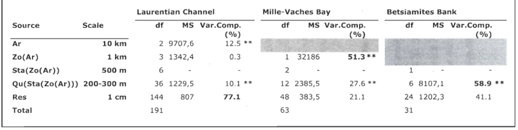
Table 1: Hierarchical PERMANOV A for differences in organisms density assemblage data (Bray-Curtis matrix) in the Laurentian Channel, the Mille-Vaches Bay and Betsiamites Bank at the different spatial scales. Estimates of variance component (%) are included. **: significant «0.001). bold
=
spatial scale participating the most to the total variability. grey=
inexistent spatial scale. " - "=
pooled scale due to negative value. Ar=
Area, Zo=
Zone, Sta=
Station, Qu=
Quadrat, Res=
Residuals, Var.comp=
Variance component, df = degree of freedom, MS = mean square ... 18 Table 2: Variance component (%) of diversity indices (Bray-Curtis matrix:Shannon-Wiener index, species richness, total density) compute after hierarchical PERMANOVA, for the Laurentian Channel (LC), the Mille-Vaches Bay (MVB) and Betsiamites Bank (BET) at the different spatial scales. grey = inexistent spatial scale. bold
=
spatial scale participating the most to the total variability. " - "=
pooled scale due to negative value. Var.comp=
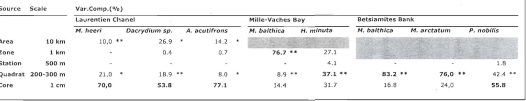
Variance component. ... 19 Table 3: Hierarchical PERMANOV A (Bray-Curtis matrix) for differences in the most abundant species in the Laurentian Channel (M. heeri, Dacrydium sp., A. acutifrons), the Mille-Vaches Bay (M. balthica, H. minuta) and Betsiamites Bank (M. balthica, M. arctatum, P. nobilis). *: significant «0.05); **: significant «0.001). bold=
spatial scale participating the most to the total variability. grey=
inexistent spatial scale. " - "=
pooled scale due to negative value. Var.comp=
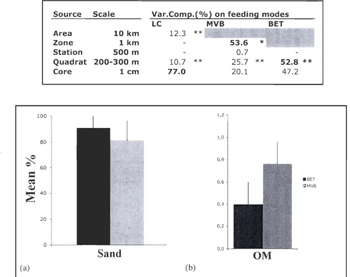
Variance component. ... 22 Table 4: Variance component (%) for feeding mode assemblage data (Bray-Curtis matrix), compute after a hierarchical PERMANOV A, in the Laurentian Channel (LC), the Mille-Vaches Bay (MVB) and Betsiamites (BET). *: significant «0.05); **: significant «0.001). bold=
spatial sc ale participating the most to the total variability. grey=
inexistent spatial scale. " - "=
pooled scale due to negative value. Var.comp=
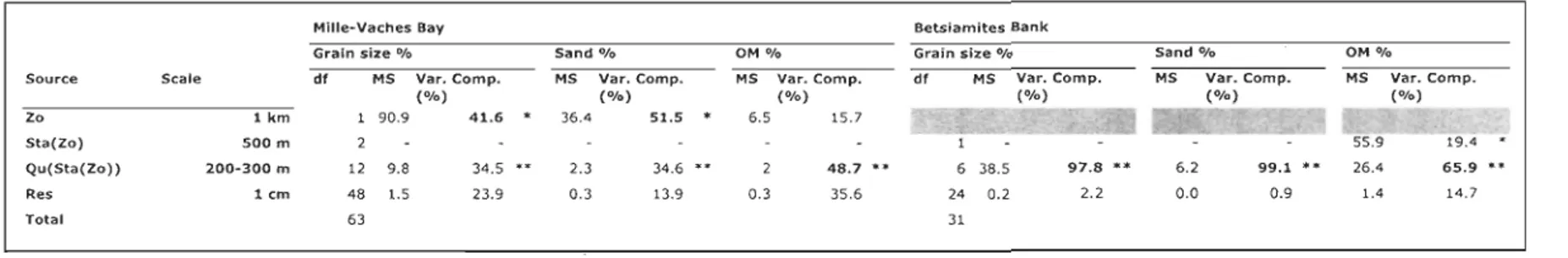
Variance component. ... 23Table 5: Hierarchical PERMANOV A for differences in the sediment characteristics (grain size, sand %, organic matter (OM%» data (euclidean matrix) for Mille-Vaches Bay and Betsiamites Bank. *: significant «0.05); **: sig"nificant «0.001). bold
=
spatial sc ale participating the most to the total variability. " - "=
pooled scale due to negative value. Zo=
Zone; Sta=
Station; Qu=
Quadrat; Res=
Residuals. Var.comp=
Variance component, df=
degree of freedom, MS=
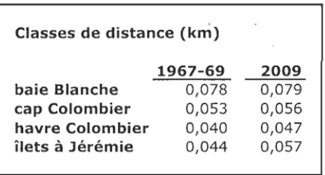
mean square ... 24 Tableau 6 : Valeurs des classes de distance (km) utilisées pour les semi-variogrammes et la corrélation de Dutilleul ... .44 Tableau 7 : PERMANOVA hiérarchique sur la granulométrie, sable/vase % et la MO% (matrice euclidienne, 9999 permutations) pour la baie des Mille-Vaches et le banc de Betsiamites. Les valeurs des composantes de la variance sont incluses.*
:
significatif (p<0,05) ; ** : significatif (p<O,OOl). Gras = échelle spatiale participant le plus à la variabilité totale. Gris=
échelle spatiale inexistante. " - "=
échelle groupée à cause de valeurs négatives. Zo=
Zone, Sta=
Station, Qu=
Quadrat, Res=
Résidus, dl=
degrés de liberté, SC=
somme des carrés, Comp.Var.=
composant de la variance ... .47 Tableau 8 : PERMANOV A hiérarchique sur les classes de taille de mye, les myesnon-commerciales et les myes commerciales (matrice de Bray-Curtis), 9999 permutations.Valeurs des composantes de la variance sont incluses.
** : significatif
(p<O,OOl),* : significatif (p<0,05).
Gras=
échelle spatiale participant le plus à la variabilité totale. Gris=
échelle spatiale inexistante. " - "=
échelle groupée à cause de valeurs négatives. Zo=
Zone, Sta=
Station, Qu=
Quadrat, Res=
Résidus, dl=
degrés de liberté, SC=
somme des carrés, Comp.Var.=
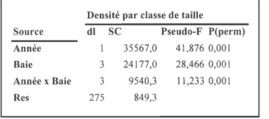
composant de la variance ... .49 Tableau 9: PERMANOVA croisée sur la densité par classe de taille de M. arenaria (matrice de Bray-Curtis, 9999 permutations). dl=
degrés de liberté, SC=
somme des carrés, P(perm)=
probabilité calculée par permutation ... 52 Tableau 10 : Probabilités associées de Dutilleul (1993) aux coefficients de Pearson entre le pourcentage de sable et les variables biologiques (densité totale et myes de taillecommerciale) pour la baie Blanche (BB), le cap Colombier (CC), le havre Colombier (HC) et les Hets à Jérémie (U). Gras = valeurs significatives a = 0,05 ... 57
LISTE DES FIGURES
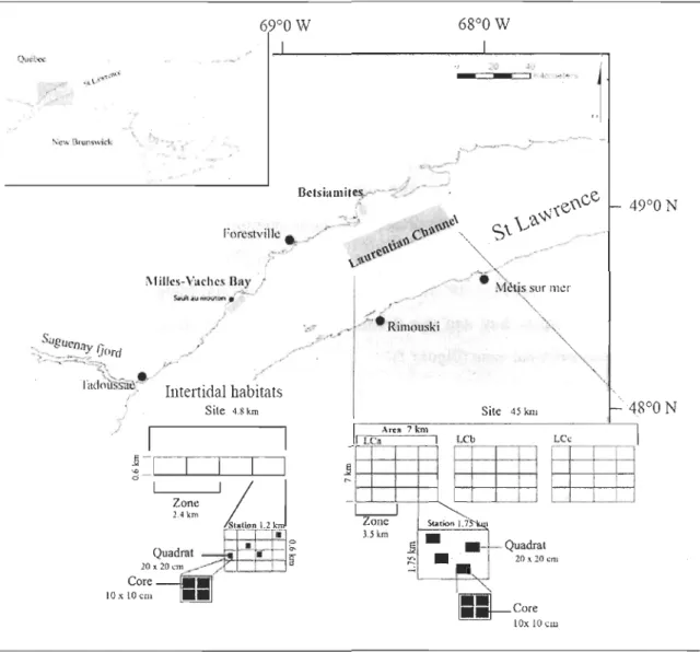
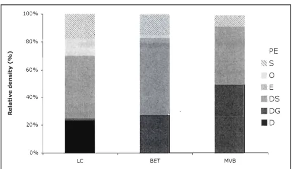
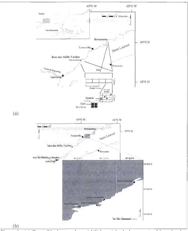
Figure 1: St. Lawrence estuary (Québec, Canada) showing the study sites. Expanded section shows t~e position of the two intertidal habitats (Mille-Vaches Bay and Betsiamites) and the deep habitat (Lauren tian channel) and their respective sampling design. Grey area: sampling area ... 10 Figure 2: Relative density (%) of the different feeding modes, for the Laurentian Channel (Le), the Mille-Vaches Bay (MVB) and Betsiamites Bank (BET). D
=
deposit feeder, DG = deposit feeder + grazer, DS = deposit feeder + suspension feeder, E = detritivore,O = omnivore, S = suspension feeder, PE = predator + detritivore ... 16 Figure 3: Mean percentage (+ SD) of sediment characteristics, (a) Sand % and (b) Organic Matter (OM)%, for Mille-Vaches Bay (MVB) and Betsiamites Bank (BET) ... 23 Figure 4: (a), Zone d'étude pour la variabilité spatiale de la mye et schéma du plan d'échantillonnage hiérarchique utilisé dans la baie des Mille-Vaches et le banc de Betsiamites. (b) Zone d'étude de l'évolution des gisements de myes (baie du Moulin à Baudes, baie Blanche, cap Colombier, havre Colombier et îlets à Jérémie) entre 1967-69 et 2002-09 ... ~ ... 37 Figure 5: Valeurs moyennes (+ erreur type) des caractéristiques du sédiment, (a) pourcentage en sable, (b) pourcentage de MO, pour la baie des Mille-Vaches (BMV, gris) et le banc de Betsiamites (BET, noir) ... 48 Figure 6: (a) Densité moyenne par baie (+ erreur type) de myes, pour le banc de Betsiamites (BET) et la baie des Mille-Vaches (BMV) et (b) densité moyenne de myes de taille commerciale et de taille non-commerciale pour le banc de Betsiamites (+ erreur type) ... 48Figure 7 : (a) Densité totale, (b) densité
qe
myes de taille non commerciale et (c) densité de mye de taille commerciale (+ erreur type) de M. arenaria, pour le cap Colombier (CC), le havre Colombier (HC), les Hets à Jérémie (Il) et la baie Blanche (BB) et par année, 1969 (gris) et 2009 (noir). Résultats des tests deux à deux de la PERMANOVA (matrice euclidienne, 9999 permutations), ligne divisée: différence significative (p<0.05), ligne continue: différence non significative (p>Ü.05) ... 53 Figure 8 : Densité de myes en fréquence par classe de taille de 1 cm, par baie (a) baie Blanche, (b) havre Colombier, (c) cap Colombier, (d) îlets à Jérémie et (e) Moulin àBaudes et par année: 1967-69 (gris), 2002~09 (noir) ... 54 Figure 9 : Semi-Variogramme sur la densité totale de myes par carotte pour (a) la baie Blanche (BB), (b) le cap Colombier (CC), (c) le havre Colombier (HC) et (d) les îlets
à Jérémie (IJ) ... : ... 56
Figure 10 : Moyenne (+ erreur type) du (a) pourcentage de MO (matière organique) et du (b) pourcentage de vase, en 2009 pour la baie Blanche (BB), le cap Colombier (CC), le havre Colombier (HC) et les îlets à Jérémie (Il) , ... 56
INTRODUCTION GÉNÉRALE
L'ensemble de ce mémoire s'attache à travailler sur un point soulevé notamment par Chapman et Tolhurst (2Q07) : aucune étude en milieu marin n'a examiné la variabilité à
travers plusieurs types de faunes et de propriétés physiques et biologiques, ni n'a essayé de faire des comparaisons à travers plus d'un habitat. En choisissant des habitats différents et des conditions anthropiques différentes pour la présente étude, nous essayons d'y apporter
un début de réponse.
L'espace est une notion importante en écologie, mais difficile à appréhender. En effet, il est difficile d'avoir une vision globale des écosystèmes, surtout dans le milieu
benthique marin. L'espace doit être défini précisément afin de permettre une répétitivité des mesures et une compréhension adéquate du système. D'autant plus si l'on se place dans un
contexte où l'on cherche à développer des théories générales et à répondre' aux besoins des problématiques liées à la conservation (Allen et Hoekstra, 1991 ; Levin, 1992; Underwood et Petraitis, 1993 ; Armonies, 2000 ; Kaiser et al., 2001 ; Benedetti-Cecchi, 2003).
Au niveau de l'étude des communautés et des patrons de répartition des organismes,
un problème se pose avec l'échelle spatiale à laquelle s'effectue cette étude. L'échelle
spatiale n'est pas une propriété de la nature, elle est associée à notre manière de voir (Allen et Starr, 1982). Nous avons besoin de définir cette échelle précisément afin de pouvoir comparer les conclusions de différentes études entre elles. En effet, les processus écologiques, tels que la compétition ou les relations prédateur proie, agissant sur la répartition des organismes ne sont pas identiques à toutes les échelles. Par exemple, un prédateur aura pour effet d'homogénéiser l'abondance de sa proie à grande échelle. À une échelle locale, celui-ci se concentrera en agrégats sur sa proie, ce qui fragmentera la répartition spatiale de celle-ci. Les processus écologiques identifiés à une échelle ne sont pas non plus nécessairement la somme des processus écologiques présents à une échelle plus fine (Turner et al., 1989; Bunnell et Huggart, 1999; Bishop et al., 2002 ; Underwood
et Chapman, 1998). De plus, nous ne pouvons pas être sûr que ce que nous comprenons à une échelle dans un habitat donné soit applicable dans tous les habitats (Barry et Dayton, 1991) .
Ces processus écologiques découlent de facteurs abiotiques et biotiques qUI interagissent avec les organismes vivants (ex: les caractéristiques du sédiment, le taux de mortalité ... ). Ces facteurs et leurs interactions sont aussi dépendants de l'échelle spatiale à laquelle on les étudie (Meentemeyer et Box, 1987). De ce point découle des variabilités spatiales de la densité et de la diversité des organismes différentes selon les échelles étudiées (Fraschetti et al., 2005). De plus, la multiplicité des, interactions entre facteurs abiotiques et biotiques suscite un phénomène de regroupement des individus en agrégats. Ceux-ci peuvent être de taille variable et sont en général le reflet de l'échelle à laquelle les processus écologiques s'expriment (Underwood et Chapman, 1996). Les agrégats peuvent aussi s'imbriquer les uns dans les autres d'où l'importance de déterminer l'échelle à laquelle le processus, que l'on cherche à étudier, s'effectue (Underwood et Chapman, 1996). La présence et l'importance, selon les habitats et les échelles spatiales, de chacun des facteurs ne sont malheureusement peu ou pas connues. Il est de ce fait important d'essayer de définir et de comprendre les influences de chacun des facteurs, dans le plus grand nombre d'habitats et d'échelles spatiales (Meentemeyer et Box, 1987; Thrush et al.,
1996; Ellis et al., 2000; Zajac et al., 2000; Whittaker et al., 2001 ; Cushman et McGarigal, 2004; Thrush et al., 2005 ; Fujii, 2007; Reichert et al., 2008).
La variabilité de la densité des organismes est différente suivant les échelles spatiales. L'échelle à laquelle la variabilité de la densité des organi~mes est la plus forte est particulièrement intéressante. En effet, cette échelle correspondrait à l'échelle spatiale où les processus écologiques majeurs jouent un rôle clef dans la répartition des organismes (Underwood et Chapman 1998 ; Reichert, 2008 ; Chapman et Underwood, 2008 ; Chapman
et al., 2010). La connaissance de l'échelle pour laquelle la variabilité de la densité des
processus et sur d'éventuelles modifications de l'environnement jouant sur la répartition des organismes (U nderwood et Petraitis, 1993 ; Gray, 2000).
Dans ce mémoire nous abordons la problématique de la variabilité spatiale de la densité d'organismes marins benthiques de l'estuaire du Saint-Laurent (Québec, Canada) à deux niveaux différents. Dans une première partie en comparant trois habitats distincts puis dans une deuxième partie nous nous sommes concentrés sur les effets d'une perturbation sur une population donnée.
Dans la première partie nous comparons différentes échelles spatiales avec les variabilités les plus importantes de la biodiversité et du sédiment comme facteur abiotique, dans trois habitats benthiques. Deux habitats sont intertidaux avec des hydrodynamismes différents et le troisième est un habitat profond situé dans le chenal du Saint-Laurent. Dans ces trois habitats nous avons échantillonné à différentes échelles spatiales. Nous avons retenu le sédiment comme facteur abiotique pour sa représentativité des conditions environnementales extérieures et son importance pour les organismes benthiques (Gray, 1974; Snelgrove, 1997; Ramey et Snelgrove, 2003; Anderson, 2008). Par exemple, l'hydrodynamisme présent et les apports en matière organique peuvent être déduits de la granulométrie et du pourcentage de matière organique (Gray, 1981 ; Levin, 2001 ; Zajac, 2008).
Les résultats nous permettront de tirer des conclusions sur les facteurs importants pour la répartition des organismes, dans la région de l'estuaire du Saint-Laurent. La détermination des échelles où la variabilité des différents paramètres est la plus forte permettra aussi d'ajouter de nouvelles informations sur ce sujet déjà étudié par de nombreux auteurs (ex: Fraschetti et al., 2005 et les références à l'intérieur). Cela est, par contre, une des premières études sur le sujet portant sur plusieurs habitats avec les mêmes échelles spatiales prise en compte, ce qui nous permet de réaliser facilement des comparaisons.
Dans la seconde partie nous étudions les effets d'une perturbation ponctuelle (la pêche à pied) sur une population de mye, Mya arenaria Linnaeus, 1758, mollusque bivalve et sa variabilité spatiale. Il a été montré par plusieurs auteurs qu'une perturbation ponctuelle provoquait une augmentation dans la variabilité spatiale principalement au niveau de la communauté étudiée (Caswell et Cohen, 1991 ; Chapman et al., 1995 ; Cervin et al., 2004 ; Terlizzi .et al., 2005a, 2005b ; Séguin et Archambault, soumis). Cette observation pourrait alors être un diagnostic à l'apparition d'une perturbation dans une communauté déjà connue (Gray, 1997). Nous considérons que la pêche à pied de la mye est ponctuelle étant donnée qu'elle n'est autorisée que pendant le printemps et réalisée principalement pendant les périodes de grandes marées (MPO, 2008). Possédant des données antérieures à l'essor de la pêche à pied commerciale (1967-1969 ; Lavoie, 1969, 1970) et ayant eu la possibilité d'effectuer des prélèvements quarante ans plus tard, nous voulons comparer la répartition et la variabilité spatiale de la mye dans plusieurs baies de la zone intertidale sujettes à cette pêche. Cette étude permet d'avoir un aperçu des stocks et d'observer comment une espèce soumise à une pêche se comporte dans l'espace.
CHAPITRE 1 : VARIABILITE SPATIALE DE LA BIODIVERSITE
BENTHIQUE A DIFFERENTES ECHELLES SPATIALES ET DANS
DIFFERENTS HABIT A TS
1.1 RESUME
L'étude de la variabilité spatiale de la biodiversité benthique à travers les échelles spatiales est une problématique importante pour l'étude des processus écologiques. Le but de cette étude est de déterminer l'échelle spatiale de plus grande variabilité dans trois habitats différents (deux intertidaux et un profond
=
300 m) de l'estuaire du Saint-Laurent (Québec, Canada), et d'identifier la corrélation entre sédiment et biodiversité. Un plan d'échantillonnage hiérarchique est utilisé, allant du centimètre à la dizaine de kilomètres. La biodiversité est considérée en termes de richesse en espèce, indice de Shannon-Wiener, densité totale, biomasse totale et d'assemblage en données de densité, de biomasse et de modes alimentaires. Le sédiment est identifié par la granulométrie, le pourcentage de sable et le pourcentage de matière organique. Les échelles de plus grande variabilité spatiale sont différentes entre les différents indices. Pour les données d'assemblage, en milieu profond, l'échelle de plus grande variabilité correspond à l'échelle du centimètre, alors que pour les milieux intertidaux, l'échelle de plus grande variabilité correspond à celles allant de 200-300 mètres au kilomètre en corrélation avec le sédiment. Ces résultats montrent l'importance dans le choix de l'indice utilisé mais aussi celle de l'échelle spatiale à laquelle est effectuée l'étude. De plus, il est très difficile de généraliser les observations, au vu de la variabilité des réponses obtenues dans le cadre de cette étude comme dans d'autres. Un écosystème est un système complexe, pour lequel il est difficile de connaître toutes les variables. Il est donc suggéré d'effectuer de plus amples projets de ce genre et il est aussi conseillé d'effectuer une analyse préliminaire à toutes études de terrain afin de connaître l'échelle adéquate d'échantillonnage.1.2 INTRODUCTION
Analysis of the variability of the organism densities at different spatial scales is an essential basis for understanding patterns of species' distribution (Underwood and
Chapman, 1998). The variability is caused by biotic and abiotic factors playing a role on
the repartition of the organisms (i.e.: grain size, mortality, individual's own behaviour)
(Whittaker et al., 2001; Griffin et al., 2009; Snelgrove, 1997; Levin, 1994; O'Dywer and
Green, 2010). But the presence and importance of each factor is not weIl known. This
variability is also not the same throughout the spatial scales, as new ecological properties appear with a change in scale, being not necessarily the sum of local scale processes (i.e.: competition, predator-prey interactions) (Turner et aL, 1989; Bunnel and Huggart, 1999;
Bishop et al., 2002). AlI of these bring difficulties to understand and model the ecosystems,
but those knowledge are important to develop general theories and for conservation
purpose (Allen and Hoekstra, 1991; Underwood and Petraitis, 1993).
An important point is that the variability of the organisms' densities is also different
between habitats (Fraschetti et al., 2005). Currently, few studies have either examined
variability (from cm to km) among a range of fauna and for a wide range of physical and
biological properties, neither have tried to make comparisons across more than one habitat
(Chapman and Tolhurst, 2007). Then it is hard to generalize a pattern found in a habitat, if no comparison is possible. By studying different environments, analyzing the spatial variability of the different components of the environ ment is also necessary to have a
notion on the characteristics of each habitat. Furthermore, several authors showed that even
the correlation between environmental variables and organisms is varying through the spatial sc ales and habitats (Meentemeyer and Box, 1987; Archambault and Bourget, 1996; Thrush et al., 1996; Ellis et al., 2000; Zajac et al., 2000; Whittaker et al., 2001; Cushman and McGarigal, 2004; Thrush, 2005; Fujii, 2007; Reichert et al., 2008). It is important to
Variability depends also on the species present and their life traits (i.e.: motile, fixed, predators, suspensivorous) and consequently on the studied habitat. Those traits impact their interactions with the environment and thus the variability in their density and diversity
at various scale of space (Commito et al., 2008).
O. Nehr (1991) made a previous study in the St Lawrence Estuary (Québec, Canada) in 1990 by on the variability of the organisms' densities at different spatial sc ales in a deep environment, the Laurentian Channel (::::: 300 m). She found that the variability in the organisms' densities was globally the most important at the smallerscale (cm), where as in intertidal habitats, it has been shown different responses throughout the regions (Fraschetti
et al, 2005; Thrush et al, 2005; Fraschetti et al., 2006; Coinmito et al., 2008; Liuzzi and
Gappa, 2008; Martins t al., 2008; Bevilacqua et al., 2009; Chapman et al., 2010). Having her data, we want to compare the amount of variability in the organisms' densities of the
deep habitat to intertidal habitats in the same region. The choice of the two intertidal habitats (Milles-Vache Bay, muddy sediment habitat and Betsiamites Bank, sandy sediment
habitat, Québec, Canada) was made in function of the available space and of the
hydrodynamics present to observe the v ari abilit y in two different types of dynamics. Deep habitat is mostly homogeneous muddy sediment habitat where the variability of the sediment is high at small scale (cm) (Jumars, 1976; EI-Sabh, 1979; Silverberg et al., 1986;
Belley et al., 2010; Fonseca, 2010); and intertidal habitats show great heterogeneity of the
sediment component (Gray, 1981; Zajac, 2008), making it interesting to compare the
variability.
The sampling design uses is a hierarchical design, same as Nehr (1991). It is defined with the same spatial sc ales as for the Laurentian Channel; they are ranging from
centimetres to kilometres in three to five scales depending on the available space. Nehr (1991) choose this sampling design because of the relatively few number of samples needed to study a large area at multiple scales.
The point, we are interesting in, is the spatial scale at which the variability in the organisms' densities by species and by life traits and in the sediment component is the
larger. This scale of major variability is supposed to correspond to the scale at which major ecological processes occur, as competition, recruitment or hydrodynamics (Underwood and Chapman, 1996; Chapman and Underwood, 2008; Reichert, 2008; Chapman et al., 2010). Knowing this scale will be a great help in the planning of experimental and sampling design, using it as the scale of replication in further studies interested by species patterns (Underwood and Petraitis, 1993).
To answer these objectives, the hypotheses were: (1) the sc ale of largest variability should be dependent on the studied habitat, (2) the deep habitat and the intertidal habitats would have greater variability at small scale and (3) organisms variability is correlated to sediment component variability (organic matter, grain size), meaning sediment component scale of largest variability should be similar to organisms' densities scale of largest variability.
The statistical tool used is a PERMANOVA (Permutational Analyse of Variance) (Anderson, 2001). A PERMANOVA is an analysis of variance using multivariate variables and permutations as test of significance. This statistical test is useful to study the overall community; it permits to incorporate the information coming from each species separately into one analyze. Another advantage of this method is that the data do not have to be modified to support the normality of the variables and the PERMANOV A is more robust than a ANOV A when the variances are not homogeneous. This point was important as only few variables could have be modified to support these criteria, as Chapman (2008) have done it. The PERMANOV Ais preferred in order to use the same analyze for all variables.
1.3 MATERIAL AND METHODS 1.3.1 Sampling
1. 3.1.1 Localization
This study takes place in the St-Lawrence estuary (Québec, Canada). This estuary is
under tidal influence allowing the presence of large intertidal flats and it possesses also a deep channel, the Laurentian Channel (LC ::::: 300 m deepf Three habitats were investigated, the Laurentian channel at ::::: 300 m deep between Rimouski and Métis-sur-Mer on latitude
and the Mille-Vaches Bay and the Betsiamites bank situated along the North coast of Québec in the intertidal zone (Figure 1).
--' ,/ 1 ]-~ ",_~I Site 4.8 km Zone
IL
J
2.4 km 5"';0' I.l k QuadratE
-
:
~
c
-
r
~
_
~
10 • 20 "'~---:;: ! 1 a Core ---lïiUIl 10 x 10 cm lI!IIIIJ "-Site 45 k1l1 1 Âru 7 km _rIe. 1 LCb LCe
~
~-,;---+-
-'....
I
I
1
IJ
m
L-J Zone3.5 kni Station L 7 k \
~. . -.- Quadrat
~
,---
.
_
'
1--"".J
20 dO cru1111
CoreIOx 10 CUl
Figure 1: St. Lawrence estuary (Québec, Canada) showing the study sites. Expanded section shows the position of the two intertidal habitats (Mille-Vaches Bay and Betsiamites) and the deep habitat (Laurentian channel) and their respective sampling design. Grey area: sampling area.
The St. Lawrence estuary
The deep water in the channel originates in the Northwest Atlantic; this cold water (2-5 oC) has a slow motion (z 1 cm/s) (Gilbert, 2004). Since 1980 the water deep layer
supports hypoxic condition, attributed to changes in ocean circulation and mixing in the northwest Atlantic, possibly linked to the North Atlantic Oscillation and to an increase f1ux of organic matter to the seaf100r (Gilbert et al., 2005; Thibodeau et al., 2006; Rabalais et
al., 2010). Sediment is mostly mud and silt with the 1-3 first cm being normoxic and below anoxic (Sundby et al., 1981; Belley et al., 2010).
The intertidal habitats
The Mille-Vaches Bay (MVB) is a large intertidal fiat (> 1 km of larger, in spring tides). It is characterized by the presence of multiple boulders, deposed during the glacial age. The Sault-au-Mouton River, in the middle of the site, brings freshwater. For the
southwest part, the surface sediment is mostly composed of mud (80 %) and for the northeast part, it is a mix of COarse sand and gravel (74 %) (Dionne et al., 2004). A dense silty clay layer is present at 5-15 cm deep, cOITesponding to the lower limit of sampling depth.
The Betsiamites Bank (BET) is a sandy bank where hydrodynamics is important. The presence of CUITent megaripples allows the creation of large tidal pools (Lavoie, 1970). A silty clay layer is also present and visible but only at certain quadrats (see 1.4 Results).
Both locations have a mean tidal range of 0.5 to 4.0 m. During neap tide, the range can be of 1.0 m and up to 5.0 m during spring tide (Canadian hydrographic service, 2008).
1.3.l.2 Sampling design
The Laurentian Channel
Nehr (1991) investigated the Laurentian Channel from May 31 to June 8 1990. The studied site, situated in the middle of the channel (Figure 1), has a total area of 7 x 45 km. From this site, three areas have been delimited (LCa, LCb, LCc), each of 7 x 7 km,
separated from the others by approximately 10 km. Each of them is divided in two zones (size: 7 x 3.5 km). Each zone is divided in eight squares (1.75 x 1.75 km) from which two
stations (::::: 500 m apart) are selected at random. In each station, four quadrats (20 x 20 cm; ::::: 200-300 m apart) are selected at random. Finally, four squares cores, in each quadrat
The intertidal habitats
The Mille-Yaches Bay (MYB) and the Betsiamites Bank (BET) (Figure 1) were sampled from June 15 ta July 152009. A problem is the concordance between the intertidal habitats and the Laurentian Channel as the available area is smaller in the intertidal. The length of the different parts is kept as similar as possible as in the LC, but the entities are closer from each other in the intertidal sites. Those differences will be taken into account in the discussion part. Zone is the largest spatial scale in MYB where as it is the station level for BET; this is because of a lack of space. For MYB, two zones of size 2.4 x 0.6 km are selected. Each zone is divided in two stations (1.2 x 0.6 km). Each station is divided in 16 squares (0.3 x 0.15 km) from which four quadrats (20 x 20 cm; ~ 200-300 m apart) are selected at random. Four square cores, in each quadrat, are also selected. Their size is 10 x
10 x 10 cm, giving 64 samples for MYB and 32 samples for BET. 1.3.1.3 Sampling paramaters
Biotic variables
The deep habitat was sampled with an USNEL box core (0.5 x 0.5 x 0.5 m). Organisms were assumed ta be mostly in the first 10 cm of the sediment from results of Ouellet (1982) and Bourque (2007). In the case of MYB and BET, the push cores were pushed until the silty-clay layer or until 10 cm.
The cores are sieved on 1 mm and fixed in 4% formalin. lndividuals are identified by Hannah Cubaynes and myself at the lowest taxonomie level possible, mostly species and counted by taxon. For the deep habitat, the identification and the density dataset were done by Nehr (1991). The densities are chosen ta be represented by 0.01 m2
• This is ta respect
the spatial scale of sampling and not ta interpolate ta 1 m2, meaning assuming that the
variability and the density were identical between these two scales.
For each species, their feeding mode is determined from WoRMS database (www.marinespecies.org), ta test if any difference occurred compared ta density
assemblage data: DG (Deposit feeder, Grazer), D (Deposit feeder), DS (Deposit feeder, Suspension feeder), E (Detritivore), 0 (Omnivore), S (Suspension feeder), PE (Predator, Detritivore).
Sediment variables
The sediment variables are available only for MYB and BET; they are constituted of organic matter (%OM), and grain size. For the deep habitat, these variables were not studied nor analyzed by O. Nehr.
Sediment samples (5 x 5 cm) were taken on the first 5 cm beside each core. They were frozen at -20°C as soon as possible after sampling time « 2 hours).
For grain size, a sub-sample (~ 50-60 g) is dried at 60°C during 48h to obtain dry weight. To getthe mud percentage « 63 Jim), the sub-sample is wet sieved on 63 Jim after
3 h of mixing with 10 ml sodium hexametaphosphate 20mg/L. The remaining fraction is dried during 48 h at 60°C to get the dry weight without mud fraction. To get the other grain size classes, the same sub-sample is then sieved during 10 min on 2,1,0.5,0.25 and 0.125 mm. Seven grain size classes are obtained: > 2mm, > 1mm, > 0.5 mm, > 0.25 mm, > 0.125 mm, > 0.63 mm and < 0.63 mm.
For the OM, lOg sub sample is dried during 48h at 60°C and is then put under 500°C during 5h. The sub-samples are weighted at 0.01 g.
1.3.2 Statistical analyses
For each habitat, the first step was to determine the scale of the largest variability,
using separately sediment and biotic variables. Ali the analyses of the Laurentian Channel are redone using the same scheme and tools as for the intertidal habitats. The factor (spatial scale) was nested and random except for the largest one being fixed (four factors: area, zone, station, quadrat) for LC, three factors (zone, station, quadrat) for MYB and two factors (station, quadrat) for BET: area, 10 km, three levels; zone, km scale, two levels
nested in area; station, 500 m scale, two levels nested in area and zone; quadrat, 200-300 m,
four levels nested in area, zone and station; n = 4 replicates, cm); the largest factor was fixed as its position is chosen and not randomly picked. The metric value of the spatial scale taken into account is the mean distance between entities; but in the intertidal the
station level and the zone level in both habitats are juxtaposed to compensate for the lack of space. The Bray-Curtis matrix was used as similarity matrix for multivariate biotic
variables (density, called assemblage dataset), as univariate biotic variables (species richness, total density and Shannon-Wiener index). The two or three species the most
abundant and observed in each replicates of the scale were used for specifie
PERMANOVA, under a Bray-Curtis matrix. The sediment data (sand/silt %, OM % and grain size class, only for MVB and BET) were normalized and an Euclidean matrix was
used as distance matrix. A permutational multivariate analysis of variance (PERMANOV A; Anderson, 2001; McArdle and Anderson, 2001) was run (9999 permutations with an a priorichosen significance level of a=O .05) with the permutation of residuals under a
reduced model or an unrestricted number of permutations when only one factor is present. If the number of permutation was insufficient, the p value from Monte-Carlo test was used
as suggested by Anderson (2001). Also the difference in the number of factors between the three habitats did not influence the results. The hierarchical PERMANOV A analyze variability factor by factor from the lowest one; for example the variability of the quadrat
factor is not affected by the factors above but only for the factor below the core factor. The variance components were computed independently from the mean square estimates for each result at each scale (Underwood, 1997). Pool-the-minimum-violator was applied when necessary (Fletcher and Underwood, 2002). Ail PERMANOVA analyses were obtained using the PRIMER-E software (Clarke and Gorley, 2006).
1.4 RESULTS
1.4.1 Scales of spatial variability of biotic variables
1.4.1.1 Species assemblages Laurentian Channel
Forty-three species are found in the Laurentian channel. The polychetes MyriocheLe heeri, Ampharete acutifrons and the bivalve Dacrydium sp. are the most abundant species, mean density 9.0, 3.6, 3.2 per 0.01 m2 respectively. In terms offeeding mode, no predator-detritivore (PE) are present. Deposit-suspension feeders (DS) represent most of the total density (45%), followed by suspension feeders (23%). The other life traits (S, 0, DG and
D) represent 32% of the total density (Figure 2). lntertida/ habitats
Overall, eleven species in Betsiamites Bank and twelve species in Mille-Vaches Bay are identified. For Betsiamites Bank, the gammaridean Psammonyx nobilis (
x
= 3.3 /0.01 m2) and the bivalves Mesodesma arctatum (
x
= 1.7 /0.01 m2) and Macoma baLthica( x
=
4.4 / 0.01 m2) are the most abundant species. For Mille-Vaches Bay, Macoma balthica (
x
=
18.7 / 0.01 m2) is still an abundant species along with the gastropodHydrobia minuta (
x
= 21.9 / 0.01 m2). The polychete Eteone Longa is the only species found in the three habitats, but only present in one core of the Laurentian Channel.100% 80% ,....
PE
't-~S ... l: 60% 'iii 0 c QI "t:I E QI > 40% Il DS :.-III ~ . DG 20% . D 0% +----Le BET MVBFigure 2: Relative density (%) of the different feeding modes, for the Laurentian Channel
(LC), the Mille-Vaches Bay (MVB) and Betsiamites Bank (BET). 0
=
deposit feeder, DG=
deposit feeder + grazer, OS=
deposit feeder + suspension feeder, E=
detriti vore, 0=
omnivore, S = suspension feeder, PE = predator + detritivoreIn terms of feeding mode, no strict deposit feeder (0) is present. Oeposit-suspension
feeders (OS) and grazers - deposit feeders (DG) represent most of the total density, for
Betsiamites Bank 52 % and 27 % respectively and for MVB 41 % and 49 % respectively.
The other feeding modes (PE, S, 0, E) represent less than 30% of the total density of each habitat (Figure 2).
1.4.1.2 Spatial variability of the benthic assemblage
Laurentian Channel
The scale at which the organisms' density shows the largest variability is the finest
scale (cm). The variability in density of the organisms at the 200-300 m scale is
Intertidal habitats
The scale at which the organisms' density show the largest variability is the largest sc ale that explained maximum of the variance (km for MVB and 200 m for BET). The variability in density of the organisms at the 200-300 m scale is significantly different along with the largest one (km) for MVB (Table 1). The 500 m scale (station) has a negative value of variance component and is deleted from the concerned analyses.
lA.l.3 Spatial variability of the diversity descriptors
Laurentian Channel
We are interested in the behavior of the descriptors throughout the different scales. The cm scale is the one contributing the most to the variability of the diversity indices species richness and Shannon-Wiener index (>80% of the overall variability). Total density (total density per core) shows the same pattern as density assemblage dataset (Table 2). The station scale (200-300 m) shows again negative values of variance component except for the test on Shannon index and species richness.
-Table 1: Hierarchical PERMANOV A for differences in organisms density assemblage data (Bray-Curtis matrix) in the
Laurentian Channel, the Mille-Vaches Bay and Betsiamites Bank at the different spatial scales. Estimates of variance component
(%) are included. **: significant «0.001). bold = spatial scale participating the most to the total variability. grey = inexistent
spatial scale. " - " = pooled scale due to negative value. Ar = Area, Zo = Zone, Sta = Station, Qu = Quadrat, Res = Residuals,
Var.comp = Variance component, df = degree offreedom, MS = mean square.
Laurentian Channel Mille-Vaches Bay Betsiamites Bank
Source Scale df MS Var.Comp. df MS Var.Como. df MS
(%) Ar 10 km 2 9707,6 12.5 ** Zo{Ar) 1 km 3 1342,4 0.3 Sta{Zo{Ar) ) 500 m 6 Qu{Sta{Zo{Ar») 200-300 m 36 1229,5 10.1 ** 12 2385,5 27.6 ** 6 8107,1 58.9
**
Res lcm 144 807 77.1 48 383,5 21.1 24 1202,3 41.1 Total 191 63 31to the total variability. "- "
=
pooled seale due to negative value. Var.comp=
Variance component.Source Scale Var.Comp.(%)
Shannon-Wiener LC BMV BET Area 10 km 3,8 Zone 1 km Station 500 m 1,4 Quadrat 200-300 m 9,1 35,1 7,1 Core lcm 85,6 54,9 92,9 Richness LC BMV BET 0,5 4,2 41,1 19,9 95,3 58,4 80,1 Total Density LC ·BMV 8,6 10,6 25,7 80,8 11,0 BET 64,7 35,3
....
\0/mertida! habitats
The cm scale is the one contributing the most in the two habitats to the diversity
indices species richness and Shannori-Wiener index (>50% of the overaIl variability). The
total density shows, as in the deep habitat, the same pattern as the organisms' density
assemblage dataset (Table 2).
1.4.1.4 Spatial variability of specifie species
Laurentian Chollllel
M. heeri, Dacrydium sp. and A. acutifrons are the most abundant species and their
densities are the most variable at the finest scale, as for aIl the descriptors used (Table 3).
The cm sc ale explains more than 69, 53 and 77 % of the variability for M. heeri,
Dacrydium sp. and A. acutifrons respectively.
Infertidal habitats
The density of the bivalve M. balthica has the largest variability at the largest sc ale
(Zone for MYB and quadrat for BET) as M. arctatum (for BET), results being similar to the
density assemblage dataset. H. minuta has the large st variability at the quadrat level, being
not relevant for the others diversity descriptors for MYB. The density of the crustacean P.
nobilis is the most variable at the cm scale in BET (Table 3).
1.4.1.5 Spatial variability of feeding mode
Laurentian Channel
The variability in the feeding mode of the organisms' densities is significantly
different at the largest spatial scale. The variability at the quadrat scale (200-300 m) is also
significantly different (Table 4). After analyses, the variance compone nt is the greatest at
the cm scale, as for the density assemblage analyses (Table 1, Table 4).
Intertidal habitats
ln each of the habitat, the large st spatial sc ale shows significant differences among
organisms' densities is also significantly different at the quadrat scale (200-300 m) for the
two sites (Table 4). After analyses, the maximum of variability is present at the same
spatial scale as the density assemblage analyses (zone (km) for MYB and quadrat
(200-300 m) for BET) (Table 1, Table 4). Those sc ales where the variability is the largest are similar to those of the sediment variability (Sand/Silt and Grain size) (Table 5).
1.4.2 Scale of spatial variability of the sediment characteristics (Intertidal
habitats)
1.4.2.1 Sediment characteristics
The two intertidal habitats, MYB and BET have both a high proportion of sand (more
than 80%) but MYB is more heterogeneous than BET. Most of the quadrats of BET are
composed only of sandy sediment, but due to the ripples, sorne quadrats are taken in the silt
clay layer. The mean OM % is higher in BMY (0.7%) than in BET (0.3 %) (Figure 3).
1.4.2.2 Spatial variability
When looking at sand variability, the zone level for MYB and the quadrat level for
BET have the largest variability (Table 5). The finest scale (replicate) is the smallest
contribution for both habitats ~ In BET, it even accounts for less th an 1 %. This scheme is
followed by the analyze using the grain size class. In the case of OM% variability, most of
Table 3: Hierarchical PERMÀNOV A (Bray-Curtis matrix) for differences in the most abundant species in the Laurentian Channel (M. heeri, Dacrydium sp., A. acutifrons), the Mille-Vaches Bay (M. balthica, H. minuta) and Betsiamites Bank (M. baLthica, M. arctatum, P. nobilis). *: significant «0.05); **: significant «0.001). bold
=
spatial scale participating the most to the total variability. grey=
inexistent spatial scale. "-"=
pooled scale dueto negative value. Var.comp=
Variance component.Source Scale Var.Comp.(O/o)
laurentien Chanel Mille-Vaches Bay Betsiamites Bank
M. heeri Dacrydium sp. A. acutifrons M. balthica H. minuta M. balthica M. arctatum P. nobilis
Area 10 km 10,0 ** 26.9 14.2
Zone 1 km 0.4 0.7
Station 500 m 4.1 1.8
Quadrat 200-300 m 21,0 * 18.9 8.0 8.9 ** 37.1 ** 83.2 ** 76,0 ** 42.4
Table 4: Variance component (%) for feeding mode assemblage data (Bray-Curtis matrix),
compute after a hierarchical PERMANOVA, in the Laurentian Channel (LC), the Mille
-Vaches Bay (MVB) and Betsiamites (BET). *: significant «0.05); **: significant « 0.001).
bold
=
spatial sc ale participating the most to the total variability. grey=
inexistent spatialscale. "- "
=
pooled scale due to negative value. Var.comp=
Variance component.Source Scale Var.Com~.(%
l
on feeding modesLC MVB BET Area 10 km 12.3 ** Zone lkm Station 500 m Quadrat 200-300 m 10.7 ** ** 52.8
**
Core lcm 77.0 20.1 47.2 100 1,2 1,0 80~
0,8 ~ 60=
.BET ~ 0,6 ~ .MVB~
40 0,4 20 0,2 0Sa
nd
0,0O
M
(a) (b)Figure 3: Mean percentage (+ SD) of sediment characteristics, (a) Sand % and (b) Organic Matter (OM)%, for Mille-Vaches Bay (MVB) and Betsiamites Bank (BET).
Table 5: Hierarchical PERMANOVA for differences in the sediment characteristics (grain size, sand %, organic matter (OM%)) data (euclidean matrix) for Mille-Vaches Bay and Betsiamites Bank. *: significant «0.05); **: significant «0.001). bold
=
spatial scale participating the most to the total variability. " - "
=
pooled scale due to negative value. Zo=
Zone; Sta=
Station; Qu=
Quadrat; Res=
Residuals. Var.comp=
Variance component, df=
degree of freedom, MS=
mean square.Source Zo 5ta(Zo) Qu(Sta(Zo» Res Total Scale 1 km 500 m 200-300 m lem Mille·Vaches Bay Grain size 010 dt MS Var. Comp. (%) 1 90.9 41.6 12 9.8 34.5 48 1.5 63 23.9 Sand °/0 MS Var. Comp. (%) 36.4 51.5 2.3 34.6 •• 0.3 13.9 OM °/0 MS Var. Comp. (%) 6.5 15.7 48.7 ** 0.3 35.6 Betsiamites Bank Grain size °/0 6 38.5 24 0.2 31 97.8 ** 2.2 Sand °/0 6.2 0.0 99.1 ** 0.9 OM °/0 MS Var. Comp. 26.4 65.9 1.4 14.7
1.5 DISCUSSION
We used the same spatial scales in three different habitats, a deep habitat and two intertidal habitats in order to find if any trend was present in terms of scale of greatest spatial variability. For aU indices, a given scale had a higher variability compared to the other scales. Going through the different indices used, differences occurred between habitats, as weU as between variables.
The hierarchical sampling design used allows studying multiple spatial scales. Our design takes into account two aspects of the spatial analyses, the extent (lag-distance between samples) and the grain (sampling unit size) (Legendre and Legendre, 1983; Isaacks and Srivastava, 1989; Wiens, 1989). Those two aspects vary depending on the scale in this study (i.e.: quadrat: extent of 200 m and grain of 20 cm; zone: extent of 0 km and grain of 2.5-3.5 km; area: extent of 10 km; grain of 7 km); at the lower scale we are mostly changing the extent value and at the higher scale, the grain, due to the PERMANOV A averaging the values from the nested scale into the one above. Changing the extent determines the amount and type of heterogeneity encompassed. Changing the grain value have an effect on the variability found between each sampling unit, increasing the size should decrease the variability. Those effects have to be known.
Moreover due to a lack of space in the intertidal habitats, zone and station could be quite similar (same extent, grain almost similar (1.2 to 2.4 km in intertidal habitats), this could bea reason why in our analyses the station level shows most of the time a negative value of variation component.
1.5.1 Relations between sediment and organisms
We found that the sc ale with the largest variability of the organisms' densities using
the benthic community assemblage data was different depending on the habitat (the cm scale for the deep habitat and largest variability at the km and 200-300 m scale (MVB and
BET respectively) for the two intertidal habitats). Those scales are similar as for the total abundance variability and the sediment grain size variability. Even if we do not have sediment data for the deep habitat, it has been shown that the sediment characteristics of those habitats are very heterogeneous at a very small scale (Jumars, 1976; Snelgrove and Smith, 2002). Those results supported a well-known knowledge, being that sediment and organisms are dependant and related. Results from the literature show different responses from ours, the scale of largest variability vary from meter scale (Norèn, 2004) to lO's of meters scale (Morrisey, 1992) for the total abundance and from 100' s of meters scale (Norèn, 2004) to 100's kilometers sc ale (Tataranni and Lardicci, 2009) for the benthic community assemblage data based on density. No information on sediment characteristics or variability is given in those three studies; except for Tataranni and Lardicci (2009) where we know that this is a sandy sediment habitat with low OM and low silt percentage. Thus it is difficult to compare our results to those ones, as we do not have any base of comparison. Another example from Barros et al. (2001) in a sandy subtidal habitat, showed differences at the centimeter scale between the crest and the through of a micro-wave ridge, but in our case, it seemed that su ch differences didn't occur. The differences observed are possibly caused by the differences inside each habitat, as hydrodynamics. It is very important when studying soft-sediment habitat to measure the characteristics of the sediment. Sediment can give information on the hydrodynamics, the production present with the organic matter and on the types of soil (i.e.: sand with quartz, sand created from shells), giving cIues to understand the community patterns.
In intertidal habitats, altitude is also an important environ mental factor determining species repartition. Our intertidal area is fiat for MYB, unlike BET where large ripples are present. But we do not sample into the throughs, as those areas did not empty of waters at low tide. Thus we decided to focus on sediment ev en if this variable must have an effect on our variability.
1.5.2 Comparison between indices
Shannon-Wiener index and species richness were most variable at the smallest scale
(cm) for all three habitats, even though they sustained really different communities. But
those scales' were different from the ones coming from the organisms' densities. The diversity of the indices and variables we used brings complexity, but also showed the importance in the choice of the variables. Archambault and Bourget (1996) showed also different responses to spatial scales depending on the indices. Total abundance was most
variable at the scale of 1 km and species richness was most variable at the scale inferior to 20 cm in an intertidal rocky shore of the St Lawrence estuary, major scale of variability comparable to our results. In the same order, Bevilacqua et al. (2009) used several indices to detect changes following perturbations and showed that depending on the biodiversity
indices the sensitivity varied. The choice of the indices used is then really important, but which one is the best for our purpose. Several indices have been created for different needs (i.e.: Shannon-Wiener, Pielou indices), could they be applied in a community long-term survey or during a pollution impact diagnostic? When reviewing this area of ecological research, no author uses the same indices, how could we compàre? Here, there is a need for
a consensus.
1.5.3 Spatial variability of feeding mode and specifie species
Feeding mode is an indicator of trophic level and mobility of the organisms; mobility
determines the spatial scale at which organism density is associated to sediment properties
(Schneider et al., 1987). Feeding mode largest scale of vari<ibility was similar to the one of the sediment, corroborating the previous sentence. In the three habitats, organisms are
mostly deposit and suspension feeders in a general view; they are thus dependent of the
sediment as a habitat and for nutritional uses, which is a simple explication to this relation.
When looking into the species variability, the observations varied. The species M.
(Bivalvia) and M. arctatum (Bivalvia) show the same scale of large st variability as the feeding mode. Those species could be considered as sessile or non-motile organisms as they are burrowing into the sediment to feed. On the other hand, P. nobilis (Amphipoda)
and H. minuta (Gasteropoda) (intertidal species), two motile species and grazers, showed
greater variability in their density at centimeter scale. Motile organisms and higher trophic levels are most variable at a local scale; non-motile organisms and lower trop hic levels (suspension feeders) at larger scale (Rule and Smith, 2005; Broitman and Kinlan, 2006, Rhoads & Young 1970, Levinton 1972), larger scale or scale of variability of the sediment in our study. The variability of the motile species at the centime ter sc ale could be due to their preys' aggregation (Underwood and Chapman, 1996). Those results could support the hypothesis of a local biotic control but only for the motile species; they are following the aggregation and repartition of their prey. The non-motile species are, in our results, dependant of the sediment and of its movements; if there is a biotic control for these species, we cannot observe it with our studies. Comitto et al. (2008) do not use feeding mode but separate the species between epifauna and infauna with or without larvae, in a mussel bed habitat et look at the correlation between types of sediment and the species; their results show that both biotic and abiotic factors controlled the repartition of the species, but their relative importance is different depending on how they live. Thus species, depending on their life traits, do not answer the same way to sediment and to environment in a global view. Consequently, a specifie species could not be used as a good spatial indicator especially if it was a motile organism, as those species have a repartition in function of their preys and not in function of the environment.
1.6 CONCLUSION
Major variability at small scale (cm) was observed for the Laurentian Channel and at 200-300 m to 1 km for the intertidal soft sediment habitats. Those results are for a specifie area, being the St Lawrence estuary. For other habitats from the literature, patterns of distribution were different, each having specifie sediment, c1imate properties; and these patterns could also change over time (Lindegarth, 1995; Norèn, 2004, Tataranni and
Lardicci, 2009). Those changes could come from community variations as well as from
variations in sampling location (Morrisey et al., 1992). Due to the large set of spatial sc ales
taken into account in all studies, including rocky and soft-sediment habitats, we are not able
to compare, principally because of a lack of sediment or substrate variability measures.
Studying multiple habitats is still a need to improve our knowledge. Further studies would
have to be cautious in the determination of the spatial scale used in their design, since a
CHAPITRE 2
EVOLUTION DE LA POPULATION DE LA MYE (Mya arenaria) ET DE SA
V ARIABILITE SPATIALE ENTRE 1967 ET 2009 DANS L'ESTUAIRE DU SAINT -LA URENT
2.1 RESUME
Il a été montré que les perturbations ponctuelles causent une augmentation dans la
variabilité spatiale des communautés benthiques. Ce résultat pouvant être un outil d'aide aux diagnostics, nous nous sommes intéressés à une espèce en particulier, Mya arenaria,
qui est exploitée commercialement depuis une quarantaine d'année au niveau de la
Haute-Côte-Nord (Québec, Canada). Nous considérons cette pêche comme une perturbation
ponctuelle. Des données de densité par classe de taille sur une grille de 50 x 50 m
provenant d'un recensement de 1967 à 1969 sont comparées aux recensements effectués en
2002 et 2009, pour cinq gisements de myes (mollusque, bivalve). En parallèle, nous avons cherché à déterminer l'échelle spatiale de plus grande variabilité de la densité de myes dans deux baies de la même région à l'aide d'un pLan d'échantillonnage hiérarchique. L'échelle spatiale de plus grande variabilité dans la densité des myes est celle de 200-300 mètres, que
ce soit pour l'échantillonnage hiérarchique que systématique. La pêche aurait entrainé une
diminution des tailles ainsi qu'un déplacement des gisements vers des zones à temps
d'émersion plus court. La variabilité spatiale n'a, par contre, pas été affectée dans les cinq
baies. Les résultats montrent que la densité en quarante ans a beaucoup diminué, malgré la
présence d'une gestion de ces gisements, ainsi il convient de continuer à surveiller ces gisements afin que la ressource ne s'épuise pas et se renouvelle.