HAL Id: hal-01008274
https://hal.archives-ouvertes.fr/hal-01008274
Submitted on 5 Oct 2020
HAL is a multi-disciplinary open access archive for the deposit and dissemination of sci-entific research documents, whether they are pub-lished or not. The documents may come from teaching and research institutions in France or abroad, or from public or private research centers.
L’archive ouverte pluridisciplinaire HAL, est destinée au dépôt et à la diffusion de documents scientifiques de niveau recherche, publiés ou non, émanant des établissements d’enseignement et de recherche français ou étrangers, des laboratoires publics ou privés.
Distributed under a Creative Commons Attribution| 4.0 International License
Identification of random material properties from
monitoring of structures using stochastic chaos
Franck Schoefs, Humberto Yáñez-Godoy, Anthony Nouy
To cite this version:
Franck Schoefs, Humberto Yáñez-Godoy, Anthony Nouy. Identification of random material properties from monitoring of structures using stochastic chaos. 10th International Conference on Applications of Statistics and Probability in Civil Engineering, 2007, Tokyo, Japan. �hal-01008274�
Identification of random material properties from monitoring of
structures using stochastic chaos
F. Schoefs
GeM, UMR 6183 CNRS, Nantes Atlantic University, France
H. Yáñez-Godoy
GeM, UMR 6183 CNRS, Nantes Atlantic University, France
A. Nouy
GeM, UMR 6183 CNRS, Nantes Atlantic University, France
The modeling of in service behavior is of first importance when planning the maintenance of structures and when performing risk analysis. To this aim the monitoring of structures in view to assess the level of loading and the displacements offers the opportunity to compare the measured quantities to those expected. Two on-piles wharf have been monitored in the Nantes Saint-Nazaire harbors. The paper focuses on one of them. The stochastic modeling of tide loading is focuses on. A mechanical modeling is presented in view to identify me-chanical parameters. An original method based both on polynomial chaos decomposition and maximum like-lihood estimate is applied.
1 INTRODUCTION
The optimization of Inspection-Maintenance-Reparation of structures in coastal area is still an ac-tual challenge. In fact harbours include a set of mixed structures due to their building date and manufacturing concept with a great variability dur-ing steps of builddur-ing. In this field, risk analysis is a growing topic. As assessment of the probability of failure from models (soil-structure interaction …) is still a very complex field of research and as some components are not accessible for inspection, moni-toring is the only way to understand the mechanism and suggest less complex but more suitable probabil-istic models.
This is the case for anchoring rods in container wharf (see Figure 2). In the literature only few pa-pers have been published on the field of wharf. Most of them suggest a monitoring of a single cross sec-tion assuming that the scatter with space is low (Rdatz et al. 1995, Dell Grosso et al. 2000, Gatter-mann et al. 2001, Marten et al. 2004). No statistical analysis in generally available. In Nantes Harbour, two on-pile wharfs have been instrumented in 25% of typical cross sections. The first one has been de-scribed and discussed in the literature (Yáñez-Godoy et al. 2006). The instrumentation of passive anchor-ing rods of the second one is first described in this
paper and the data are analyzed. Then the collected data are analyzed and a modelling of the stochastic process of tie-rod loading is suggested. The me-chanical 3D and 2D finite models are briefly de-scribed. Finally an identification of basic variables of the mechanical model from data collected is sug-gested. As an alternative to the step by step inverse identification of basic variables based on the simplex algorithm assuming the PDF, a new method based on polynomial chaos identification is applied. It is shown to be robust.
This work is supported by both the European Community and FEDER founds within the MEDACHS Interreg IIIB Project (Marine Environ-ment Damage to Atlantic Coast Historical and trans-port works or Structures: methods of diagnosis, re-pair and of maintenance) and by a CONACYT PhD-studentship (Mexico).
2 DESCRIPTION OF THE WHARF 2.1 Technological description
The studied structure is concerning the extension of the timber terminal of Cheviré, the station 4 (we are going to name it from now on Cheviré-4 wharf). The Cheviré-4 wharf is located downstream the
Cheviré bridge near Nantes city (west of France), in a fluvial ambiance, in the left strand of the river Loire. It is a wharf 180 m long and 34.50 m wide. The wharf is planned to receive ships maximum 225 m long and a 9.10 m draught.
Collaboration with the The Port Authority of Nantes Saint-Nazaire (PANSN) permitted this sur-vey of the structure.
The building spread out over 1 year and 2 months, from October 2002 until December 2003. The wharf has been built from the upstream to the downstream direction. These periods include: preliminary works, the driving of the piles, the driving of the sheet-pile wall, concreting the back-wharf wall, and piles, in-stalling the prefabricated elements of the platform, concreting the platform, implementing and compact-ing the backfill, lycompact-ing down the rods followcompact-ing the advancement of the backfill, banking up, ending works and fittings.
The Cheviré-4 wharf is built on a network of 198 driven metallic piles filled up with concrete in the upper side, about 33 m long and with an outside di-ameter of 711, 762 or 863 mm. Capitals destined to center the load on the piles are placed on the head of each pile. A concrete deck 0.35 m high is put down on a network of reinforced concrete "T" type beams 1.35 m high, itself supported by the piles. The wharf is anchored by 37 passive sloped tie-rods, steel cyl-inders (75 mm diameter and 15 m long), behind every line of piles. These tie-rods are anchored in the back-wharf wall (2.20 m high) by means of a connecting rod, and at the other end in a reinforced concrete anchoring plate 2.6 m high and wide and 0.5 m thick. Behind the back-wharf wall a vertical sheet-pile wall 9 m high prevents the leakage of the small particles from the backfill; this curtain is linked to the wharf wall at its crest. The back-wharf wall is crossed by drainage channels at a height of 6.7 m − level indicated in marine cards spot height M.C.; the zero of the marines cards cor-responds to the level of the lowest possible theoreti-cal tide −
2.2 Design methods and main hypotheses Only quasi-static behavior is considered for the design of these wharfs. Loading situations include: 1) vertical loading coming from the own weight of the structure, the cranes and the service loading; 2) horizontal loading coming from the embankment loading on the back-wharf wall, the variations of wa-ter level, the ship berthing, the ship mooring and the wind loading on the cranes.
In the case of horizontal loading, classically these types of wharfs are modeled by means of a two-dimensional similar structure to a porch. In this way, lateral elastic reactions of the different ground layers on the piles are sketched by a series of springs and the supports of the piles by toggle joints, perfect embeddings or elastic embeddings. Then,
displace-ments, deformations and efforts in the piles and in different parts of the platform are obtained. The above leads to the obtaining of global stiffness for each row of piles; immediately afterwards, these ri-gidities are modeled like elastic supports of an infi-nitely rigid beam which is analyzed for different horizontal loading situations, that allows determin-ing for each chargdetermin-ing situation the maximum reac-tions of every transverse row of the wharf.
The main hypotheses, which are assumed gener-ally, come from expert criteria and studies of uncer-tainty accomplished during the preparation of the European semi-probabilistic code called Eurocode 7 (Magnan, 2006). Experts' opinion of designs of wharfs leads to different analysis: 1) the tie-rods are pre-stressed and are loaded by the platform depend-ing of the platform deformation only; 2 ) immedi-ately after construction, loading on the vertical rein-forced concrete anchoring plate embedded inside the bank are sufficient to assume that the passive earth pressure is totally acting: limit state is reached. See more details in (Verdure, 2004). We focus here on loading where hazards and uncertainties are more important: horizontal loadings and especially the one acting from the bank to the river. In fact, this loading is the source of the most sensitive damages in struc-tures, particularly the relative displacement between the platform and the embankment. According to the situation of analyzed loading, tie-rods and lateral ca-pability of the piles are loaded principally. Due to the great stiffness of the platform, accomplished studies in (Verdure et al., 2005) have shown a great variance reduction: hazards on pile behavior, as-sumed no correlated, are then slightly transferred. Similarly for earth pressure, the variance is reduced or even cancelled due to the high inertia of the back-wharf wall. On the other hand, a great hazard lies on the computation of the tie-rods behavior. That is why a monitoring of the tie-rods has been carried out during the construction of the wharf
3 INSTRUMENTATION
An original instrumentation strategy has been achieved: it aims for (1) following the global behav-ior of the wharf within the next 5 years following their building in view to setup models for the predic-tion of the evolupredic-tions in the time, (2) basing the maintenance policy on a better understanding of the in-service behavior, (3) finding the main variables that govern the behavior, and (4) performing reli-ability analysis during extreme events (storms) for in-service structures (Yáñez-Godoy et al., 2006). A complete illustration of this strategy on four wharfs is available in (Schoefs et al., 2004).
The objective being the understanding of the wharf behavior under horizontal loading − actions of the embankment, ship berthing and wind action on
the cranes − we chose to monitor the tie-rods, sensi-tive elements of the wharf that are not accessible af-ter the building period. Additional information is then available after building like the displacements of the wharf, the tide level and the level of water in the embankment.
The wharf has been instrumented on twelve tie-rods (regularly distributed along the length of the wharf, see Figures 1 and 2) in order to follow the normal load in the rods cross-section. Electric strain gauges have been used, mounted in full bridge and bonded to the rods with an epoxy high temperature bond used for sensors manufacturing; these gauges are linked to a “Campbell Scientific CR10X” data logger. The wiring of strain gauges in a full bridge ensures a temperature self-compensation. The sys-tem also ensures the corrosion protection of the rods. In a general way, the instrumented rods are marked and named by an “R” letter and by their longitudinal abscissa position x in meters. By convention x = 0 denotes the upstream extremity of the wharf.
In addition, sensors measuring the water level in the embankment (piezometers) are implanted behind the back-wharf wall and linked to the data logger; there are 3 piezometers, 1 at the ends and 1 in the middle wharf (see Figures 1 and 2).
Finally, a tidal gauge (controlled by PANSN) measures the real tide level every 5 minutes; this tidal gauge is located 1 km downstream the Cheviré bridge. The interest of these measurements is that the over-crests, due to the air pressure, the river rate of the flow and the wind, are taken into account.
Figure 1. View of instrumentation in plane
Figure 2. View of the instrumentation implanted on wharfs (cross-section)
4 DATA ANALYSIS AND HYPOTHESIS ON THE BEHAVIOR
4.1 Data analysis
The analysis is performed at the tie-rods level. We aim for characterizing a more global behavior, which concerns the set “soil-rod-anchoring plate”. The main steps are: (1) data collection provided by the monitoring device, (2) analysis of the untreated data and their physical meaning, and (3) data proc-essing in order to highlight relevant correlations.
The acquisition period is 30 minutes, ensuring to follow the tide effects without involving a too im-portant storage capacity (the present capacity per-mits to store 1 month of data). The untreated signals saved by the acquisition system provide the local physical measurements; these are electric voltages. A classical pre-processing of the measurements is made in order to deduce the normal load in the tie-rods (see Yáñez-Godoy, 2004).
Data collected from 2003 to 2005 are available. Data taken during the building period correspond to 2003. In this paper we analyze the 2 year interval January/2004-October/2005, for which loads in tie-rods have a very fair variation and integrate seasonal variability. During measures there was absence of exploitation and only embankment loading is the only loading situation on the wharf.
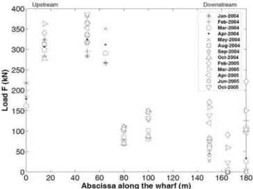
In order to give an overview of the distribution of loading in tie-rods along the wharf, we illustrate (Figure 3) a representation of several measures ob-tained at given dates. The mean values computed from data collected during a month are plotted in view to smooth effects of the lunar period. We can observe a great scatter in space and time that comes on the one hand from embankment loading and con-ditions of building and on the other hand from sea-sonal cycles of the tide (for more details see Yáñez-Godoy, 2004).
Figure 3. Distribution of the mean monthly loads measured in the tie-rods along the wharf
4.2 Correlation and hypothesis on the
behavior
Tie-rods present sensitivity to tide level (Verdure, 2004 and Yáñez-Godoy, 2004) and it is directly lin-ked to the stiffness of the set “soil-rod-anchoring plate”. Indeed, for each tide there is a modification of the soil around the tie-rod. From data we deduce the variation of measured loads in the rods,
, corresponding to the water level varia-tions of the Loire,
1 2 F F F = − Δ 1 2 H H H = −
Δ , between two in-stants given and . The interval of selected time corresponds to the periodicity of the measurements (30 minutes). In France, we associate to the oscilla-tion amplitude of semi-diurnal tide a coefficient named tide coefficient CM AR.
1
t t2
Previous studies have shown that the ratio has a great scatter for a given tie-rod for low conditions ( ) (Yáñez-Godoy, 2004). In fact this scatter is as large when analysing the variation of the loading in a given tie-rod with time than when studying the loading in several tie-rods at a given time. For these conditions, it cannot be considered as representative of the tie-rod. For high tide levels, the quasi-linear correlation between the load in the rods and the variation of the water level is shown to characterize tie-rods behavior. This relationship is shown in Figure 4 that plots this load-ing durload-ing a fallload-ing tide for 7 tie-rods ( ). This paper aims to characterize the behavior of tie-rods for high CM AR: 6 values are se-lected from 95 to 100. Coefficients higher than 100 occur rarely and few data are available.
H F Δ Δ / CM AR CM AR<80 100 = CM AR CM AR
Interest of studying high coefficient tide is for performing studies of structural reliability in case of extreme storm loading (Yáñez-Godoy et al., 2006).
Figure 4. Variation of the measured normal load in the tie-rods in relation to water level variation of the river Loire for a falling tide (CMAR = 100)
F
Δ
H
Δ
5 STOCHASTIC AND MECHANICAL MODELLING
5.1 Stochastic modeling
Let us consider the stochastic process of loading variation during a tide of coefficient CM AR:
CM AR
F
Δ where CM AR∈
{
95; 96; 97; 98; 99; 100}
. This is a stochastic process discrete in space and in time:(
x t CM AR)
F i, j,θjΔ where is the position of the rod, the time when CM AR occurs and
i
x
j
t θj the
event. The correlation of with time is very fair and we assume a white-noise type process at the time level. Then:
CM AR F Δ
(
x t CM AR)
F(
x CM AR)
F i, j,θj =Δ i,θj Δ (1)It leads to assume that at each time , a new event
j
t
j
θ of the same variable is obtained. Let us consider the structure of this stochastic process with space. We assume here that a single set of me-chanical random variables governs this stochastic process.
( )
xiF Δ
In view to identify this set of random variables and to be consistent with this assumption, a post-processing of the samples is performed. In fact the scatter of the mean value of ΔF
(
xi,θj CM AR)
issig-nificant (Figure 5). This bias is explained through the fair size of samples and the error of measurement which is around 10 [kN].
Figure 5. Variation of the measured loads in the tie-rods along the wharf, during falling tides with CMAR = 100
Let us consider μΔFCM AR, the spatial average of the expected value of ΔF
(
xi,θj CM AR)
, defined by(
(
∑
= Δ = Δ n i j i CM AR F E F x CM AR n 1 , 1 θ μ))
, (2)where n is the number of tie-rods. By denoting
(
x CM ARF* i,θj
Δ
)
the centered random variable as-sociated to ΔF(
xi,θj CM AR)
, each variable(
x CM AR)
F i,θj Δ can be written:(
CM AR)
E(
F(
x CM AR)
)
F(
CM AR)
(3) F x ,θj i,θj xi,θj * i = Δ +Δ ΔWe consider the following approximate expan-sion for ΔF
(
xi,θjCM AR)
:(
CM AR)
F(
CM ARF xi,θj ≅μ FCM AR +Δ * xi,θj
Δ Δ
)
(4)This expansion allows filtering the fluctuations on the mean value: this bias is in fact mainly due to the low size of samples.
5.2 Mechanical modeling
A high linear correlation between the load in the rods and the variation of the water level is noticed as showed in Figure 4. This linearity is used to define a tangent modulus that represents overall stiffness of the set “soil-rod-anchoring plate” for high tide lev-els. The aim of mechanical modeling is to provide robust transfer functions that allows to identify k
( )
θfrom the random variables defined in (6) for each coefficient . We have developed two me-chanical models in order to represent spatial behav-ior along the wharf subjected to horizontal loading: the first one is based on a 3D finite-element model and the second one, a 2D model, which parameters are identified from the first one but is based on the beam theory. In aim of reducing computational costs, the second one is used in the following.
CM AR
6 IDENTIFICATION OF TIE-RODS STIFFNESS 6.1 Steps of the flow-chart
In view to identify the variable k
( )
θ representing the tie-rods stiffness, the three following steps are considered after the transformation (4):(i) estimation of a deterministic embankment loa-ding, called tide loading in the following, during a tide of given coefficient CM AR, by know-ing the loads in tie-rods and deterministic stiffness
, CM AR TL F , Δ d k
(ii) computation of each event of k
(
θCM AR)
by knowing the tide loading and the modified distribu-tion of ΔFCM AR according to equation (4),(iii) identification of this distribution by using stochastic chaos.
Note that step (i) is needed because of the lack of knowledge on the earth pressure loading (Verdure et al. 2003, Verdure 2004, Verdure et al. 2005). The deterministic value of is taken at value 61.9 [MN/m]: it is a mean “reasonable” value because it corresponds to the stiffness of a tie rod perfectly embedded in the anchoring plate without soil. In fact presence of the soil tends to increase the stiffness when the possible elastic-displacement of the an-choring plate decreases this stiffness.
d
k
6.2 First Step: estimation of the tide loading Following the flow-chart detailed in sub-section 6.1, the tide loading ΔFTL,CM AR is computed by
in-verse analysis. The corresponding optimization pro-blem is presented in (5).
(
)
(
)
⎟⎟ ⎠ ⎞ ⎜ ⎜ ⎝ ⎛ Δ Δ − = Δ∑
= Δ n i CM AR TL i c CM AR F CM AR TL F x F F CM AR TL 1 2 , 10 max , , ar gmin ; , μ (5) where Fc(
xi FTL CM AR)
, ; ΔΔ is the variation of loading in the tie-rod of abscissa xi resulting from a
compu-tation with the deterministic model (see section 5.2) with a tide loading ΔFTL,CM AR and a deterministic
stiffness of tie-rods of 61.9 [MN/m]. Note that the mean variation of loading μCM AR,max10 is computed
from the 10 maximum values of available events: it allows to compute to use the same sample size what-ever the coefficient CM AR. This problem is solved using a method of order 0 called simplex (Nelder et al. 1965).
6.3 Second step: building of the sample for k For a given coefficient CM AR and by knowing
CM AR TL
F ,
Δ computed from (5) and the post-processed sample of ΔF
(
xi,θj CM AR)
deduced from(4), each event k
(
θj CM AR)
is solution of theoptimi-zation problem (6).
(
)
(
(
)
( ))
2 1 i, ; x min ar g ⎟⎟ ⎠ ⎞ ⎜ ⎜ ⎝ ⎛ Δ − Δ =∑
= n i i c j k jCM AR F CM AR F x k kθ θ (6) where F(
xi k)
c ;Δ is the variation of loading in tie-rod of abscissa resulting from a computation with the deterministic model and with stiffness .
i
x
k
The set of events for k
(
θCM AR)
is thus deduced from the solution of m inversed problem where m is the size of samples ΔFCM AR(
xi,θjCM AR)
. This prob-lem is solved using the same simplex algorithm as above.By assuming that each coefficient CM AR in the range [95; 100] has the same probability of occur-rence, the distribution of variable k
( )
θ is composed of by all events k(
θj CM AR)
, whatever CM AR. Thisdistribution is given on figure 6. The two first statis-tical moments μk and σk are respectively 32.24 [MN/m] and 13.07 [MN/m].
Figure 6. Distribution of k
7 MODELLING USING POLYNOMIAL CHAOS 7.1 Formulation of the problem
When distribution of variables don’t follow a pre-defined probability density function and in view to systematize the identification from a data base and the stochastic computations, methods are now avail-able (Desceliers et al. 2006, Ghanem et al. 2006, Sa-kamoto et al. 2002). We use here the estimate of maximum likelihood for the identification of poly-nomial chaos decomposition (Desceliers et al. 2006). Then the problem is to find the coefficients ki of the
one-dimension polynomial chaos decomposition (7).
( )
θ( )
ξ( )
θ∑
(
ξ(
θ = = = p i i ih k k k 0))
(7)where p is the order of the polynomial chaos de-composition, ξ
( )
θ the Gaussian germ, i.e. a stan-dardized normal variable and the Hermite poly-nomial of degree .i
h i
By using the maximum likelihood method, coef-ficients are solution of the optimization problem (8). i k
( )
κ( )
κ κ L L =ar gmin (8)where κ is the vector of components (
i
k
[
k ,...,0 kp]
=
κ ) with dimension
(
, and is the likelihood function (9).)
)
1 + p L( )
∏
(
( )
= = N j j k k p L 1 ; κ θ κ (9)where N is the size of the sample of k
( )
θj (see 6.3) and pk( )
.; κ is the probability density function of the variable k( )
θ defined in (7), depending on the set of polynomial chaos coefficients.7.2 Algorithm for solution
First the likelihood function (9) takes very fair values very close to the numerical precision. Then the problem (8) is modified in (10).
( )
(
κ)
(
( ( ))
κ)
κ L ogL L L og = − − ar gmin (10)In view to systematize the algorithm it is sug-gested (Desceliers et al. 2006) to work in a standard-ized space by using properties of polynomial chaos and of the decomposition by using (11) (Ghanem et al. 1991). nor m L2
( )
( )
(
)
⎪ ⎩ ⎪ ⎨ ⎧ = = =∑
= p i k i k k k k 1 2 2 0 Var ξθ σ μ (11)where μk and σk are respectively the statistical
av-erage and standard deviation of variable k
( )
θ . They are computed from the experimental sample of k( )
θobtained in 6.3. The first condition reduces the num-ber of unknown coefficients to p and the second one allows to search other coefficients on an hyper-sphere with radius σk. More over, by denoting
the quantity * i k k i
k /σ the conditions (11) become
( )
⎪ ⎩ ⎪ ⎨ ⎧ = =∑
= p i i k k k 1 2 * 0 1 μ (12)These new conditions allow to search p coeffi-cients
[
k1*; ...; ki*; ...; kp*]
on a hyper-sphere withradius 1. This last condition is interesting for the op-timization of algorithms. Note that for p =1 the so-lution is the standardized normal probability density function.
A basic random search algorithm is used for solv-ing (10) by knowsolv-ing (12). It is based on Monte Carlo simulations.
7.3 Solution of the identification
Let us first consider a polynomial chaos of order 2. The solutions ki* and ki are given in table 1.
Table 1. Coefficients for a polynomial chaos of order 2
* i k [MN/m] ki [MN/m] 0 k 32.24 * 1 k 0.9891 k1 12.93 * 2 k 0.1475 k2 1.93
The mean and standard deviation of k
(
ξ( )
θ)
are identical to those computed in 6.3 from the statistical distribution.Figure (7) illustrates the variations of −L og
(
L( )
κ)
on the circle with radius 1. Note that coefficients can be either positive or negative due to the second con-dition of (12) and the fact that ξ
( )
θ is a standardized normal variable.Figure 7. Variations of −L og(L( )κ ) with the couple
(
*)
2 * 1; kk .
By using the second property in (12), we can in-troduce an angular parameter ϕ (13).
[
π ϕ ϕ ϕ 2 ; 0 ) sin( ) cos( * 2 * 1 ∈ ⎪⎩ ⎪ ⎨ ⎧ = = wi th k k]
)
(13) The evolution of −L og(
L( )
ϕ is presented onfig-ure 8 where we can localize the minimum of the likelihood function.
Figure 8. Variations of −L og(L( )ϕ ).
The pdf of the obtained polynomial chaos decom-position is plotted on figure 9 and shows a conven-ient fitting of the statistical distribution of k.
Figure 9. Statistical distribution of k and fitting with a poly-nomial chaos of order 2.
Let us now consider a polynomial chaos of order 3. The solutions ki* and ki are given in table 2.
Table 2. Coefficients for a polynomial chaos of order 3
* i k [MN/m] ki [MN/m] 0 k 32.24 * 1 k 0.9923 k1 12.97 * 2 k 0.1163 k2 1.52 * 3 k 0.0426 k3 0.56
The mean and standard deviation of k
(
ξ( )
θ)
are identical to those computed in 6.3 from the statistical distribution. Coefficients and are very close to those obtained from order 2 and coefficient is negligible. It leads to conclude that the polynomial chaos of order 2 is sufficient. A convergence test can be developed with the convergence of these coeffi-cients or of the variance of the solution.1
k k2
3
k
8 CONCLUSIONS
This paper first presents the complexity of wharf building and behavior. The strategy of monitoring which aims to characterize this behavior is then ad-dressed. A mechanical modelling is addressed to un-derline the main variables that govern the scatter in loading on tie-rods.
It allows to identify the best distribution for these basic variables. An original identification is sug-gested: it is based both on maximum likelihood es-timates and decomposition on polynomial chaos. This method avoids to assume a prior distribution type. A second order and third order polynomial chaos are considered for the illustration.
REFERENCES
Del Grosso A., Inaudi D. and Lanata F., (2000), “Strain and displacement monitoring of a quay wall in the Port of Genoa by means of fibre optic sensors”, 2nd ENPC Euro-pean Conference, Champs-sur-Marne, France, 3-6 July, on CD-Rom.
Desceliers C., Soize C., Ghanem R. (2006), “Identification of chaos representations of elastic properties of random media using ex-perimental vibration tests”, Computational Mechanics, Springer Berlin / Heidelberg, Mars, pp. 831-838.
Ghanem R. and Spanos P., (1991), “Stochastic finite elements: a spectral approach”, Courier Dover Publications, 224 p.
Ghanem R.G., Doostan A. (2006), “On the construction and analysis of stochastic models: characterization and propagation of the er-rors associated with limited data”, Journal of Computational Phys-ics, Volume 217, issue 1, Septembre, Academic Press Profes-sional, Inc., pp. 63-81.
Gattermann J., Bergs T. and Rodatz W., (2001), “Modified in-strumentation and results of stress and deformation moni-toring at the new quay wall construction – Container Ter-minal Altenwerder, Port of Hamburg”, 8th International Conference on Structural Safety and Reliability, California, USA, 17-21 June, on CD-Rom.
Magnan J-P., (2006), “Eurocode 7: calcul géotechnique”, Techniques de l'ingénieur, Construction, Editor ETI - Sci-ences et Techniques, C 240, pp. 1-8.
Marten S., Delattre L., Nguyen and Burgeois E., (2004), “The new deep water quay "Port 2000" of Le Havre, France : field monitoring and performance prediction”, Numerical Models in Geomechanics – NUMOG IX, London, pp. 565-571.
Nelder J. and Mead R., (1965), “A simplex method for function minimization”, The computer journal 7.
Rodatz W., Maybaum G. and Gattermann J., (1995), “Pressure and deformation measurements at two retaining walls at the
port of Hamburg”, 4th International Symposium Field Measurements in Geomechanics (FMGM 95), Bergamo, It-aly, pp. 291-299.
Sakamoto S. and Ghanem R., (2002), “Simulation of Multi-dimensional non-gaussian non-stationary random fields”, Probabilistic Engineering Mechanics, 17, n° 2, April, Elsevier Ed., pp. 167-176.
Verdure L., Casari P. and Schoefs F., (2003), Joint use of in-strumentation and probabilistic modelling applied to a con-tainer wharf, Proc. 9th Inter. Conf. On Applications of Sta-tistics and Probability in civil engineering – ICASP 9, San Francisco, USA, on CD-Rom.
Verdure L., (2004), “Cadre statistique du suivi en service des ouvrages de génie civil : application à un quai sur pieux”, PhD Thesis, Nantes University, France, 232 p.
Verdure L., Schoefs F., Casari P. and Yanez-Godoy H., (2005), “Uncertainty updating of an on-pile wharf after monitoring”, 9th International Conference on Structural Safety and Reliability – ICOSSAR 2005, Rome, Italy, Au-gusti et al., publishers, June, pp. 1347-1354.
Yáñez-Godoy H., (2004), “Identification d'indicateurs de per-formance d'un quai d'accostage en estuaire”, Research rap-port, Nantes University, France, 110 p.
Yáñez-Godoy H., Schoefs F., Nouy A., Casari P., (2006), ”Ex-treme storm loading on in-service wharf structures : interest of monitoring for reliability updating”, special issue “Fiabi-lité des matériaux et des structures et analyse des risques”, Revue Européenne de Génie Civil, Volume 10 n°5/2006 – Hermès / Lavoisier, pp. 565-581.