HAL Id: hal-00587309
https://hal.archives-ouvertes.fr/hal-00587309
Submitted on 25 Jun 2019HAL is a multi-disciplinary open access archive for the deposit and dissemination of sci-entific research documents, whether they are pub-lished or not. The documents may come from teaching and research institutions in France or abroad, or from public or private research centers.
L’archive ouverte pluridisciplinaire HAL, est destinée au dépôt et à la diffusion de documents scientifiques de niveau recherche, publiés ou non, émanant des établissements d’enseignement et de recherche français ou étrangers, des laboratoires publics ou privés.
On the Dynamic Properties of Flexible Parallel
Manipulators in the Presence of Type 2 Singularities
Sébastien Briot, Vigen Arakelian
To cite this version:
Sébastien Briot, Vigen Arakelian. On the Dynamic Properties of Flexible Parallel Manipulators in the Presence of Type 2 Singularities. Journal of Mechanisms and Robotics, American Society of Mechanical Engineers, 2011, 3 (3). �hal-00587309�
On the Dynamic Properties of Flexible Parallel Manipulators in the
Presence of Type 2 Singularities
Sébastien Briota and Vigen Arakelianb
a Institut de Recherches en Communications et Cybernétique de Nantes (IRCCyN), UMR CNRS 6597
1 rue de la Noë, BP 92101, 44321 Nantes Cedex 3, France
Sebastien.Briot@irccyn.ec-nantes.fr
(corresponding author)
b Département de Génie Mécanique et Automatique - L.G.C.G.M. EA3913 Institut National des Sciences Appliquées (I.N.S.A.)
20 avenue des Buttes de Coësmes – CS 14315 F-35043 Rennes, France
vigen.arakelyan@insa-rennes.fr
Abstract
In the present paper, we expand information about the conditions for passing through Type 2 singular configurations of a parallel manipulator. It is shown that any parallel manipulator can cross the singular configurations via an optimal control permitting the favourable force distribution, i.e. the wrench applied on the end-effector by the legs and external efforts must be reciprocal to the twist along the direction of the uncontrollable motion. The previous studies have proposed the optimal control conditions for the manipulators with rigid links and flexible actuated joints. The different polynomial laws have been obtained and validated for each examined case. The present study considers the conditions for passing through Type 2 singular configurations for the parallel manipulators with flexible links. By computing the inverse dynamic model of a general flexible parallel robot, the necessary conditions for passing through Type 2 singular configurations are deduced. The suggested approach is illustrated by a 5R parallel manipulator with flexible elements and joints. It is shown that a 16th order polynomial law is necessary for the optimal force generation. The obtained results are validated by numerical simulations carried out using the software ADAMS.
Index terms – Singularity, dynamics, parallel manipulators, optimal motion generation,
flexible links.
1 Introduction
There are many studies dealing with the singularity analysis of parallel manipulators and an overview of all the works seems almost impossible within the framework of this paper. Let us disclose the kinematic, kinetostatic and dynamic aspects of singularity through some of them. The analysis of singular configurations has been first discussed from a kinematic point of view [1]–[12]. However, it is also known that, when parallel manipulators have Type 2 singularities [1], they lose their stiffness and their quality of motion transmission, and as a result, their payload capability. Therefore, the singularity zones in the workspace of manipulators may be analyzed not only in terms of kinematic criterions, from the theoretically
perfect model of manipulators without friction and force transmission action, but also in terms of kinetostatic performance [13]–[20]. In this vein, the paper [20] proposes the analysis and design of a Stewart Platform based force–torque sensor in a near-singular configuration. It was shown in this study that various singular configurations can be obtained to get high sensitivity to various combinations of the six components of force and torque.
The further study of singularity in parallel manipulators has revealed an interesting problem that concerns the path planning of parallel manipulators under the presence of singular positions, i.e. the motion feasibility in the neighbourhood of singularities. In this case the dynamic conditions can be considered in the path planning process. One of the most evident solutions for the stable motion generation in the neighbourhood of singularities is to use redundant sensors and actuators [21]–[25]. However, it is an expensive solution to the problem because of the additional actuators and the complicated control of the manipulator caused by actuation redundancy. Another approach concerns with motion planning to pass through singularity [26]–[31], i.e. a parallel manipulator may track a path through singular poses if its velocity and acceleration are properly constrained. This is a promising way for the solution of this problem. However, the studies devoted to this problem have addressed the path planning for obtaining a good tracking performance, but not the physical interpretation of dynamic aspects.
The condition of optimal force generation in rigid parallel manipulators for passing through the singular positions has been studied in [32]. It was shown that any parallel manipulator can pass through the singular positions without perturbation of motion if the wrench applied on the end-effector by the legs and external efforts of the manipulator are reciprocal to the twist along the direction of the uncontrollable motion. The obtained results were validated through experimental tests carried out on the prototype of four-DOF parallel manipulator PAMINSA [33].
This approach has been generalised in the case of rigid-link flexible-joints parallel manipulators [34]. It was shown that the degree of the polynomial law should be different, when the flexibility of actuated joints is introduced into condition of the optimal force generation in the presence of singularity. The numerical simulations carried out using the software ADAMS validated the obtained theoretical results.
The study presented in this paper is the continuation of our previous works [32], [34]. The purpose of this paper is to study the dynamic properties of parallel manipulators having not only flexible joints, but also flexible links.
The paper is organized as follows. The next section presents theoretical aspects of the examined problem, which is analysed using the Lagrangian formulation. The condition of force distribution is defined, that allows the passing of any flexible parallel manipulator through the Type 2 singular positions. In section 3, the suggested solution is illustrated via a 5R planar parallel manipulator having flexible links and joints. Conclusions are presented at the end of the paper.
2 Optimal dynamic conditions for passing through Type 2 singularity
Let us consider a non-redundant parallel manipulator of m links, n degrees of freedom and driven by n actuators. The general Lagrangian dynamic formulation for a non-rigid manipulator can be expressed as [35]:
a a L L q q τ dt d , (1a)
e e L L q q 0 dt d , (1b) where,
- L is the Lagrangian of the manipulator; L = T−V, where T is the kinetic energy and V the
potential energy due to gravitational forces, friction and elasticity;
- a T n a a a [q1,q2,...,q ] q and a T n a a a [q1,q2,...,q ]
q represent the vectors of position and velocity of the actuators, respectively;
- e T n e e e [q1,q2,...,q ] q and e T n e e e [q1,q2,...,q ]
q represent the vectors of position and velocity of the elastic coordinates (deformations of links and joints);
- is the vector of the actuators efforts.
In general, for parallel manipulators, the potential and kinetic energies do not explicitly depend both of the actuated variables qa and elastic coordinates qe, but also from the positions
x and velocities v of the payload. Therefore it is preferable to rewrite Eq. (1) using the
Lagrange multipliers [35], as follows:
λ B W τ b T , a a L L q q Wb dt d (2a) λ C W 0 c T , e e L L q q Wc dt d (2b) where is the Lagrange multipliers vector, which is related to the wrench Wp applied on the
platform by: p W AT , x v Wp L L dt d (3) and, - T z y x, , , , , ] [ x and T z y x, , , , , ] [
v are vectors containing the end-effector trajectory parameters and their derivatives, respectively; x, y, z represent the position of the controlled point in the global frame and and the rotation of the platform about three axes a, a and a. Vector x depends on both rigid coordinates qa and elastic coordinates qe.
- A, B and C are three matrices relating the vectors v, q and e q according to a
e
a Cq
q B
Av . They can be found by differentiating the closure equations fi(x, qa, qe) = 0 (taking into account the rigid as well as the elastic coordinates [35]) with respect to time. In the hypothesis of small elastic displacements (qe 0), matrices A and B may be found
assuming that the robot is composed of rigid links only.
- Wp is the wrench applied on the platform by the legs and external forces expressed along
axes a, a and a [36].
Expressing Wp in the base frame, one can obtain: p R q b J W W τ T 0 a , (4a) p R q c J W W 0 T 0 e , (4b)
where J
R A Bq
1
0
a is the square Jacobian matrix between the twist t of the platform (expressed in the base frame) and the vector q of actuators velocities, a J
A CR q 1 0 e is the non-square Jacobian matrix between twist t of the platform (expressed in the base frame) and the vector q of deformations velocities, e R0AAD is the expression of matrix A in the base
frame, where D is a transformation matrix, of which expression is given in [37].
For any prescribed trajectory x(t), the values of vector qa can be found using the inverse kinematics and dynamics. Thus, taking into account that the manipulator is not in a Type 1 singularity [1], i.e the mechanism is at a configuration where it loses one DOF, the terms Wb,
Wc and R0Wp can be computed [38]. However, for a trajectory passing through a Type 2
singularity, the determinant of matrix AR0 vanishes. Numerically, the values of the efforts
applied by the actuators become infinite. In practice, the manipulator either is locked in such a position of the end-effector or it can not follow the prescribed trajectory.
As it is mentioned above, in a Type 2 singularity, the determinant of matrix AR0
vanishes. In other words, at least two of its columns are linearly dependant [37]. So, one may obtain such a relationship:
0 0
R T R T T
s s
A t 0 t A 0 , (5)
where the vector ts represents the direction of the uncontrollable motion of the platform in a
Type 2 singularity.
Then, by dot-multiplying both sides of (3) by ts and taking into account (5), we obtain
0 0
R
T T
s
t A λ , (6)
which also implies that
0 0
R
T
s p
t W , (7)
Thus, (7) corresponds to the scalar product of vectors ts and p R0W .
Thus, in the presence of a Type 2 singularity, it is possible to satisfy conditions (7) if the
wrench applied on the platform by the legs and external efforts R0Wp are reciprocal to the direction of the uncontrollable motion ts. Otherwise, the dynamic model is not
consistent. Obviously, in the presence of a Type 2 singularity, the displacement of the end-effector of the manipulator has to be planned to satisfy (7). Therefore, our task will be to achieve a trajectory which will allow the manipulator passing trough the Type 2 singularities, i.e. which will allow the manipulator respecting condition (7).
In the next section, an example illustrates the obtained results discussed above. This example presents a planar 5R flexible parallel manipulator.
3 Illustrative example
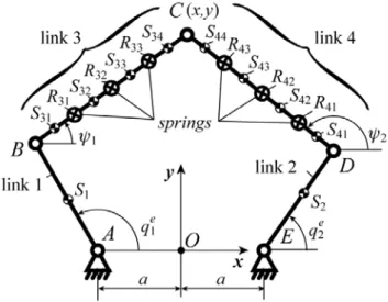
In the planar 5R parallel manipulator, as shown in Fig. 1, the output point is connected to the base by two legs, each of which consists of three revolute joints and two links. In each of the two legs, the revolute joint connected to the base is actuated. Thus, such a manipulator is able to position its output point in a plane.
As shown in Fig. 1, the input joints are denoted as A and E. The orientation of elements 1 and 2 are denoted e
q1 and q2e, respectively. The common joint of the two legs is denoted as C,
which is also the output axis with controlled parameters x = [x, y]T. A fixed global reference system xOy is located at the middle of segment AE with the y-axis normal to AE and the x-axis directed along AE. The lengths of the links AB & DE and BC & CD, are respectively denoted as Lp and Ld.
Actuators 1 and 2 are connected to links 1 and 2, respectively, via Harmonic Drive® systems which are represented by a model similar to that given in [39]. The position of actuator i is denoted as a
i
q . It is assumed that the actuator i is capable to deliver a couple i to
the motor shaft, which is elastically coupled to the link i of the robot (i = 1 or 2). The flexibility of the drive system is modeled by a torsion spring with stiffness k1. The gear ratio is denoted n. Ia is the axial moment of inertia of the motor i plus the Harmonic drive system.
Figure 1. Kinematic chain of the planar 5R parallel manipulator.
(a)1 = 2 (b)1 = 2
Figure 2. Type 2 singular configurations of the planar 5R parallel manipulator.
The deformations of the robot links 3 and 4 are modeled by adding virtual torsion springs at points Rij (i = 3, 4 and j = 1 to 3), such as elements 3 and 4 are decomposed into four sub-elements, denoted as elements iv (i = 3, 4 and v = 1 to 4), with identical lengths and inertia
properties. The stiffness of these springs is denoted as k2. The displacement of the spring mounted at point Rij will be denoted as ij.
The singularity analysis of this manipulator shows that the Type 2 singularities appear when links 3 and 4 are parallel [40] (Fig. 2). In both cases, the gained degree of freedom is an infinitesimal translation perpendicular to the links 3 and 4.
Taking into account that the gravity is directed along z axis (perpendicular to the plane of motions), the expression of the potential energy V may be written as:
1 2
0.5 ( / ) (T / ) T a e a e V k q nq q nq k ε ε . (8) where qa = [ a q1 ,q2a]T, qe = [ e q1,q2e]T and = [31,2,3, 41,2,3]T. The expression of the kinetic energy is2 4 4 1 3 1 0.5( ( ( ) ( ) ( ) ( ) ( ) ( )) ) T T T T T a a a p e e d T T T p Si Si d Sij Sij i i j T I I I m m
1 1 1 2 1 2 1 2 3 1 2 3 q q q q ψ ψ ψ ε ψ ε ψ ε ε ψ ε ε ψ ε ε ε ψ ε ε ε v v v v (9) where - [ , ]T 2 1 ψ is the vector of the angular velocities of elements 3 and 4,
- [ 3 , 4 ]T j j j
ε , j = 1 to 3
- vSi is the translational velocity vector of the centre of masses of element i (i = 1, 2); the centre of masses is located at the middle of the considered segment.
- vSij is the translational velocity vector of the centre of masses of element ij (i = 3, 4 and j = 1 to 3); the centre of masses is located at the middle of the considered segment.
- mp is the mass of the proximal links (elements 1 and 2), md is the mass of each sub-elements of the distal links (elements ij, (i = 3, 4 and j = 1 to 4));
- Ip is the axial moment of inertia of the proximal links (elements 1 and 2), Id is the axial moment of inertia of each sub-elements of the distal links;
The expressions of vectors vSi are:
sin 0.5 cos e e i Si p i e i q L q q v , for i = 1, 2 (10a) sin sin cos 8 cos e i e i d Sij p i e i i i q L L q q v , for i = 1, 2 and j = 1 (10b) ( 1) ( 1) ( 1) ( 1) sin( ) sin ( ) cos( ) cos 8 8 i i j i d d Sij Si j i i i j i i j i L L v v , for i = 1, 2 and j = 2 (10c) ( 2) ( 1) ( 2) ( 2) ( 2) ( 1) ( 2) ( 1) ( 2) ( 1) sin( ) ( ) cos( ) 8 sin( ) ( ) cos( ) 8 i i j d Sij Si j i i j i i j i i j i j d i i j i j i i j i j L L v v , for i = 1, 2 and j = 3 (10d)
( 3) ( 2) ( 1) ( 3) ( 2) ( 3) ( 2) ( 3) ( 2) ( 1) ( 3) ( 2) ( 1) ( 3) ( 2) ( 1) sin( ) ( ) cos( ) 8 sin( ) ( ) cos( ) 8 i i j i j d Sij Si j i i j i j i i j i j i i j i j i j d i i j i j i j i i j i j i j L L v v , for i = 1, 2 and j = 4 (10e)
Introducing (10a, b, c, d, e) into (9), the dynamic model can be obtained from (2) and (3): 2 T k ε ε p W J W ε 0, (11)
1 / e e T a e k n q q p W J W q q 0, (12) and Iaqak1(qeqa/n)/n. (13)The terms that appear in this model are described in the appendix.
For given trajectory x(t), the deformations (t) may de deduced from (11). However, this equations is difficult to solve analytically, therefore an iterative resolution of the system is used [38]. Once (t) is known, the displacements, velocities, accelerations and other time derivatives of the passive and active variables qe and may be found using the dynamic model equations and the loop closure equations, which are given in the appendix. Then, from (12), the values of qa are found:
1 ( ) / e e T a n q q p k n e q W J W q . (14)
Finally, the input torques can be computed using (13).
From (11), it appears that the deformations depends on the position x, velocity x and acceleration x of the end-effector. As a result, ε depends on the end-effector position x, velocity x, acceleration x , jerk x and its first derivative x(4). Thus, qa also depends on the same parameters. As a result, from (13), it can be shown that the input torques depends on the end-effector position, velocity, acceleration, jerk and its first, second and third derivatives with respect to time. Therefore, a thirteen-degree polynomial has to be applied as a control law when the end-effector is not in singular configuration.
In order to avoid infinite values of the input torques when crossing a Type 2 singularity, Eq. (7) has to be satisfied. From matrix A (see appendix), one can find that the twist of the infinitesimal displacement in the singularity can be written under the form:
T ] cos , sin [ 1 1 s t (15)
Thus, the examined manipulator can pass through the given singular positions if the wrench Wpdetermined by (14) is reciprocal to the direction of the uncontrollable motion ts
described by (15). However, the difficulty remains into the fact that, introducing Wp (see
appendix) into (7) leads to a condition, which depends not only on the end-effector position, velocity and acceleration, but also of variables , ε and ε, which at any computation step can only be iteratively found. Therefore, contrary to our previous papers [32][34] in which the polynomial laws able to achieve condition (7) were defined analytically, in this case, this law
can only be found by using numerical simulation algorithms. An example of the use of such algorithm is given below.
Let us now determine the trajectory, which makes it possible to satisfy condition (7) for the manipulator with following parameters of links: a = 0.2 m, Lp = Ld = 0.25 m, mp = 1.75 kg, md = 1.8 kg, Ip = 1.18.10-2 kg.m², Id = 1.5.10-4 kg.m², Ia = 0.064.10-4 kg.m², k1 = k2 = 800 Nm/rad, n = 50.
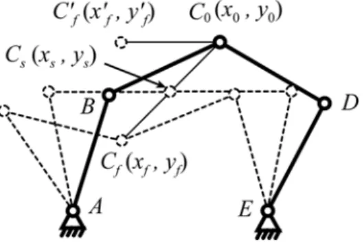
With regard to the prescribed trajectory generation, the point C should reproduce a motion along a straight line between the initial position C0 (x0, y0) = C0 (0.1, 0.345) and the final point
Cf (xf, yf) = Cf (–0.1, 0.145) in tf = 1 s (Fig. 3). However, the manipulator will pass by a Type 2 singular position at point Cs (xs, ys) = Cs (0, 0.245) (Fig. 3).
Figure 3. Initial, singular and final positions of the planar 5R parallel manipulator. The trajectory can be expressed as follows:
) ( ) ( ) ( ) ( ) ( ) ( 0 0 0 0 y y t s y x x t s x t y t x f f x (16)
where s(t) is a polynomial, that should respect the following conditions:
s (t0) = 0, (17) s (tf) = 1, (18) 0 ) ( ) (t0 s tf s , (19) 0 ) ( ) (t0 s tf s , (20) 0 ) ( ) (t0 s tf s , (21) 0 / )) ( ( / )) ( (s t0 dt d s t dt d f , (22) 0 / )) ( ( / )) ( ( 2 2 2 0 2 dt t s d dt t s d f , (23) 0 / )) ( ( / )) ( ( 3 3 3 0 3 dt t s d dt t s d f , (24)
s (ts = 0.5 s) = 0.5, (25) 0 ) (ts s , (26) and tTWp 0 s . (27)
There are seventeen conditions, therefore s(t) should be at least a sixteen-degree polynomial.
Boundary conditions (17) to (26) are directly linked to the expression of the polynomial, whereas (27) involve the computation of the entire dynamic model, therefore, one way to find the polynomial is to express conditions (17-27) as the following optimization problem:
a p W t a) min ( T s f (28)
subject to constraints (17-26), where a is a vector regrouping the coefficients of the polynomial s(t). It is obvious that such formulation does not imply a 100% guaranty that the function f(a) will be null at the end of the optimization step. However, in general, the simulations have shown that, even if the minimization problem (28) may not yield a zero result, it was possible to obtain a value close to zero.
A way to solve this problem is to use the goal attainment programming (function “fgoalattain” in Matlab). The goal attainment optimization allows generating specific Pareto-optimal solutions. Let us apply the goal-attainment technique that yields the following nonlinear programming formulation:
a , min (29) subject to i h h f w f(a) i i0; i(a) i0; (30) where ( ) 0 i i h
h a represents the constraints (17-26). Here, is an unrestricted scalar variable,
0
i
w are designer selected weighting coefficients, and f are the goal to be realized for i0
each design objective. In this formulation, minimization of tends to force the specifications to meet their goal. If, at the solution point, is negative, the goals have been over-attained; if
is positive, then the goals have been under-attained. The method is appealing since it is possible for the user to specify unrealizable objectives and still obtain a solution which represents a compromise. More detailed information about the goal-attainment optimization can be found in [41].
Using the “fgoalattain” function in Matlab, with specified constraints (17-26) and objective (28), the following polynomial has been found:
7 8 9 10 11 12 13 14 15 16 7099.0 52152.8 160698.1 252912.5 173271.6 60944.0 217870.6 179095.5 68776.9 10605.7 s t t t t t t t t t t t (31)This polynomial will be implemented into the dynamic model of the manipulator in order to verify that it allows the passing through the Type 2 singularity. The simulations have been carried out using the software ADAMS.
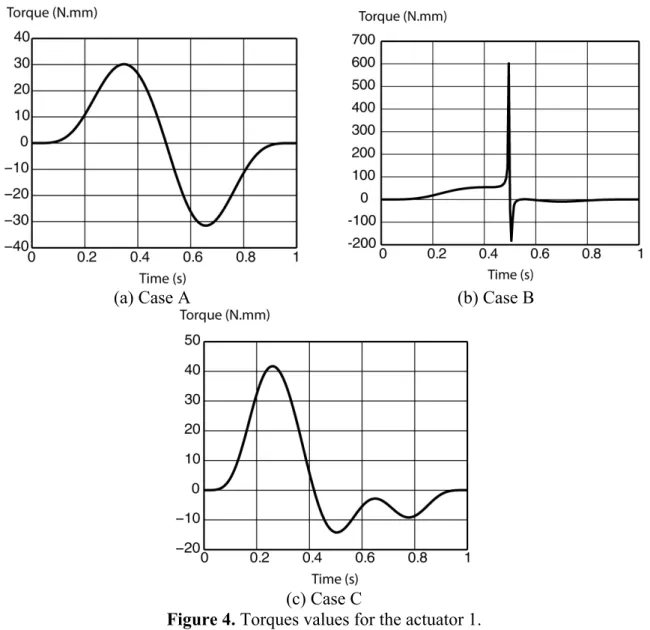
In order to compare the different cases of trajectory planning, in Figs. 4 and 5 are given the values of the input torques obtained using the software ADAMS for the following numerical simulations:
A: a trajectory between points C0 and C’f (x’f, y’f) = C’f (–0.1, 345) (Fig. 3) without meeting any singularity. For such a case, a thirteenth order polynomial law has been defined from conditions (17-24). The obtained
1716 7 9009 8 20020 9 24024 10 1638011s t t t t t t
12 13
6006t 924t
polynomial law is used for the trajectory planning out of the singular zone of the manipulator. In this case the values of the input torques are finite.
B: the same thirteenth order polynomial law
1716 7 9009 8 20020 9 24024 10s t t t t t
11 12 13
16380t 6006t 924t
is usedfor the trajectory planning between C0 and Cf inside the singular zone of the manipulator. In this case the values of the input torques close to the singular positions tend to infinity.
C: the sixteenth order polynomial law of Eq. (31) for the trajectory planning of the manipulator inside the singular zone. The obtained results show that the values of the input torques are finite.
(a) Case A (b) Case B
(c) Case C
It is interesting to observe the manipulator’s behaviour for the simulated cases. The first law, which is a thirteenth order polynomial, assumes the prescribed motion without perturbation of torques outside of the singular zone. The same law does not provide the stable motion in the presence of singularity. The sixteenth order polynomial law re-establishes the stable motion for passing trough the singular position.
(a) Case A (b) Case B
(c) Case C
Figure 5. Torques values for the actuator 2.
4 Conclusion
In our previous work, we have shown that any parallel manipulator can pass through the singular positions without perturbation of motion if the wrench applied on the end-effector by the legs and external efforts is reciprocal to the twist along the direction of the uncontrollable motion [32]. This condition was applied to the rigid-link manipulators. The obtained results showed that the planning of motion for assuming the optimal force generation can be carried out by an eight order polynomial law. In [34] the rigid-link flexible-joint manipulators have been studied. It was shown that the degree of the polynomial law should be different, when the flexibility of actuated joints is introduced. The obtained results disclosed that the planning
of motion for assuming the optimal force generation in the rigid-link flexible-joint manipulators must be carried out by a twelfth order polynomial law.
In this paper, we have expanded the information about the dynamic properties of parallel manipulators in the presence of Type 2 singularity by including in the studied problem the link flexibility. The obtained results have shown that the planning of motion for assuming the optimal force generation in the manipulators with flexible links must be now carried out by a sixteenth order polynomial law.
The suggested technique was illustrated by a 5R planar parallel manipulator. The obtained results have been validated by numerical simulations carried out using the software ADAMS.
References
[1] C.M. Gosselin, J. Angeles, Singularity Analysis of Closed-Loop Kinematic Chains, IEEE
Transactions on Robotics and Automatics, 6 (3) (1990) 281-290.
[2] D. Zlatanov, R.G. Fenton, B. Benhabib, Singularity Analysis of Mechanisms and Robots via a Velocity-Equation Model of the Instantaneous Kinematics, Proceedings of the 1994
IEEE International Conference on Robotics and Automation, 2010, 980-991.
[3] M. Zein, P. Wenger, D. Chablat, Singular Curves in the Joint Space and Cusp Points of 3-RPR parallel manipulators”, Robotica, 25 (6) (2007) 717-724.
[4] M. Zein, P. Wenger, D. Chablat, Non-Singular Assembly-mode Changing Motions for 3-RPR Parallel Manipulators, Mechanism and Machine Theory, 43 (4) (2008) 480-490. [5] D. Kanaan, P. Wenger, S. Caro, D. Chablat, Singularity Analysis of Lower-Mobility
Parallel Manipulators Using Grassmann-Cayley Algebra, IEEE Transactions on
Robotics, 25 (5) (2009) 995-1004.
[6] D. Zlatanov, I.A. Bonev, C.M. Gosselin, Constraint Singularities of Parallel Mechanisms,” IEEE International Conference on Robotics and Automation (ICRA 2002), Washington, D.C., USA, 2002, May 11-15.
[7] K.H. Hunt, Special Configurations of Robot-Arms via Screw Theory, Robotica, 5, (1987) 17-22.
[8] J.-P. Merlet, Singular Configurations of Parallel Manipulators and Grassmann Geometry,
The International Journal of Robotics Research, 8 (5) (1989) 45-56.
[9] I.A. Bonev, D. Zlatanov, C.M. Gosselin, Singularity Analysis of 3-DOF Planar Parallel Mechanisms via Screw Theory, ASME Journal of Mechanical Design, 125 (3) (2003) 573–581.
[10] M. Husty, C.M. Gosselin, On the Singularity Surface of Planar 3-RPR Parallel Mechanisms, MUSME 2008 Symposium, San Juan, Argentine, 36 (4) (2008) 411-425. [11] S. Bandyopadhyay, A. Ghosal, Analysis of Configuration Space Singularities of
Closed-Loop Mechanisms and Parallel Manipulators, Mechanism and Machine Theory, 39 (5) (2004) 519-544.
[12] S. Briot, I.A. Bonev, D. Chablat, P. Wenger, V. Arakelian, Self Motions of General 3-RPR Planar Parallel Robots, The International Journal of Robotics Research, 27 (7) (2008) 855-866.
[13] Gosselin, C.M., 1992, “The Optimum Design of Robotic Manipulators using Dexterity Indices,” Robotics and Autonomous Systems, Vol. 9(4), pp. 213–226.
[14] N. Rakotomanga, D. Chablat, S. Caro, Kinetostatic Performance of a Planar Parallel Mechanism with Variable Actuation”, 11th International Symposium on Advances in
Robot Kinematics, Kluwer Academic Publishers, Batz-sur-mer, France, 2008, June.
[15] J.-P. Merlet, Jacobian, Manipulability, Condition Number, and Accuracy of Parallel Robots, ASME Journal of Mechanical Design, 128 (1) (2006) 199-206.
[16] J. Angeles, Fundamentals of Robotic Mechanical Systems: Theory, Methods, and Algorithms, 3rd edition, Springer, New York, 2007.
[17] O. Alba-Gomez, P. Wenger, A. Pamanes, Consistent Kinetostatic Indices for Planar 3-DOF Parallel Manipulators, Application to the Optimal Kinematic Inversion, Proc.
ASME 2005 IDETC/CIE Conference, Long Beach, California, September 24-28, 2005.
[18] V. Arakelian, S. Briot, V. Glazunov, Increase of Singularity-Free Zones in the Workspace of Parallel Manipulators using Mechanisms of Variable Structure, Mechanism
and Machine Theory, 43 (9) (2008) 1129-1140.
[19] J. Hubert, J.-P. Merlet, Singularity Analysis through Static Analysis, Advances in Robot
Kinematics, Springer, 2008, 13-20.
[20] R. Ranganath, P. S. Nair, T. S. Mruthyunjaya, A. Ghosal, A Force–Torque Sensor Based on a Stewart Platform in a Near-Singular Configuration, Mechanism and Machine
Theory, 39 (9) (2004) 971-998.
[21] K. Alvan, A. Slousch, On the Control of the Spatial Parallel Manipulators with Several Degrees of Freedom, Mechanism and Machine Theory, Saint-Petersburg, 1 (2003) 63-69. [22] B. Dasgupta, T. Mruthyunjaya, Force Redundancy in Parallel Manipulators: Theoretical
and Practical Issues, Mechanism and Machine Theory, 33 (6) (1998) 724-742.
[23] V. Glazunov, A. Kraynev, R. Bykov, G. Rashoyan, N. Novikova, Parallel Manipulator Control While Intersecting Singular Zones, Proc. 15th Symposium on Theory and
Practice of Robots and Manipulators (RoManSy) CISM-IFToMM, 2004, Montreal.
[24] J. Kotlarski, T. Do Thanh, H. Abdellatif, B. Heimann, Singularity Avoidance of a Kinematically Redundant Parallel Robot by a Constrained Optimization of the Actuation Forces, Proceedings of the Seventeenth CISM-IFToMM Symposium RoManSy, 2008, 435-442.
[25] J. Hesselbach, J. Wrege, A. Raatz, O. Becker, Aspects on the Design of High Precision Parallel Robots, Assembly Automation, 24 (1) (2004) 49-57.
[26] S. Bhattacharya, H. Hatwal, A. Ghosh, Comparison of an Exact and Approximate Method of Singularity Avoidance in Platform Type Parallel Manipulators, Mechanism
and Machine Theory, 33 (7) (1998) 965-974.
[27] B. Dasgupta, T. Mruthyunjaya, Singularity-Free Path Planning for the Steward Platform Manipulator, Mechanism and Machine Theory, 33 (6) (1998) 715-725.
[28] S. Kemal Ider, Inverse Dynamics of Parallel Ma-nipulators in the Presence of Drive Singularities, Mechanism and Machine Theory, 40 (2005) 33-44.
[29] C.K. Kevin Jui, Q. Sun, Path Tracking of Parallel Manipulators in the Presence of Force Singularity, ASME Journal of Dynamic Systems, Measurement and Control, 127 (2005) 550-563.
[30] D.N. Nenchev, S. Bhattacharya, M. Uchiyama, Dynamic Analysis of Parallel Manipulators under the Singularity-Consistent Parameterization, Robotica, 15 (4) (1997) 375-384.
[31] M.H. Perng, L. Hsiao, Inverse Kinematic Solutions for a Fully Parallel Robot with Singularity Robustness, The International Journal of Robotics Research, 18 (6) (1999) 575-583.
[32] S. Briot, V. Arakelian, Optimal Force Generation in Parallel Manipulators for Passing through the Singular Positions, International Journal of Robotics Research, 27 (8) (2008) 967-983.
[33] S. Briot, V. Arakelian, S. Guégan, Design and Prototyping of a Partially Decoupled 4-DOF 3T1R Parallel Manipulator with High-Load Carrying Capacity, ASME Journal of
[34] S. Briot, V. Arakelian, On the Dynamic Properties of Rigid-Link Flexible-Joint Parallel Manipulators in the Presence of Type 2 Singularities, ASME Journal of Mechanisms and
Robotics, (2010), in press.
[35] B.C. Bouzgarrou, P. Ray, G. Gogu, New Approach for Dynamic Modelling of Flexible Manipulators, Proc. IMechE, Part K: Journal of Multi-body Dynamics, 219 (2005) 285-298.
[36] W. Khalil, S. Guegan, A Novel So-lution for the Dynamic Modeling of Gough-Stewart Manipu-lators, Proc. IEEE International Conference on Robotics and Automation, Washington DC., USA, May 11-15, 2002.
[37] J.-P. Merlet, Parallel Robots, Springer, 2nd edition, 2006.
[38] F. Boyer, W. Khalil, Simulation of Flexible Manipulators Using Newton-Euler Inverse Dynamic Model, Proceedings of the 1996 IEEE International Conference on Robotics
and Automation, Minneapolis, Minnesota, April, 1996.
[39] M.W. Spong, K. Khorasani, P.V. Kokotovic, An Integral Manifold Approach to the Feedback Control of Flexible Joint Robots,” IEEE Journal of Robotics and Automation, 1987, 291–300.
[40] X.-J. Liu, J. Wang, G. Pritschow, Kinematics, Singularity and Workspace of Planar 5R Symmetrical Parallel Mechanism, Mechanism and Machine Theory, 41 (2) (2006) 119-144.
[41] P.J. Fleming, A. Pashkevich, Computer Aided Control System Design Using a Multi-Objective Optimisation Approach, Control 1985 Conference, Cambridge, UK, 1985, 174-179.
Appendix
From Eqs. (2, 3), vectors W, Wqe, and Wp can be found:
e e
T T T T T d L L dt p xψ ε εψ q q ψ ψ W J J J J J W v x , (A–1)
2
e p p p e d e e e d L L I m l m dt q q W q F q q , (A–2) d d d L L I m dt ε ε W E F ε ε , (A–3) with
4
d d I m ψ 1 2 3 4 ψ W ψ ε + ε + ε + ε F , (A–4) 11 12 13 21 22 23 [ , , , , , ]T e e e e e e E , (A–5) where, for i = 3, 4 1 3 3 1 2 2 3 i i i i i e , (A–6a) 2 2 2 2 3 i i i i e , (A–6b) 3 3 i i i e , (A–6c)d f f dt ψ F ψ ψ, 4 4 3 1 T Sij Sij i j f
v v (A–7) e e e d f f dt q F q q , (A–8) d f f dt ε F ε ε (A–9)Matrices J and Jqe, of Eqs. (11-13) may be found from the loop closure equations
between x, and qe:
2 2 2 1 1 1 11 11 12 11 12 13 11 12 11 12 13 11 12 13( cos ) ( sin ) (2 cos cos cos
cos 2 cos 2 cos 2 2 ) / 8 0
e e p p d f x a L q y L q L (A–10a)
2 2 2 2 2 2 21 21 22 21 22 23 21 22 21 22 23 21 22 23( cos ) ( sin ) (2 cos cos cos
cos 2 cos 2 cos 2 2 ) / 8 0
e e p p d f x a L q y L q L (A–10b)
from which it comes:
11 12 1 1 21 22 2 2 cos sin 2 cos sin e e p p i e e p p a a x L q a y L q f a a x L q a y L q A x (A–11) 12 1 11 1 22 2 21 2 cos sin 0 0 cos sin e e i p e e e a q a q f L a q a q B q (A–12) 11 12 13 24 25 26 0 0 0 0 0 0 8 i d c c c f L c c c C 0 ε (A–13) with, for i = 1, 2
1 1 1 2 1 2 3 1 2 1 2 3 1 2 3sin sin sin 2sin 2
2sin 2 2sin 2 2 i i i i i i i i i i i i i i i c (A–14a)
2 1 2 1 2 3 1 2 1 2 3 1 2 3sin sin sin 2
sin 2 2sin 2 2 i i i i i i i i i i i i i i c (A–14b)
3 sin 1 2 3 sin 2 1 2 3 sin 2 1 2 2 3
i i i i i i i i i i
c (A–14c)
As a result, it can be found that:
1( )
e e e
q ε
v A Bq Cε J q J ε (A–15)
and also that
1( ) e q B Av Cε , 1( ) e e q B Av Av Cε Cε Bq (A–16)
Matrices T xψ J , T εψ J and e T q ψ
J of Eq. (A–1) may be found from loop closure equations between x, qe, and :
1 cos 1 cos 1 cos( 1 11) cos( 1 11 12) cos( 1 11 12 13) / 4 0
e
p d
g x a L q L
(A–17a)
2 cos 2 cos 2 cos( 2 21) cos( 2 21 22) cos( 2 21 22 23) / 4 0
e
p d
g x a L q L
(A–17b)
3 sin 1 sin 1 sin( 1 11) sin( 1 11 12) sin( 1 11 12 13) / 4 0
e
p d
g y L q L
(A–17c)
4 sin 2 sin 2 sin( 2 21) sin( 2 21 22) sin( 2 21 22 23) / 4 0
e
p d
g y L q L
(A–17d)
from which it comes:
1 0 1 0 0 1 0 1 i g ψ A x (A–18) 1 2 1 2 sin 0 0 sin cos 0 0 cos e e i p e e e q q g L q q ψ B q (A–19) 1 1 1 2 2 2 1 1 1 2 2 2
3sin 2sin sin 0 0 0
0 0 0 3sin 2sin sin
3cos 2cos cos 0 0 0
4
0 0 0 3cos 2cos cos
i d g L ψ C ε (A–20) 1 2 1 2 sin 0 0 sin cos 0 0 cos i d g D L ψ ε (A–21)
As a result, it can be found that:
1 ( ) ( ) e T T e e ψ ψ ψ ψ ψ ψ xψ q ψ εψ ψ D D D A v B q C ε J v J q J ε (A–22) and 1 ( T ) T( ) e e ψ ψ ψ ψ ψ ψ ψ ψ ψ ψ ψ D D D A v B q C ε A v B q C ε D ψ . (A–23)