NUMERICAL MODELING OF UNSTABLE FLOWS IN CONDUCTS WITH VARIABLE GEOMETRY

(1)

Science Arts & Métiers (SAM)

is an open access repository that collects the work of Arts et Métiers Institute of Technology researchers and makes it freely available over the web where possible.

This is an author-deposited version published in: https://sam.ensam.eu

Handle ID: .http://hdl.handle.net/10985/17784

To cite this version :

Sami RAMOUL, Ali FOURAR, Fawaz MASSOUH - NUMERICAL MODELING OF UNSTABLE FLOWS IN CONDUCTS WITH VARIABLE GEOMETRY - Scientific Bulletin - Vol. 80, n°3, p.231-242 - 2018

Any correspondence concerning this service should be sent to the repository Administrator : archiveouverte@ensam.eu

(2)

NUMERICAL MODELING OF UNSTABLE FLOWS IN

CONDUCTS WITH VARIABLE GEOMETRY

Sami RAMOUL1, Ali FOURAR1, Fawaz MASSOUH2

Changes in the system flow of a fluid in a conduct often cause sudden changes in pressure and give rise to so-called unstable flows. So, the study of the phenomenon of unstable flows aims to determine if the pressure in a system is within the prescribed limits, following a perturbation of the flow. In the objective of studying the range of a water hammer, an examination of variations in velocity or flow and pressure resulting from inappropriate operation of the hydraulic system is made. This study presents a numerical modeling of the phenomenon of instable flows in load conducts with variable geometries. The characteristic method is used to solve the governing equations. Thanks to the AFT Impulse industrial program, very interesting and very practical numerical results are obtained to describe the phenomenon of instable flows in conducts with variable geometry. And to more illustrate the graphical presentation two cases are graphically overlay for each of the two types of models (slow closing and rapid closing of the valve).

Keywords: Numerical modeling, unstable flows, water hammer, transient flow, variable section, characteristic method, AFT Impulse software.

1. Introduction

The instable regime in hydraulic installations is a very complex phenomenon. It represents a permanent danger for installations and can occur at any time due to the various manipulations of the elements of this hydraulic system.

The instable regime in the closed conducts is characterized by variations of the pressures, which are often very high or very low. These variations are accompanied by the phenomenon of propagation of the pressure waves that traverse the network for a certain time until their damping and the restoration of the initial regime [1]. This regime is the source of several damages (deterioration of the conducts) which often causes unforeseen equipment and maintenance costs [2].

The objective of this contribution is to treat the most complex case, which means the theory of the hydraulic shock caused by the water hammer in the load

1_{PH.D.Student, Dept of Hydraulics, University of Batna2, Algeria, e-mail:infodoc81@yahoo.com.} 1 _{Prof., Dept.of Hydraulics, University of Batna2, Algeria, e-mail: fourarali05@hotmail.fr}

(3)

conducts with variable geometry, based on the equations of mass conservation and momentum conservation.

To solve these equations, there are many methods which use different simplifying hypotheses and / or resolving procedures, such as analytical, graphic or numerical methods [3]. But given the complexity of the phenomenon, there are not really complete analytical solutions to solve the problem. For instance in the case of Allievi's method [4, 5], which gives us a global solution to the problem, the author does not take into account loss of loads which affects the extent of the phenomenon. Furthermore the approximate graphic methods such as the Schnyder-Bergeron method [6, 7] are not really effective in solving complex cases such as a conduct with several branches, or a conduct with variable characteristics, such as variations of the section, etc. So the numerical methods have taken the relay to allow us to quantify this type of phenomenon.

The objectives of this paper are the study of the propagation causes of the wave in the case of a sudden stop of water supply of the gravity loaded conducts. Put into equation these phenomena by taking as essential points the variations of the sections of conduct and the closing of valves, by use of the numerical method of the characteristics and the AFT Impulse program to solve the equations. To more illustrate the graphical presentation we have graphically overlay two cases for each of the two types of models slow closing and rapid closing of a valve. 2. Basic equations of wave propagation in conducts

The equations which allow us to study one dimension transient that we meet in monophasic flow in conduct are derived by applying the conservations of mass and momentum equations [9]:

Continuity equation 0 2 =   +   x U g C t H (1) Dynamic equation

0

2

1 ₊

₌



+



gD

U

fU

t

U

g

x

H

(2) In which U, H, D, f, g, and C are respectively the average velocity, the piezometric head, conduct diameter, factor of friction, gravity acceleration and velocity of wave pressure.

3. Method of characteristics

Based on the work of [9] and [10], we found that for a partial differential equation (PDE) of the first order, the characteristic method consists in searching for curves (called "characteristic lines" or simply "Characteristics") along which the PDE is reduced to a simple ordinary differential equation (ODE). The

(4)

resolution of the ODE along a characteristic makes it possible to find the solution of the original problem.

By multiplying equation (1) by unknown constant λ, adding it to equation (2), we obtained equation (3): 0 2 2 = +         +   +         +   D U fU t U x U g C t H x H g    (3)

If H=H

( )

x,t and U =U

( )

x,t , then the total derivatives are expressed by

dt dx x H t H dt dH   +   = (4) and dt dx x U t U dt dU   +   = (5) Defining the unknown multiplier λ as

g C g dt dx  2  = = (6) With C g  =  (7) And using Equations (4) and (5), Equation (3) can be written as

0 2 = + + UU D f dt dH C g dt dU W+_{equation (8) for} _C dt dx + = (9) 0 2 = + − UU D f dt dH C g dt dU W- equation (10) For C dt dx₌₋ (11) To understand the meaning of these four equations, figure (1) presents their examination.

Solving the equations (8) and (10) using the characteristic method consists in determining the head H and the velocity U at the point P knowing the initial values at the points R and S. Let UP and HP are the parameters searched at point P.

By multiplying equation (8) by dt and integrating, we obtain:

Fig.1. Characteristic lines [2]. P R S W+ W- x t

(5)

0 2 = + +

_



UUdt D f dH C g dU P R P R P R (12)

(

)

(

)

0 2 = + − + −

_

UUdt D f H H C g U U P R R P R P (13) The term UUdt D f P R



2 can be evaluated as follows:

dt U U dt U U _R _R P R =



(14) For steady conditions the velocity is constant at points R and P

Thus the equation becomes:

0 2 0 0 − + = − + − − D U fU t H H C g t U U _R _R p R p p R p (15) By the same approach, equation (10) can also be written:

0 2 0 0 − + = − − − − D U fU t H H C g t U U _S _S p S p p S P ₍₁₆₎

In these relations, tp - 0 equal to Δt, and when these equations are

multiplied by Δt they become:

C+: 0 2 ) ( ) ( _p − _R + _p− _R + U_RU_R = D t f H H C g U U  (17) And C- : 0 2 ) ( ) ( _p − _S − _p− _S + U_SU_S = D t f H H C g U U  (18)

Each of the characteristic equations can be integrated if:

X =Ct (19) 4. Boundary conditions

The H and U values on the conduct ends are determined using boundary conditions. These conditions are:

(6)

4.1. Condition at the tank boundary

When the conduct outlet from a tank, the value of H remains constant for all times. In this case, it is assumed that:

HP =₁ H₀ (20) This equation is solved simultaneously with the characteristic curve W-. We use Equation (18) to obtain an expression for the velocity

2 2 2 2 1 2 ) ( U U D t f H H C g U U_P = + _o − −  (21) 4.2. Condition at the velocity boundary

If the velocity is known at the downstream end of a conduct, an expression of H is easily found. For example, suppose a valve is closed in a way that caused the velocity to decrease linearly from U0 to zero in T seconds. The Up

equation would be: T t U T t T t U U N N P o P  , 0 0 ), 1 ( 1 1 =   − = + + (22) The equation for HP would be deduced from equation (17)

N N N P N P U U D t f g C N U g C H H N N 1 ( 1 ) ₂  − − − = ₊ + (23)

For any value of UPN+1 including zero.

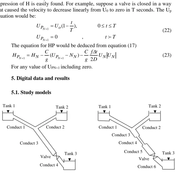
5. Digital data and results 5.1. Study models

Fig. 3. Model 2, conduct of variable diameter. Conduct 6 Tank 1 Tank 2 Conduct 1 Conduct 2 Conduct 3 Conduct 4 Conduct 5 Valve Tank 3

Fig. 2. Model 1, conduct of constant diameter. Tank 1 _{Tank 2}

Conduct 1 Conduct 2

Conduct 3

Valve Tank 3 Conduct 4

(7)

Table 1

Parameters of the conducts and the fluid Steel cond L (m) D (mm) e (mm) k (mm) Ec MPa El MPa tanks H1 (m) H2 (m) H3 (m) Case 1 L1 400 202.71 3.22 0.04572 2*105 ₂₀₅₃ ₁₆₁ ₁₆₁ ₂₀ L2 400 202.71 3.22 L3 1990 202.71 3.22 L4 100 202.71 3.22 L1 400 202.71 3.22 L2 400 202.71 3.22 L3 800 202.71 3.22 Case 2 L4 400 154.05 2.80 L5 790 202.71 3.22 L6 100 202.71 3.22

5.2. Model 1: Conduct of Constant diameter with an analysis of two cases (slow closing and rapid closing of the valve)

0 10 20 30 40 50 60 120 130 140 150 160 170 180 190 200

H

(

m

)

t ( s ) r a p i d c l o s i n g s l o w c l o s i n g

Fig. 4. Variation of head during time in conduct 1 at the mid-point.

Fig. 5. Variation of head during time in conduct 3 at the point of intersection (connection).

0 10 20 30 40 50 60 100 120 140 160 180 200 220 240

H

(

m

)

(8)

Fig. 9. Variation of velocity during time in conduct 3 at the point of intersection (connection). 0 10 20 30 40 50 60 -1.5 -1.0 -0.5 0.0 0.5 1.0 1.5

U

( m

/

s )

0 10 20 30 40 50 60 -50 0 50 100 150 200 250 300 350

H

(

m

)

Fig. 8. Variation of velocity during time in conduct 1 at the mid-point.

0 10 20 30 40 50 60 -0.8 -0.6 -0.4 -0.2 0.0 0.2 0.4 0.6 0.8

U

( m

/

s )

Fig. 7. Variation of head during time in conduct 3 to the valve.

0 10 20 30 40 50 60 -50 0 50 100 150 200 250 300 350

H

(

m

)

(9)

5.2.1. Model 1: comparison between the two cases of the valve closing In the case of rapid closing of the valve more pronounced and faster fluctuations are observed than in the case of slow closing and the fluctuations reach alternately maximum and minimum values. Also the alternation of velocity fluctuations between the positive and negative values explains clearly the movement of the liquid in the two directions of flow caused by water hammer in the conduct. The amplitude of the fluctuations of the velocity in time is very important in the tank then it decreases along the conduct until becoming minimal at the valve. The amplitude of the fluctuations of the piezometric head becomes important along the conduct and reaches maximum values at the valve.

0 10 20 30 40 50 60 -1.5 -1.0 -0.5 0.0 0.5 1.0 1.5

U

( m

/

s

)

Fig. 11. Variation of velocity during time in conduct 3 at the valve.

0 10 20 30 40 50 60 -0.2 0.0 0.2 0.4 0.6 0.8 1.0 1.2 1.4

U

( m

/

s )

(10)

5.3. Model 2: Conduct of variable diameter with an analysis of two cases (slow closing and rapid closing of the valve)

0 10 20 30 40 50 60 120 130 140 150 160 170 180 190 200

H

(

m

)

Fig. 13. Variation of head during time in conduct 3 at the point of intersection (connection).

0 10 20 30 40 50 60 100 120 140 160 180 200 220

H

(

m

)

0 10 20 30 40 50 60 0 50 100 150 200 250 300 350

H

(

m

)

Fig. 15. Variation of head during time in conduct 5 at the valve.

0 10 20 30 40 50 60 0 100 200 300 400

H

(

m

)

(11)

Fig. 16. Variation of velocity during time in conduct 1 at the mid-point. 0 10 20 30 40 50 60 -0.8 -0.6 -0.4 -0.2 0.0 0.2 0.4 0.6 0.8

U

( m

/

s

)

Fig. 17. Variation of velocity during time in conduct 3 at the point of intersection (connection).

0 10 20 30 40 50 60 -1.5 -1.0 -0.5 0.0 0.5 1.0 1.5

U

( m

/

s

)

0 10 20 30 40 50 60 -2 -1 0 1 2 3

U

( m

/

s

)

Fig. 19. Variation of velocity during time in conduct 5 at the valve.

0 10 20 30 40 50 60 -0.2 0.0 0.2 0.4 0.6 0.8 1.0 1.2 1.4

U

( m

/

s

)

(12)

5.3.1. Model 2: comparison between the two cases of the valve closing Between the two cases of rapid and slow closing a clear difference of influence on fluctuations of head and velocity over time in different points of our model is observed. In conducts C1, C2 and C3 fluctuations in head and velocity reach very high values in the case of rapid closing. In conduct C4, the amplitude of the variations of the piezometric head is greater than that of the preceding conducts. The losses of loads are important at the exit of the conduct. Fluctuations in velocity are greater at the rapid closing. In conduct C5, the fluctuations of the velocity are very varied in the time and become more and faster each time one approaches the valve and then paradoxically reach maximum and minimum values in the case of the rapid closing.

5.4. Comparison between the two study models

Changes in valve maneuvering that affect head fluctuations are more greater in the case of Model 2 than in the case of Model 1.

The variations of the sections which influence on the velocity fluctuations are more remarkable in the point where the section of the conduct is reduced than in the point where the section of the conduct widens.

6. Conclusion

This paper improved that the water hammer results from a non-permanent flow which appears in a conduct and it is caused by an important and rapid variation of the flow rate at the downstream end of the conduct. That is, each slice of water in the conduct experiences sudden changes in pressure and velocity at different times (Wave Propagation).

For this reason, this study takes into account the variations of the sections and it is directly concerned with the effect of the change of section on the evaluation of the phenomenon of hydraulic shock. We have also based our work on the hyperbolic basic equations; in this case the continuity equation and the dynamic equation to evaluate these transient phenomena. We used the method of characteristics to solve the systems of equations representing instable flows. In this work, which aims to approach the problem numerically, we used the AFT Impulse industrial program for the simulation of transient phenomena in complex hydraulic plant models and loaded hydraulic systems.

Graphical results obtained from the variation of the piezometric head and the flow velocity over time, results in the necessity to always increase the time of manipulation and operation of the valves in order to decrease the amplitude variations in the piezometric head and the flow velocity and to avoid the change of the sections of the conducts and especially to calculate them so that they are

(13)

resistant to these phenomena of overpressure and depression and in particular they must resist the pressure where the vacuum is sufficient to create the cavitation.

Moreover, our study was based on the case of one-dimensional flow without taking into account external changes such as changes in water temperature, density, etc.

Notations g Gravity acceleration [ms-2_]

U Average velocity [ms-1_] _C _{Velocity of wave pressure [ms}-1_]

H The piezometric head [m] f Factor of friction D Inner conduct diameter [m] x Linear dimension [m] T Time [s] ρ Fluid density [kg m-3_]

El Bulk modulus of the liquid[pa] e Conduct-wall thickness [m]

Ec Young's modulus[pa] µ Dynamic viscosity [kg m-1s-1]

L Conduct length[m] k Roughness Coefficient

R E F E R E N C E S

[1]. B. Salah, A. Kettab, F. Massouh and B. Bangangoye, “Célérité de l’onde de coup de bélier dans les réseaux enterrés” (The speed of water hammer surge in underground networks), la Houille Blanche revue, n°3/4, 2001.

[2]. S. Elaoud, E. Hadj-Taïeb, “Influence of pump starting times on transient flows in pipes”, Nuclear engineering and design, Vol 241, 2011, pp 3624-3631.

[3]. G. Blommaert “Étude du comportement dynamique des turbines francis ”contrôle actif de leur stabilité de fonctionnement (“Study of the dynamic behavior of French turbines ”Active control of their operating stability), Ph.D. thesis, Ecole Polytechnique Fédérale de Lausanne, 2000. [4]. L. Allevi, “Therie generale du mouvement varie de l’eau dans les tuyaux de conduite” (The

general theory of movement varies from water in the pipes to driving), Revue of mechanics Vol 14, Paris 1904, pp 10- 22 and 230- 259.

[5]. L. Allevi, “Colpo d’ariete e regolazione delle turbine” (Water hammer and turbine adjustment), Vol 19, Electrotecnica, 1932, pp 146.

[6]. L. Bergeron, “Etude des variations de regime dans les conduites d’eau, solution graphique generale ” ( Study of the variations of regime in the pipes of water, general graphic solution), General revue of hydraulic, Vol 1, 1935, pp 12- 69.

[7]. L. Bergeron, “Etude des coups de belier dans les conduites, nouvel exose de la methode graphique” (Study of gunfire in pipes, new presentation of the graphic method), Revue la technique moderne, Vol 28, 1980, pp 33- 75.

[8]. Y. Vaillant, “Simulation du comportement transitoire de turbine Klpan” Simulation of the transient Klpan turbine behavior), travail pratique de Master EPFL, Lausanne 2005, pp 85. [9]. Abuaziah. “Modeling and Controlling Flow Transient in Pipeline Systems” Rev. Mar. Sci.

Agron. Vét, 2013.

[10]. M. Siamao, " Mechanical Interaction in Pressurized Pipe Systems: Experiments and Numerical Models" journal of water, Miklas scholz, Vol 7, 2015, pp 6321-6350.