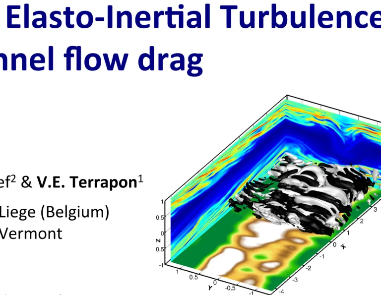
The role of elasto-inertial turbulence on channel flow drag

(1)

Role of Elasto-Iner/al Turbulence

on channel ﬂow drag

16th_{European Turbulence Conference 2017}

S. Sid1_, Y. Dubief2_{& V.E. Terrapon}1 1_{University of Liege (Belgium)}

2_{University of Vermont}

Figure 1 – Visualization of flow structures in three-dimensional flows. Contours of polymer elongation tr (C) /L2 in vertical planes, contours of streamwise shear fluctuations in a near-wall horizontal plane and turbulent structures identified by large positive (white) and negative (black) Q-criterion values. Left : Wi⌧ = 40, right : Wi⌧ = 100.

(2)

Elasto-Iner/al Turbulence • Non-laminar chaoLc state • Elas/c and iner/al instabiliLes EIT

Polymers and turbulence

2 Re Lam in ar Tu rb ul en t Elas/c turbulence Drag reduc/on • 2D • Small-scale cri/cal

(3)

! MDR Laminar Turbulent Newtonian ViscoelasLc 103 ₁₀4 10-3 10-2 Re_H f

Fric/on factor

–

_Simula/ons

3 Channel ﬂow (FENE-P)

Dubief et al. (Phys. Fluids, 2013) Terrapon et al. (J. Turbul., 2014)

Departure from laminar state at subcriLcal Re

(4)

Fric/on factor

–

_Experiments

4

Pipe ﬂow with 500 ppm PAAm solu/on

Samanta et al. (PNAS, 2013) 103 10-2 Re_D f MDR Turbulent Perturbed Unperturbed 10-3 104 Laminar SimulaLons and experiments agree

(5)

Numerical methodology

5 U_b H=2h x y z L_x+_{= 720} L_z+_{= 255} • DNS with FENE-P model • Periodic channel flow (const. pressure gradient) • 2D (512×128) and 3D (256×128×128) • IniLal perturba/on (blowing and sucLon at walls) • 2 different codes with different numerics

(6)

FENE-P model

6 ConLnuity Momentum Polymer stress ConformaLon tensor T = 1 Wi C 1− trC L2 − I " # $ % & ' ∂C ∂t + (u ⋅ ∇)C = ∇u ⋅ C + C ⋅ ∇u T − T ∂u ∂t + (u ⋅ ∇)u = −∇p + β Re ∇ 2 u +1− β Re ∇ ⋅ T + dP dx ex ∇ ⋅ u = 0 RaLo of solvent viscosity to zero-shear viscosity β = 0.97 Maximum polymer extension L = 70.9 Reynolds number Re+_{= 85} Weissenberg number Wi+_{= 40, 100} Xi & Graham (JFM, 2010) Similar results at lower Re+

(7)

Advec/on and small scales

7

∂C

∂t

+ (u ⋅ ∇)C = ∇u ⋅ C + C ⋅ ∇u

T

− T

AdvecLon Nonlinear source term Local ar/ficial diffusion (LAD) • Only locally applied • Never needed at low Re B • No diffusion • Hyperbolic • Sub-Kolmogorov scales • Need stabilizaLon Global ar/ficial diffusion (GAD) • Used by many with Sc_num ~ 1 • But Sc_polymer ~ 106 A

+

1 ReSc

∇

2

_C

⎡

⎣

⎢

⎤

⎦

⎥

GAD

(8)

Figure 1 – Visualization of flow structures in three-dimensional flows. Contours of polymer elongation tr (C) /L2 in vertical planes, contours of streamwise shear fluctuations in a near-wall horizontal plane and turbulent structures identified by large positive (white) and negative (black) Q-criterion values. Left : Wi_⌧ = 40, right : Wi_⌧ = 100. 1

3D simula/on at supercri/cal Re

8 Q-criterion Some spanwise homogeneity Wi+_{= 40} Polymer extension 0 1 Streamwise shear -10 10

(9)

3D simula/on at supercri/cal Re

9 Streamwise shear Q-criterion Structures are more 2D due to lower relaLve contribuLon of inerLa Wi+_{= 100} Polymer extension 0 1 Streamwise shear -10 10

(10)

2D simula/on at subcri/cal Re

10 Polymer extension Wi+_{= 100} Wi+_{= 40} C/L2 0 1

(11)

2D simula/on at subcri/cal Re

11 Streamwise velocity ﬂuctua/ons u_x′ / U_b 0.06 -0.06 Wi+_{= 40}

(12)

PIV measurements in viscoelas/c pipe ﬂow

12 Streamwise velocity ﬂuctua/ons at Re_D = 3150 0 20 30 50 100 150 Co nc en tr aL on [p pm ]

(13)

2D simula/on at subcri/cal Re

13 Fric/on coeﬃcient

10

100 1000

Re

_b

0.01

0.1 C

f

Newtonian

Wi=100, L=100

12/Re

_b

12.46/Re

_b0.96 101 ₁₀2 10-2 10-1 Re_H C_f 103 Viscoelas/c (Wi+_{= 100,}_L_{= 100)} ⇒ _C_f_{≈ 12.46 / Re}_H0.96 Newtonian ⇒_C_f_{= 12 / Re}_H Departure from laminar ﬂow similar to 3D

(14)

10 1 100 101 10 7 10 5 10 3 10 1 101 kx⌘K Ek 10 1 100 101 10 7 10 5 10 3 10 1 101 kx⌘K Ep

Figure 1 – Streamwise spectra of kinetic and elastic energies E_k and E_p averaged over the computa-tional and over time for di↵erent Schmidt numbers, Wi_⌧ = 40. Sc = 9, Sc = 16, Sc = 25, Sc = 100

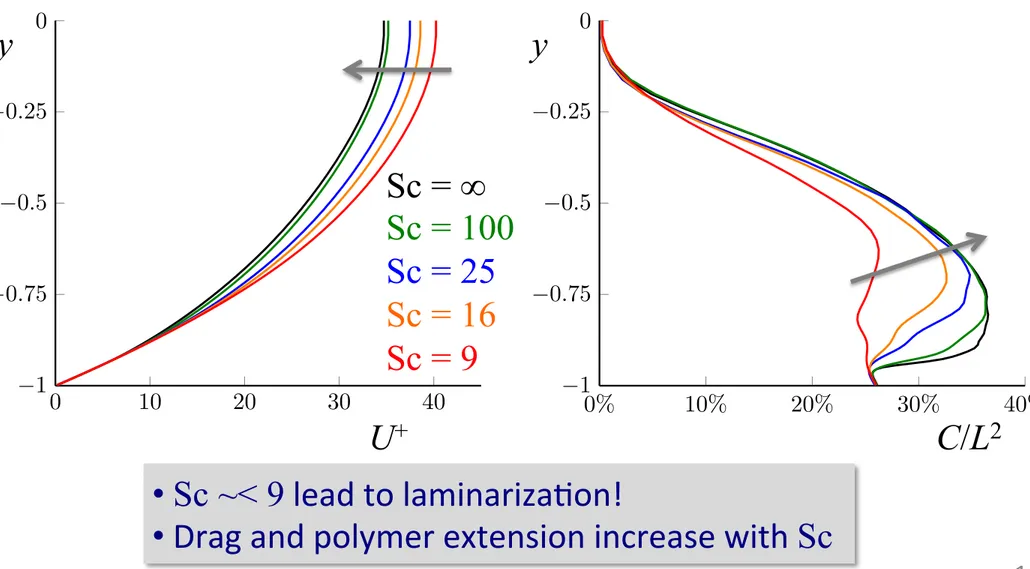
and Sc =_1. 0 10 20 30 40 1 0.75 0.5 0.25 0 U /u⌧ y/ 0% 10% 20% 30% 40% 1 0.75 0.5 0.25 0 tr C /L2 y/

Figure 2 – Left : Mean streamwise velocity profile, right : mean polymer elongation profile for di↵erent Schmidt numbers, Wi⌧ = 40. Sc = 9, Sc = 16, Sc = 25, Sc = 100 and Sc = 1.

1

Schmidt number eﬀect

14 Mean velocity Mean polymer extension y U+ _C/L2 y Sc = ∞ Sc = 100 Sc = 25 Sc = 16 Sc = 9 2D, Wi+_{= 40} • Sc ~< 9 lead to laminarizaLon! • Drag and polymer extension increase with Sc

(15)

Integrated streamwise spectrum of kine/c energy

15 10 2 10 1 100 101 10 7 10 5 10 3 10 1 101 ⌘K Ek 10 2 10 1 100 101 10 7 10 5 10 3 10 1 101 ⌘K E_p

Figure 1 – Streamwise spectra of kinetic and elastic energies E_k and E_p averaged over the

computa-tional and over time for di↵erent Schmidt numbers, Wi_⌧ = 40. Sc = 9, Sc = 16, Sc = 25, Sc = 100

and Sc = _1. 1 ⟨Φ_x(E_k+)⟩_y,t κ_xη_K Sc = ∞ Sc = 100 Sc = 25 Sc = 16 Sc = 9 Energy content at all scales increases with Sc 2D, Wi+_{= 40}

(16)

Integrated streamwise spectrum of kine/c energy

16 10 2 10 1 100 101 10 8 10 6 10 4 10 2 100 102 ⌘_K k,x

Figure 1 – Streamwise spectra of kinetic energy Ek for Re⌧ = 85. Gray dotted - 3D Newtonian, 3D Wi⌧ = 40, 3D Wi⌧ = 100 and 2D Wi⌧ = 40. 1 3D, Newtonian 3D, Wi+_{= 40} 3D, Wi+_{= 100} 2D, Wi+_{= 40} ⟨Φ_x(E_k+)⟩_yz,t κ_xη_K • 3D at lower Wi shows Newtonian features • 3D at larger Wi similar to 2D (less inerLal contribuLon) Re+_{= 85, Sc = ∞}

(17)

Conclusions

17 • EIT is mostly 2D • Small scales are criLcal • Need to respect physics (high Schmidt number) Open ques/ons • EIT = elasLc turbulence? • EIT = ulLmate MDR state? • Theory (predicLons, shape of spectra, …)

(18)

Acknowledgement

(19)

Ques/ons

(20)

BACKUP

(21)

Schmidt number eﬀect

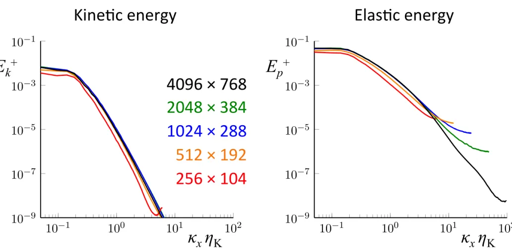
21 Time-averaged streamwise spectra KineLc energy ElasLc energy 10 1 100 101 10 7 10 5 10 3 10 1 101 kx⌘K Ek 10 1 100 101 10 7 10 5 10 3 10 1 101 kx⌘K Ep

Figure 1 – Streamwise spectra of kinetic and elastic energies Ek and Ep averaged over the

computa-tional and over time for di↵erent Schmidt numbers, Wi⌧ = 40. Sc = 9, Sc = 16, Sc = 25, Sc = 100

and Sc =_1. 0 10 20 30 40 1 0.75 0.5 0.25 0 U /u⌧ y/ 0% 10% 20% 30% 40% 1 0.75 0.5 0.25 0 tr C /L2 y/

Figure 2 – Left : Mean streamwise velocity profile, right : mean polymer elongation profile for di↵erent Schmidt numbers, Wi_⌧ = 40. Sc = 9, Sc = 16, Sc = 25, Sc = 100 and Sc = _1.

1 E_k+ _E p+ κ_xη_K κ_xη_K Sc = ∞ Sc = 100 Sc = 25 Sc = 16 Sc = 9 Wi+_{= 40} Small scales are criLcal!

(22)

Schmidt number eﬀect

22 Turbulent kine/c energy 0 10 20 30 40 0 0.04 0.08 0.12 tu⌧/ k 0 avg (t )

Figure 1 – Time series of the volume averaged instantaneous turbulent kinetic energy k_avg0 (t) for di↵erent Schmidt numbers. Sc = 6, Sc = 25, Sc = 50, Sc = 100.

1 k+ t+ Sc=25 Sc=6 Sc=50 Sc=100 Suﬃciently high Schmidt number is required to sustain EIT Laminariza/on Wi+_{= 310, Re}+_{= 40, β = 0.97, L = 70.9, GAD}

(23)

Schmidt number eﬀect

23 Ra/o of Kolmogorov (ν3_/ε)1/4 _{to viscous length scale (ν/u} τ) Wi+_{= 40, Re}+_{= 85, β = 0.97, L = 70.9, LAD} Kolmogorov larger than viscous length scale 9 16 25 100 1 3.5 4 4.5 5 5.5 Sc 1 ⌫ ⌘K

Figure 1 – Relative size of the Kolmogorov scale ⌘K = ⌫3/✏ 1/4 compared to the viscous scale ⌫ = ⌫/u⌧ for the Re⌧ = 85, Wi⌧ = 40 flow conditions.

1 η_K/ δ_ν

(24)

Sc=100

–

Inﬂuence of the mesh

24 256 ⇥104 512 ⇥192 1024 ⇥288 2048 ⇥384 4096 ⇥768 4 4.5 5 5.5 6 ·10 2 kavg 0.08 0.1 0.12 0.14 0.16 ⇤0_avg

Figure 1 – Mesh convergence analysis for the Re⌧ = 40, Wi⌧ = 310, Sc = 100 flow conditions. Mean

turbulent kinetic energy kavg (dark gray bars, plain line, left y axis) and mean polymer elongation

root mean square fluctuations ⇤0avg (light gray bars, dashed line, right y axis) averaged over the

computational domain for di↵erent spatial resolutions.

1 256 × 104 512 × 192 1024 × 288 2048 × 384 4096 × 768 Tu rb ul en t k in eL c en er gy Po ly m er e xte ns io n ﬂu ctu aL on s

Batchelor scale η_B = (Re+₎-1_Sc-1/2_captured

(25)

Sc=100

–

Inﬂuence of the mesh

25 Wi+_{= 310, Re}+_{= 40, β = 0.97, L = 70.9, GAD} Time-averaged streamwise spectra KineLc energy ElasLc energy E_k+ _E p+ 10 1 100 101 102 10 9 10 7 10 5 10 3 10 1 kx⌘K Ek 10 1 100 101 102 10 9 10 7 10 5 10 3 10 1 kx⌘K Ep

Figure 1 – Wall-normal and time-averaged stream-wise kinetic and elastic energies spectra Ek and Ep

for the Re⌧ = 40, Wi⌧ = 310, Sc = 100 flow conditions on 256⇥104, 512⇥192, 1024⇥288, 2048⇥384

and 4096_{⇥768 meshes. Wavenumbers are pre-multiplied by the computed Kolmogorov defined as} ⌘K = ⌫3/h✏i 1/4. 1 κ_xη_K κ_xη_K 4096 × 768 2048 × 384 1024 × 288 512 × 192 256 × 104

(26)

GAD vs. LAD

26 Wi+_{= 310, Re}+_{= 40, β = 0.97, L = 70.9, GAD / LAD} Time-averaged streamwise spectra KineLc energy ElasLc energy 10 1 100 101 102 10 9 10 7 10 5 10 3 10 1 kx⌘K Ek 10 1 100 101 102 10 9 10 7 10 5 10 3 10 1 kx⌘K Ep

Figure 1 – Wall-normal and time-averaged stream-wise kinetic and elastic energies spectra Ek and

Ep for the Re⌧ = 40, Wi⌧ = 310, Sc = 1 flow conditions on 1024⇥288 and 2048⇥384 meshes. The

black curve is the one obtained for Sc = 100 on the 4096_{⇥768 mesh. Wavenumbers are pre-multiplied} by the computed Kolmogorov defined as ⌘K = ⌫3/h✏i 1/4.

1 E_k+ _E p+ κ_xη_K κ_xη_K Sc = ∞ 1024 × 288 Sc = ∞ 2048 × 384 Sc = 100 4096 × 768

(27)

Code comparison

27 Wi+_{= 40, Re}+_{= 85, β = 0.97, L = 70.9, LAD} Mean velocity Mean polymer extension 0 10 20 30 40 1 0.75 0.5 0.25 0 U /u⌧ y/ 0% 10% 20% 30% 40% 1 0.75 0.5 0.25 0 tr C /L2 y/

Figure 1 – Left : Mean streamwise velocity profile, right : mean polymer elongation profile. Code A, 1024_{⇥288 ;} Code B, 512_⇥128. 1 y U+ _C/L2 Code A 1024 × 288 Code B 512 × 128 y

(28)

Transfer from kine/c to elas/c energy

28 y/η_K 0 25 Sc = 9 0 25 Sc = 16 0 25 Sc = 25 Sc = 100 0 25 Sc = ∞ κ_xη_K 10-1 ₁ 0 25 Flow ⇒ Polymers Polymers ⇒ Flow 0 28 -28

The role of elasto-inertial turbulence on channel flow drag

Role of Elasto-Iner/al Turbulence

on channel ﬂow drag

Polymers and turbulence

Fric/on factor

–

Simula/ons

Fric/on factor

–

Experiments

Numerical methodology

FENE-P model

Advec/on and small scales

∂C

∂t

+ (u ⋅ ∇)C = ∇u ⋅ C + C ⋅ ∇u

− T

+

1

ReSc

∇

C

⎡

⎣

⎢

⎤

⎦

⎥

3D simula/on at supercri/cal Re

3D simula/on at supercri/cal Re

2D simula/on at subcri/cal Re

2D simula/on at subcri/cal Re

PIV measurements in viscoelas/c pipe ﬂow

2D simula/on at subcri/cal Re

10

100

1000

Re

0.01

0.1

C

Newtonian

Wi=100, L=100

12/Re

12.46/Re

Schmidt number eﬀect

Integrated streamwise spectrum of kine/c energy

Integrated streamwise spectrum of kine/c energy

Conclusions

Acknowledgement

Ques/ons

BACKUP

Schmidt number eﬀect

Schmidt number eﬀect

Schmidt number eﬀect

Sc=100

–

Inﬂuence of the mesh

Sc=100

–

Inﬂuence of the mesh

GAD vs. LAD

Code comparison

Transfer from kine/c to elas/c energy

Φ

1−

β

Re

T

S

⎛

⎝

⎜

⎞

⎠

⎟

2D simula/on at subcri/cal Re

_Simula/ons

_Experiments

_C