Complex Potential and its Effects on Bound States

(1)

Complex potential and its effects on bound states

This article has been downloaded from IOPscience. Please scroll down to see the full text article. 1995 Phys. Scr. 51 146

(http://iopscience.iop.org/1402-4896/51/2/004)

Download details:

IP Address: 139.165.107.21

The article was downloaded on 05/12/2011 at 16:11

Please note that terms and conditions apply.

View the table of contents for this issue, or go to the journal homepage for more

(2)

Physica Scripta. Vol. 51, 146-153, 1995

Complex Potential and its Effects on Bound States

J. Cugnon and P.-B. Gossiaux

Universite de Liege, Institut de Physique au Sart Tilman, Bitiment B.5, B-4000 LIEGE 1, Belgium

Received January 10,1994; in revised form June 20,1994; accepted August 25,1994

Abstract

The coupling of bound states in a single-particle effective Hamiltonian through the addition of a negative definite imaginary potential is studied, both in a stationary and in a time-dependent formalism. Corresponding physical cases where this coupling is relevant are exhibited. Properties of the imaginary coupling matrix in the representation of the eigenstates of the real Hamiltonian are investigated. Consequences of these properties on the level widths and level shifts are exhibited on the two level case. Non trivial results, like forbidden values of the widths and level attraction are underlined. The conditions for the validity of the weak coupling approximation are examined. In the time-dependent problem, the typical time evolution patterns are illustrated both in the two level case and in the more realistic case of charmonium decay. When the initial state is an eigenstate of the real part of the Hamiltonian, it is shown that mixing of decay modes and quantum interference arise as consequences of the non diagonal imaginary coupling. Finally, the non locality of the imaginary potential corresponding to a diagonal imaginary coupling matrix in the state representation is also briefly studied and illustrated.

1. Introduction

It is very common in the non relativistic quantum mechani- cal description of two-body scattering or of the widths of (quasi) bounds states, to account for the loss of flux or of probability, due to the neglect of an explicit treatment of some channels, by means of an optical model potential with an imaginary part. A very popular example is provided by

the description of the elastic scattering of hadrons by nuclei, using an optical model with a complex potential, the imaginary part of which coming from the loss of flux due to the coupling to inelastic channels [l]. It is customary to analyse the data with a local imaginary potential, in spite of the fact that it can be shown on very theoretical grounds [2, 31 that the optical model potential is (weakly) non local and energy dependent. We will consider this optical model, namely the addition of an imaginary part to an effective one-body Hamiltonian, for bound states. We will be a little bit more general than usual, requiring the imaginary potential to be negative definite, allowing it to be local or non local. This model is usually studied, for stationary problems, by solving the static Schrodinger equation in r-space. When dealing with time-dependent problems, one would rather be tempted to work in the basis of the eigenstates of the real part of the Hamiltonian, at least when these eigenstates are easily constructed (like in the Coulomb case). Indeed, the problem then arises to solve a set of first order differential equations (instead of solving the time-dependent Schrod- inger equation in r-space, which is a parabolic partial differential equation). What we want to do here is to exhibit the relationship between the two descriptions (in r-space and in the state representation) and, in particular, to study the

Physica Scripta 5i

properties of the coupling imaginary matrix (in the state representation) corresponding to a negative definite imaginary potential. We want also to investigate briefly the consequences of these properties on those of the bound states, both in a stationary and a time-dependent picture.

2. Schrodinger equation in configuration space and in state

To be specific, we start with the time-dependent Schrodinger equation

representation

x d3r’W(r, r’)$(r’, t ) ,

where W(r, r’) is positive definite. We here restrict the dis- cussion to (quasi) bound states. This framework applies to many problems in hadron physics as well as in atomic physics. For instance, eq. (2.1) is appropriate to describe the evolution of a K - meson [4] or a K - meson

[SI

bound to a

nucleus in a Coulomb orbit, W (in general local in these cases) accounting then for the possible absorption of the meson due to strong interactions. A similar description is applicable to an antiproton bound by Coulomb forces to a nucleus, and to the protonium system [6]. Still another case

corresponds to the charmonium system where V(r) is the quark-antiquark potential and a local W stands for the coupling to the D-D channels [7, 81. In atomic physics, some aspects of the evolution of autoionization states [9] can be handled by eq. (2.1).

Instead of solving eq. (2.1) in r-space, one may be tempted to use a representation based on the stationary eigenstates of the real part, H,, of the Hamiltonian contained in eq. (2.1):

Assuming that the stationary eigenstates form a complete set, eq. (2.1) is then equivalent to the following set of equations

(3)

Complex Potential and its Effects on Bound States 147 Searching for stationary states of Hamiltonian (2.1)

would, in this representation, amount to solve the eigenvalue problem

j

We want to address to ourselves the following questions: (a) what are the general properties of the quantities wkj, corresponding to a negative definite, imaginary potential in r-space?; (b) what are the conditions for using the so-called weak coupling formula, corresponding to the neglect of the off-diagonal elements of wkj ?; (c) can one derive analytical

formula from the strong coupling case, at least in simple situations?; (d) what is the effect of the matrix W k j on the characteristic time evolution of the coefficients C k ( t ) , defined

in eq. (2.3)?

To make our motivation clearer, we do not pretend here to analyze all the physical effects linked with the imaginary part, as the underlying physical problem amounts to diago- nalize a Hamiltonian with a real coupling in a larger space, but we rather want to investigate primarily the mathematical properties of the eigenvalue problem (2.5), which, as we said, is often encountered in physics, because the many channel problem is often intractable. In particular, we want to point out the conditions that the quantities wkj should

satisfy and that one should enforce if one intended to mod- elize the coupling by eq. (2.5) from the very beginning, requiring however that this corresponds to the physical situation of a local negative definite imaginary potential. Never- theless, we will also point out some physical consequences

of

the imaginary coupling.

We will also pay some attention to the somehow reverse problem. Assume that in the basis of the functions $ k defined in (2.2), the absorption is diagonal, i.e. that one has the following set of equations, for the stationary problem (one may easily generalize to the time-dependent problem).

where the E,‘s are real. Translated into r-space, this equa- tion writes

A

+

V ( r )

I S

$(U) - i W(r, r’)$(r’) d3r’ = E$@), (2.7) with

In other words, if the “absorption is diagonal” in the state representation, it is in general non local in r-space. We will investigate the following questions : (a) what are the general properties of the quantity W(v, r’) defined by eq. (2.8)?; (b)

what would be the conditions for this quantity to be local or

almost local?

3. Properties of the quantities Wki

If the potential W(r, r‘) is given, the quantities wkjcan be calculated easily. However, it is worthwhile to find out the properties of the matrix wkj. This may be helpful in cases where one would like to use the optical model in the formu- lation (2.5) from the beginning and where the imaginary

part is not known in full detail and thus has to be postu- lated.

We consider (semi) positive definite W(r, r’)’, i.e. functions

which satisfy

d3r d3r’$*(r)W(r, r‘)$(r‘) 2 0,

s s

for any $(r), because it leads to a decrease of the norm of the wave function $(r, t ) in eq. (2.1), or to complex eigenvalues of the energy with negative imaginary parts in the stationary Schrodinger equation. For a positive definite operator, the matrix representing this operator in any basis is also positive definite [lo]. Therefore, all the principal minors are positive definite [ l l ] :

y j

2 0, (3.2)

yj

wkk-

wzj

>

0, (3.3) (3.4) q jwkk wl

+

yk

wkl

c“;i

+

yl

wkj &k - wj Wkk wj1-

wk,

4,

q ‘ j

-

w1

y’k wkj2 0,

. . .

Let us remark that the sufficient condition for wkj t o be positive definite is that the leading principal minor (i.e. the one in the upper left corner) of any rank is positive.

If W is positive definite and local, i.e. if W(v, r’) = W(r)G(v, r’), condition (3.3) can also be obtained from Schwarz’s inequality for integrals with a weighted norm [12]. Indeed, any matrix element wkj is a scalar product of $ k by $ j with the positive weight W(r). In this case, additional relations

may be derived. One has %k

k

(3.5) which proceeds from the invariance of the trace (let us recall that a local operator in configuration space has an infinite trace). One also has

as the wave functions $ k can be taken real, and

1

w;j =

I

$ k ( r ) W 2 ( r ) $ k ( r ) d3r, j i r (3.7a) W z j

<

max W 2 ( r ) , (3.7b) (3.8a) (3.8b) Relation (3.8a) can be obtained by the double commutator technique [13] or progenitor technique [14], which generate energy weighted sum rules, of which (3.8a) is just an example. In that particular case, it is easy to show that the 1.h.s. of (3.8a) is simply

i

The expressions below are written for a semi-positive definite operator

W , although we will not repeat the prefix “semi”. Of course, for a truly

positive operator the symbol “larger or equal” should be replaced by the symbol “larger”.

( E j - E k ) W i j = t < $ k

I

LW?

[IH,

3

wll

1

$ k ) . (3.9)

(4)

148 J . Cugnon and P.-B. Gossiaux 0 . 8 0 . 6 0 . 4 0 . 2 0 0.3 0 . 2 0.1 0 0 . 0 8 0 . 0 6 0 . 0 4 0 . 0 2 0 I I I 1

-I

L = 2 b L = b

-

0 5 1 0 1 5 2 0 2 5 3 0

i

Fig. 1. Variation of the quantities Wkj (eq. (4.3)) with the index j, for three values of L/b. In each case, the curves correspond to k = 1,3,5,7,9 and 11, successively, from the inner most one to the outer most one. The quantities

Wkj are displayed for odd values of j only (see text).

Performing the calculation of the double commutator and using

h

b,

W W l = T (VW),

1

(3.10) one readily obtains relation (3.8). One can in this way generate other relations similar to (3.7a) and (3.8a) with any posi- tive power of ( E j

-

Ek). Let us mention that the “energy weighted sum rules” are obtained here for a real local poten- tial, V(r). They can be generalized for non local V and non local W but then they imply more complicated forms of the r.h.s. of relation (3.8a) and similar ones.

In the case of a bounded local function W ( r ) (which occurs in many physical cases), relation (3.6) sets bound on the values of the diagonal matrix elements, whereas relations (3.3), (3.7) and (3.8) set bounds on the off-diagonal matrix elements and on the variations of the quantities wkj with their indices k and j . This means that the diagonal ele- ments of wkj are all bounded and that the off-diagonal elements are constrained by eqs. (3.3), (3.4), and should decrease, when one goes farther and farther off the diagonal, sufficiently fast for the summations (3.7) and (3.8) (or their generalizations) to converge.

Of course, all the conditions (3.2)-(3.4) for non local imaginary parts and (3.2)-(3.8) for local imaginary parts are not sufficient to determine the matrix wkj, but they have to be Physica Scripta 51

fulfilled if one wants the matrix W k j to correspond to a positive definite operator.

4. Illustrative cases

To give an idea of the typical variation of W , with its indices, we have calculated the matrix elements in two simple but illustrative cases. The first one corresponds to V being an infinite square well in one dimension (-

R,

<

x

<

R,)

and W being a step function, i.e. W ( x ) = WO 8(L

-

I

x I).

One then obtains ( L

-=

R,)

sin

[E

( k - j ) ]

+

sin

[”

RO

( k

+

j

+

1 )

Wkj =

-

X k - j k + j + l

for the positive parity states ( k , j = 0,

1,2,

. .

.), and [sin

[E

( k

-

j ) ] sin

[E

( k

+

j ) ] ]

(4.2) wkj=

-

n k - j k + j

for the negative parity states ( k , j = 1, 2, 3,

. .

.). If k = j , the first term in the parenthesis of both eq. (4.1) and (4.2) should be replaced by zL/R,. Relation (4.2) also applies to the three-dimensional case for 1 = 0 waves.

The second case corresponds to the harmonic oscillator in one dimension, V = i m o 2 x 2 and W ( x ) =

WOe-X2’L2.

One then obtains

1 - k - j . a2

x 2F1( - k , - j ; (4.3)

where 2F1 is the hypergeometric function and where a’ =

i(1

+

b2/L2), b being the oscillator characteristic length:

b =

d m .

Formula (4.3) applies when k

+

j is even, otherwise wkj vanishes.

For the square well, the quantities wkj decrease slowly, when departing from the diagonal ( k = j ) , i.e. when k is fixed and j ( > k ) increases, oscillating between a maximum, behaving as l / j as j increases, and a minimum of opposite sign. It is remarkable that this behaviour is barely sufficient to ensure the convergence of the summation in (3.7a). For the harmonic oscillator, when k is fixed and j is increasing, wkjdecreases as

(4.4) the quantity in parenthesis always being smaller than unity. The quantities (4.3) are displayed in Fig. 1. These examples illustrate the fact that the elements of the matrix W k j are decreasing when going further and further apart from the diagonal, as eq. (3.7a) implies. They also suggest that the large j behaviour (for fixed k ) depends upon the ranges of the real and imaginary potentials.

5. Weak and strong imaginary couplings

5.1. Introduction

In many cases of physical interest [4-61, one usually calcu- lates the eigenfunctions

Jlj

by solving the Schrodinger equa- tion for the real part of the Hamiltonian H , (see eq. (2.2)) in

(5)

Complex Potential and its Effects on Bound States 149 r-space and the widths of the bound states are very often

calculated by using the popular weak coupling formula

When Schwarz’s inequality is violated, p is negative. The eigenvalues are given by

It is very hard to discuss the validity of this formula in all generality. It is better to look at this problem whex it is formulated in state representation (eq. (2.3) and (2.4)), since then the weak coupling approximation amounts to neglect- ing the off-diagonal matrix elements of the matrix wkj. Of course, some difficulties appear with this representation. One is inevitably led to truncate the (in principle) infinite matrix wkj, for practical reasons. The size of the matrix which would correspond to the same accuracy as the stan- dard techniques of solving Schrodinger equation in r-space, is presumably very large. Therefore, it is certainly hopeless to investigate the effect of the off-diagonal elements in all generality. In our opinion, it is, however, worthwhile to study the two level case first. This may appear to be only academic, since it would be very exceptional if the dynamics would decouple two of the + j states from the rest. Neverthe- less, we believe that some features of the two level case, that we outline below, may persist in some form in the general problem, and that may help us to study the validity of the weak coupling, both in the static and the time-dependent cases.

5.2. The static two level case

The eigenvalue problem (2.5) takes then the simple form (El

’

E2)

-iW12 E, - -iw12 E - iW2,

)(;:)

= 0 (5.2) E,

-

E

-

iW,,

(

As we explained in section 3, if we want the model defined in eq. (2.5) to correspond to a negative definite imaginary absorption, the quantities wkj are bound to fulfill some constraints. In the two level case (eq. (5.2)), these constraints reduce to the non negativity of W,, and Schwarz’s inequality

(5.6) The advantage of expression (5.6) is the fact that criterion (5.3) enters through the p parameter only: hence, x - , y and

p can be varied independently, provided one restricts to positive values of p .

Let us first concentrate on the widths r k , i.e. minus twice the imaginary parts of the eigenvalues

=

{(J-

+

p )

2

Im ,/(I

-

ix-l2 - y2}.

r1,2

IE, - E2I

(5.7)

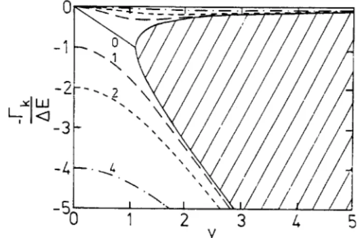
The typical variations of the widths with respect to the parameters y and x - (corresponding to the difference of W,, and W22) are given in Fig. 2, for p = 0, i.e. for the maximum non diagonal coupling just fulfilling requirement (5.3). The remarkable result is the forbidden region indicated by the shaded area, It is easy to trace back the mathematical origin of this forbidden region. Let us consider x - = 0, for simpli- city. The square root in (5.7) has no imaginary part as far as

y2

<

1: in that particular case, the two widths are identical and are represented by the diagonal in Fig. 2. As soon as y is larger than unity, the two eigenvalues start to differ. Figure 2 tells that, whatever the value of x - , when the coupling (y) becomes too strong, one of the imaginary parts grows at the expanse of a decrease of the other. The forbidden region is thus an intrinsic property of the complex coupling.

When one allows for a departure from p = 0, but in con- cordance with Schwarz’s inequality, i.e. p > 0, the pattern does not change. There is a mere shift of the curves towards the bottom of Fig. 2, i.e. a uniform increase of the imaginary parts. When Schwarz’s inequality is violated, p

<

0, the curves in Fig. 2 are shifted to the top and at least one of the

w:2 4 1w22 2 (5.3)

which requires the non negativity of W2,

.

It is convenient to express the quantities in terms of reduced parameters

Wll - w22 Wll

+

w22 El - E2 El - E 2 ’ , x - = El

+

E2 E = - E, - E,’ x + = (5.4) y=- 2w12 El - E , ’ The parameter p = x , - J W (5.5a)

Y

expresses the conformity to Schwarz’s Indeed? it _{Fig, 2. Level widths (divided by L\E}₌_{E , -}_{E 2 )}_{for the}_two _level _and can be rewritten as _for_p₌_{0 (the maximum coupling compatible with Schwarz’s inequality), as}

function of the parameters y and x - , whose values are indicated close to

1 _{the corresponding curves. Note that for}_{x -}_#_{0, there are two curves, rep-} resented by the same symbol. For x- = 0 (full curves) the two curves coalesce up to y = 1 and diverge for higher values. The shaded area indi- cates the forbidden values of the widths.

W l l

+

W22)

p = -

El - E 2

(6)

150 J . Cugnon and P.-B. Gossiaux

imaginary parts can become positive. Therefore, in the two level case, Schwarz's inequality is equivalent to a sufficient criterion for having absorption only and not creation of flux, whatever the values of the parameters, as we explained in Section 3.

The role of Schwarz's inequality (or more generally of conditions (3.2)-(3.4),

. .

.) is thus rather clear. Would one wish to study the coupling of bound states in H , with other channels by model (2.5) from the very beginning, arbitrary values of the matrix W k j are not permitted. In the two level case, only those consistent with Schwarz's inequality (and of course with the positive definiteness of W,, and W2J would lead to the same physics as a negative definite imaginary potential, i.e. to pure absorption.

The introduction of the parameter p is very convenient to exhibit the consequences of Schwarz's inequality, but for the subsequent discussion, it is preferable to stick with the parameters x , , x - and y. The widths are then given by

= x , Im J(1

-

ix-j2 - y 2 . (5.8)

l-1. 2 ( E , - E21

They are represented in Fig. 3, which actually displays the 1.h.s. of eq. (5.8) after subtraction of x ,

,

i.e. the average of W,, and W,, , divided by E , - E , (see eq. (5.4)). The for- bidden zone in this representation is also visible. The limi- tations imposed by Schwarz's inequality take the form y

<

,,

6-,

i.e. restrict the allowed values of y, for fixed x , and x-

.

It can be checked that, under these conditions, the quantities

T i

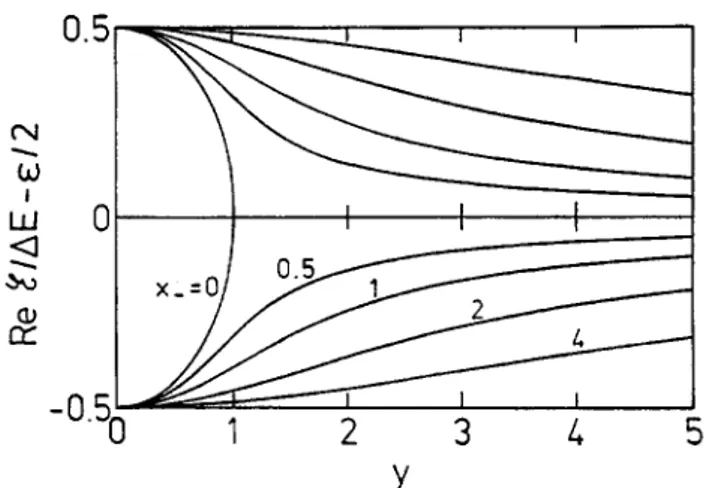
are positive.

Let us say a few words on the real parts of the complex eigenvalues. They are given by

( E & Re J(1 - ix-I2

-

Y,}, _(5.9) E , - E2 Re

L?,,

= ~ 2 or E ,

+

E2 Re

L?,,

-

=

*$

Re J(1 - ix-)2

-

y 2 . (5.10) 2 El

-

E2

They are thus symmetric with respect to ( E ,

+

E 2 ) / 2 . The numerical values are given in Fig. 4. The most remarkable result is that the imaginary coupling introduces an attrac-

i

0 1 2 3 4 5

Y

Fig. 3. Level widths (divided by AE = E , - E , prior subtraction of x+), as functions of the parameters y and x- , whose values are indicated. The exact values of the widths (eq. (5.8)) are given by the full curves, while the dotted curves correspond to approximation (5.1 1).

Physica Scripta SI

0.5

N

w

\ I

0 .n

3u

-"'"O

1

2

3

4

5 Y

Fig. 4. Real part of the eigenvalues for the two level case (with respect to the mean value of the unperturbed energies, see eq. (5.9b)), as functions of the parameters y and x- , whose value is indicated close to the corresponding curve. For x- = 0 and y > 1, the two real parts are vanishing.

tion of the eigenvalues, in contrast with the real coupling case which produces a repulsion of the eigenvalues [l5]. For

x - = 0, i.e. for W,, = W,, , the two eigenvalues coalesce for y

>

1 (the quantity (5.9b) then vanishes). For x- # 0, they almost coalesce for large values of y.

In summary, we found the following non trivial behaviour of the eigenvalues: ( i ) the real parts are pulled toward one another by the imaginary coupling (level attraction); (ii)

these are forbidden regions for the imaginary parts of the eigenvalues, whose consequence is the growth of one of the imaginary parts at the expanse of the other when the imaginary coupling is increased. It is more appropriate to say that there are strictly forbidden values of the difference of the widths at strong coupling, as illustrated by Figs 2 and 3.

We conjecture that these results hold qualitatively in the general (many level) case. Indeed, property ( i ) holds for an imaginary coupling of any strength. It is opposite to the result for real coupling case and it is well known that level repulsion occurs in the many-level case, giving rise to a larger dispersion of the eigenstates. We emphasize that the level attraction linked to the imaginary coupling should be viewed as a mathematical property. In an actual physical case, when the underlying full many-channel problem is solved with a real coupling, only level repulsion occurs. However, when the full problem is reduced to the equivalent one-channel problem with a complex coupling, the real part of the coupling would lead to a too strong level repulsion, which would be corrected by the level attraction due to the imaginary coupling. Property (ii) is a genuine property of the imaginary coupling. If this property holds for the many- level case, it may lead in the strong coupling case to a strong increase of one or a few widths. We have verified (see below) on a specific case that the properties of the decay of

an eigenstate of the real part of the Hamiltonian (mode mixing) are still valid on a more general case. The correlated decrease of the remaining widths should be reflected by an enhancement of the small width part of the width distribution in a small energy interval. This is embodied by the so- called Porter-Thomas distribution for the widths [ 161, and verified experimentally [17]. As far as we know, the possible link between the results of the above two state model and the Porter-Thomas distribution has never been discussed or alluded to.

(7)

Complex Potential and its EfSects on Bound States 151 - 8 - N 0 -

-

h * - 2 - U” M 0

-

- 4 -

-

‘ 1 0 - - 0 . 5 -

-

1- - 1 . 5 - 5.3. W e a k coupling

As we said above, we are interested in knowing under which conditions the widths can be accurately estimated by the first order (in the diagonal coupling) formula (5.1). It is very hard to answer this question in all generality with argu- ments based on perturbation theory. Indeed, the next order approximation to

rk

in terms of the non diagonal matrix elements wkj (i.e. including the diagonal elements in the

unperturbed energies), is given by y I- 0.2 2

f

, \

I (5.11)

and therefore implies complicated properties of the

wkj’s

and of the unperturbed spectrum. The two level case can thus be of some help to illustrate the situation when a level is perturbed by its very near neighbors only.

In the two level case, approximation (5.1 1) corresponds to the first order approximation in y2 in eq. (5.8), keeping x,

and x - fixed, while approximation (5.1) corresponds to

y = 0. Approximation (5.11) is compared to the exact result in Fig. 3. It is quite accurate up to y = 2W12/(E1-E2)

5

0.5, irrespective of the value of x- and surprisingly good for larger values of the coupling y, when x- is large. Note however the complete failure for x- = 0 and y

>

1, where

the problem becomes suddenly non perturbative.

The second term in (5.1 1) gives also an idea of the accu- racy of the weak coupling approximation (5.1). In the two level case, it is equal to x- yz/l

+

( x - ) ~ ) . It is interesting to note that for a given value of y2, this term is small when x-

is either very small or very large, and is the largest for x- = 1.

From the last result, it may be expected that the first cor- rection to (5.1), i.e. the second term in eq. (5,11), may be considered as providing an accurate result, as far as the equivalent of the y parameter for the many level case is

6

0.5. We propose the following straightforward extension of the y parameter

(5.12)

In summary, one expects that when the last quantity is

5

0.5, expression (5.1 1) is quite accurate.

5.4. Time-dependent problem

We want here to investigate the time evolution of the wave function $(r, t ) (eq. (2.1)) when one starts at t = 0 with an eigenstate of Ho (eq. (2.2)), or equivalently the time evolu- tion of the coefficients ck(t) (eq. (2.3)) when, at t = 0, all of them vanish but one, which is equal to unity.

Let us first start with the two level case, with c1 (t = 0) = 1 and c2 ( t = 0) = 0. As we explained in section

5.2, the two relevant parameters are x- and y. So we illustrate the typical behaviours of

I

c1

l 2

and

I

c2

1’

for various values of the parameters x- and y in Fig. 5. They can be understood when one notices that the general solution of eq.

(2.3) can be written as ( h = 1)

(5.13)

(::I

and

(::)

where q , are the complex eigenvalues (5.6),

are the corresponding eigenvectors and where al and a2 are

0 1 2 3 4 5 t (fdc) x- = 0.2 0 4 8 1 2 1 6 t (fdc) I

F i g . 5. Time evolution of the 1 ci(t)

(*

(eq. (5.13)) for various values of the

parameters x- and y (and p = 0) in the two level case. Note the different vertical scales and the different time scale for the upper left part of the figure, indicated at the top of the figure.

standing to guarantee the initial conditions. Therefore, one has

I

c , ( t )

I2

=

I

a1

l 2

I

d , I2eWr1‘

+

I

a 2

I2

I

b , 12e-r2f

+ 2 R~ (Cr*ld* 1 2b 1, i R e ( b i - 8 z ) r e - ( r i + r z )t/2). (5.14)

Note that one has a , d l

+

a 2 b l = 1. The variation of

I

c l ( t )

I z

shows the two exponential decays due to the first two terms in eq. (5.14), plus oscillations (of quantum nature) due to the last term in eq. (5.14) which are damped rapidly if the widths are sufficiently large. The oscillations are the most impor- tant when y

5

1 and x - is close to zero. One can see that in all cases, the quantity

I

c,(t)

1’

decreases exponentially by several orders of magnitude before changing of slope, except for very strong coupling. Therefore, the strong coupling does not only change the imaginary parts of the eigenvalues (compared to simplest approximation (5.1)), but also intro- duces a rapid turn-over from one decay mode to the other one. Let us notice that in the weak coupling approximation

(5.1),

1

c l ( t )

l 2

is purely exponential and c2(t) vanishes.

In Fig. 6, we illustrate the behaviour of the

1

ci(t)

1’

for a more realistic problem: the charmonium model of Ref. [7]. The potential V ( r ) is the usual charmonium potential and

W ( r ) is taken as a constant value, W O , for r > l.0fm and zero below, reflecting the idea that a quark-antiquark string breaks into a D-D system, if the length is long enough. At

t = 0, the system is supposed to be in the so-called $‘2) state,

and then evolves under the imaginary coupling. Equation

(2.1) is solved with a very large mesh in r-space (step size z 0.01 fm), which amounts to solve (after appropriate projection yielding the coefficients ci(t)) eq. (2.3) in a very large basis. When the coupling is small, the initial state decays exponentially several orders of magnitude before a change of slope takes place. When the coupling is strong, the various modes are mixed more rapidly. It is remarkable

(8)

152 J . Cugnon and P.-B. Gossiaux

1 0 '

order to reproduce a diagonal imaginary coupling matrix. They are: 1 0 ' U

-

h 1 0 " .c, v

-

U

-

1 0 ' 1 0 " WO I 200 M e V WO I 200 M e V

'

3

-! 2 1

r

nnr nnr' R , 4n rr R , R , W ( r , r') =

-

1 <

sin

-

sin

-.

t (fm/c)

Fig. 6. Time evolution of the quantities I tit) l2 for the case of the charmonium system (see text and Ref. [7]), for various values of the imaginary coupling parameter W O .

that the typical behaviours observed in the two level case are reproduced in this realistic case. If one considers the two states $ ( 2 ) and $' only, the cases illustrated by the central

and bottom part of Fig. 6 correspond to x - = 0.23 and

y = 0.39 and to x - = 0.58 and y = 0.98, respectively. There

is indeed a strong resemblance, as far as the variation of the quantity

I

c i ( t )

l 2

is concerned, with respectively the upper and central parts of Fig. 5 (second column), for which the values of the coefficients x - and y are similar. Let us finally mention that the first value of the imaginary strength,

W O ,

is the closest to the actual physical value [7].

6. Properties of W(r, r') associated with a diagonal

In this section, we make some remarks on the (reverse) problem stated in the end of section 2. Let the effective

bound state problem be expressed by eq. (2.6) in the representation of the eigenstates of the real one-body Hamilto- nian. We first here list the main properties of the corresponding imaginary potential (see also eqs. (2.7) and (2.8)),

imaginary coupling matrix

to be added to the real part of the one-body Hamiltonian, in

Physica Scripta 51

(1) W(r, r') = W(r', r), W(r, r) 2 0.

( 2 )

1

W(r, r ) d3r =

-

1

1 Tj.

2 3

This results from the invariance of the trace of an operator. 1 ( 3 )

1

[W(r,

r')12

d3r' =

-

1 rf

t+bf(r). ( 4 )

11

[W(r,

r')I2

d2r d3r' =

-

1 rf

.

(6.4) (6.5) 4 , 1 4 ,

The latter proceeds from the invariance of the norm.

( 5 ) [W(r, r')12

<

W(r, r)W(r', r'). (6.6)

This is a consequence of Cauchy's inequality [lo].

These conditions are resting on the positivity of the Tis.

Other properties are related with the variations of the Tj's

with the indicesj. Indeed, if all the Tis are equal, W(r, r') is diagonal. Of course, this also depends upon the eigenfunctions

+,.

So a general discussion is out of scope. We illustrate the non locality of W (r, r') in the case of a three- dimensional infinite square well of radius R , for I = 0 waves. The corresponding multipole of W(r, r') writes

Introducing the coordinates R = (r

+

r')/2, s = r

-

r', (with 0

<

R

<

R , , 0

<

s

<

2R,), one obtains

m

x

1

I-"[ cos

(T)

.

-

cos

)I

(:

(6.8)

n = 1

Let us consider the three following cases:

( 1 )

r n

=

r/n.

One then has:

In this case, W(r, r') is infinite for r = r', but rapidly decreases as s increases, like

(6.10) ( 2 )

r n

= I-/n2. One can then write

W ( r , r') = - 1 7

r

[x

n 2 R -

-

n 2 R 2

- -

n21sI

+ E ] .

R i 2R0 4 R i

4nR0 R 2 - 5 4

(6.1 1) In this case, W(r, r') is finite for r = r' as it should when

E,

Tj converges (see eq. (6.2)), and for small s, the behaviour is the following

(9)

Complex Potential and its Efects on Bound States 153 (3)

r,

= T/n4. One has, in this case,

1 I- W(r, r’) =

-

S2 R 2 - - 4nR0 4 ~ [ ~ ( l - - ~ ~ - - $ $ ( l - - ~ ) ~ ] . n4R2 (6.13)

The behaviour for small s is given by

s2R: W(r, I ) )

-

1 -

4RZ(R0 - R)’ *

(6.14) One sees that the form of the non locality (i.e. the formal analytic dependence upon s for small s) is changing with the exponent of n in the three cases mentioned above. It can be

proved that the quadratic dependence on s survives for all powers larger or equal to 4. This formal dependence is also

the one which is phenomenologically considered (see Ref. [ l]), as a gaussian form in s is often used.

It is also interesting to consider the case

r,

= Tu”, with

a

e

1. One then obtains

1

r

W(r, r’) = -

-

S2 R2

_ -

4nR0 4 2nR

1

1 - a cos

(e)

1 - a cos

(z)

-

1

-

2a cos

(z)

+

a2 1 - 2a cos

(e)

+

a2

RO

(6.15) For small s, one obtains the following behaviour

The usual quadratic dependence with a negative coefficient is also obtained. Furthermore, the last expression clearly indicates that the faster

r n

decreases when n + CO (i.e. for

smaller and smaller values of a), the larger is the non locality.

7. Conclusion

We have studied the complex coupling between bound states in an effective one particle Hamiltonian. This situation is often encountered in physics, when a many channel problem cannot be solved and when the approach is restricted to a one channel problem with an effective inter- action. We studied this problem when the coupling occurs through a negative definite imaginary potential. We have exhibited the properties of the corresponding imaginary matrix when the problem is formulated in the representation

of the eigenstates of the real part of the Hamiltonian.

We have studied the simple but illuminating two level case and underlined the importance of Schwarz’s inequality which constrains the value of the non diagonal coupling in the state representation. Non trivial results, as level attraction and excluded values for the difference of the widths have been worked out.

We have also delineated for the two level case the accuracy of the weak coupling approximation (5.1) to the widths (in the first order of the diagonal coupling, i.e. in zeroth order in the off-diagonal coupling). It is surprisingly good in a large domain of the (x-, y ) parameter plane, especially for largely different diagonal elements (large x -). Furthermore, the first correction to (5.1), i.e. the second term in (5.11), gives a good approximation to the exact result in a wider range of the ( x -

,

y ) plane. We proposed a qualitative criterion for a general situation.

We also investigated the time evolution of an eigenstate of the real Hamiltonian in the presence of the imaginary coupling. We have shown that decay mode mixing and quantum interferences are consequences of the imaginary coupling, and disappear in the limit of weak coupling. We displayed in one physical case, the interplay of several decay modes.

Finally, we investigated the properties of the imaginary potential in r-space, corresponding to a diagonal imaginary matrix in the state representation. We derived a qualitative relation between the variation of the elements of the matrix

and the non locality of the corresponding imaginary potential.

Acknowledgements

This work was supported by contract SPPS-IT/SC/29 and by the FNRS, Belgium. References 1. 2. 3. 4. 5. 6. 7. 8. 9. 10. 11. 12. 13. 14. 15. 16. 17.

Hodgson, P. E., “Nuclear Reactions and Nuclear Structure”, (Clarendon Press, Oxford, 1971).

Feshbach, H., Ann. Phys. (N.Y.) 5,357 (1958); 19,287 (1962). Mahaux, C. and Weidenmuller, H. A., “Shell-model Theory of Nuclear Reactions” (North-Holland, Amsterdam, 1969).

Hufner, J., Phys. Rep. 21, l(1975).

Batty, C. J., Sov. J. Part. Nucl. 13, 71 (1982). Batty, C. J., Rep. Prog. Phys. 52, 1165 (1989).

Cugnon, J. and Gossiaux, P.-B., Europhys. Lett. 20, 31 (1992). Cugnon, J. and Gossiaux, P.-B., Z. Physik C58, 77 (1993). Fano, U., Phys. Rev. 124, 1866 (1961).

Schiff, L. J., Quantum Mechanics, 3rd ed., (McGraw-Hill, Tokyo, 1968), ch. 6.

Hohn, F. E., “Elementary Matrix Algebra”, 3rd ed., (The Macmillan Company, New York, 1973), ch. 10.

Abramowitz, M. and Stegun, I. A., “Handbook of Mathematical Functions”, (Dover, New York, 1972), p. 11.

Lane, A. M., ”Nuclear Theory”, (Benjamin, New York, 1964). Noble, J. V., Ann. Phys. (N.Y.), 67, 98 (1971); Phys. Rep. C40, 241 (1978).

Wigner, E. P., Proc. Conf. on Neutron Physics by Time-of-Flight, Gatlinburg, Oak Ridge National Report ORNL-2309 (1956). Porter, C. and Thomas, R. G., Nucl. Phys. 104,483 (1956).

Lynn, J. E., “The Theory of Neutron Resonances Reactions”, (Clarendon Press, Oxford, 1968), ch. 6.