A tool to design steel elements submitted to compartment fires—OZone V2.
Part 1: pre- and post-flashover compartment fire model
J-F. Cadorin, J-M. Franssen
Département de Mécanique des Matériaux and Structures, Université de Liège, Bât. B52I3, Chemins des Chevreuils, 1, 4000 Liège, Belgium Abstract
The computer code OZone V2 has been developed to help engineers in designing structural elements submitted to compartment fires. The code is based on several recent developments, in compartment fire modelling on one hand and on the effect of localised fires on structures on the other hand. It includes a single compartment fire model that combines a two-zone model and a one-zone model.
In this paper, the description of this compartment fire model is given. The main model is first presented. It consists of the usual zone model equations fully coupled with the partition model equations. The partitions are modelled by the finite element method. The switch from the two-zone to the one-zone model is then explained. The vertical, horizontal and forced vent sub-models are presented, followed by the fire source and the
combustion models. A comparison between this code and another compartment fire model NAT is made. The OZone calculations are then compared to full scale fire tests.
Considerations as to how this model is used for the design of steel elements will be presented in a companion paper (Fire Saf. J., this issue).
Keywords: Compartment fire; Zone model; Partition model; Tests Nomenclature
1ZM one-zone model
2ZM two-zone model
y the ratio of specific heat (dimensionless)
ρj density of the material of the finite element j (kg/m3)
ρg gas density (1ZM) (kg/m
3
)
ρU and ρL gas densities of, respectively, the upper (U) and lower (L) layer (2ZM) (kg/m3) ξox concentration of oxygen in the gas inside the compartment (dimension-less)
εp relative emissivity of partition-gas interface (dimensionless) σ constant of Stefan-Boltzman (5.67 x 10⁻⁸) (dimensionless)
Ai,vv,cl area of the closed opening (m2) Af floor area of a compartment (m2) Afi horizontal burning area of fuel (m2)
Afi,max maximum horizontal burning area of fuel (m 2
)
Ap total area of partitions of the compartment (excluding openings) (m2)
Ap,j,i total area of partitions j connected to the zone i (m2)
At total area of partitions of the compartment (including openings) (m2) Av total area of vertical opening (m
2
)
AVjj area of vertical opening no. j connected to the zone i (m2)
b width of vertical vent (m)
C capacity matrix of partition (W/K s m2) Cel,j capacity matrix of finite element j (W/K s m
2
)
Cd discharge coefficient (dimensionless)
cj specific heat of the material of the finite element j (J/kg K)
cv(T) specific heat of the gas in the compartment at constant volume (J/kgK)
Cp(T) specific heat of the gas in the compartment at constant pressure (J/kgK)
D fire diameter (m)
E1ZM(ts) total energy in the two-zone model system (Eg + energy in partitions) (J)
E2ZM(ts) total energy in the two-zone model system (EU + EL + energy in partitions) (J)
Eg internal energy (1ZM) (J)
EU and EL internal energies of, respectively, the upper and lower layer (2ZM) (J);
gel,j load vector of finite element j (W/m2) h convective heat transfer coefficient (W/mK)
H height of the compartment (m)
Hc,net complete combustion heat of fuel (obtained in bomb calorimeter) (J/kg) Hc,eff effective combustion heat of fuel (in real fire) (J/kg)
m combustion efficiency factor (dimensionless)
kj conductivity of the material of the finite element j (W/K s m2)
conductivity matrix of finite element j (W/K s m2) conductivity matrix of partition (W/K s m2)
length of finite element j (m)
rate of mass entrainment in the fire plume (kg/s) pyrolysis rate (kg/s)
pyrolysis rate defined in the data (kg/s) total mass of fuel in the compartment (kg) mass of the gas in the compartment (1ZM) (kg)
mass of oxygen in the compartment (kg)
mass of oxygen in the compartment at initial time (kg)
mass of oxygen coming into the compartment through vents (kg) mass of oxygen going out of the compartment through vents (kg) and mass of the gas of, respectively, the upper and lower layer (2ZM) (kg)
rate of mass of gas exchange through vent, i = U or L or g. β = in or out. α = VV or HV or FV (kg/s). number of equations for the ceiling (dimensionless)
number of equations for the floor (dimensionless) number of equations for the wall no. j (dimensionless)
number of equations for all the partitions (dimensionless) absolute pressure in the compartment considered as a whole (Pa).
convective part of the heat release rate (W) radiative part of the heat release rate (W)
characteristic fire load density per unit floor area of compartment (J/m2) design fire load density per unit floor area of compartment (J/m2)
energy radiated from the fire per unit area of lower layer partition (W/m2) energy content of the zone i, i = U or L or g (J).
energy exchange through vent, i= U or L or g.β = in or out. α = VV or HV or FV (W). energy exchange between partitions and zone i (i = U or L or g) (W/m2)
energy radiated from the fire per unit lower layer partition area (kg/s) the universal gas constant (dimensionless)
rate of heat release (W)
rate of heat release defined in the data (W)
rate of heat release per unit floor area of compartment (W/m2) time of switch from the 2ZM to the 1ZM (s) temperature (K)
vector of node temperature of finite element j (K) temperature of the gas (1ZM) (K)
temperature of the gas outside the compartment (K) vector of node temperature of partition (K)
temperature of node j (K)
and temperatures of the gas of, respectively, the upper and lower layer (2ZM) (K) volume of the compartment (constant) (m3)
rate of volume of gas through a forced vent (m3)
and volumes of, respectively, the upper and lower layer (2ZM) (m3) height of a forced vent (m)
height of neutral plane (m) fuel height (m)
zone interface height (m)
height of the sill of a vertical vent (m) height of the soffit of a vertical vent (m)
Subscripts
c variable related to convective heat transfer ce variable related to the ceiling
f variable related to the floor area fi variable related to the fire source FV variable related to the forced vent g variable related to the single zone of \ZM HV variable related to the horizontal vent
i equal to U for variable related to upper layer, to L for variable related to lower layer and to g for variable related to the single zone of 1ZM in variable added to a compartment zone
L variable related to the lower layer
out variable subtracted from a compartment zone p variable related to partitions
pj variable related to partitions no. j r variable related to radiative heat transfer U variable related to the upper layer VV variable related to the vertical vent w variable related to the wall
1. INTRODUCTION
Zone models are numerical tools commonly used to evaluate the development of the temperature of the gases within a compartment during the course of a fire. Based on a limited number of hypotheses, they are easy to use and provide a good evaluation of the situation provided they are used within their real field of application. Different developments of numerical fire modelling have appeared since the first zone models were proposed [1-3], including multi-compartment and computational field dynamics models. Although single compartment zone models are the least sophisticated among numerical fire models, they have their own field of application and are an essential tool in fire safety engineering practical applications.
The main hypothesis in zone models is that the compartment is divided into zones where each zone has a uniform temperature distribution at any time. In single-zone models, the temperature is considered to be uniform in the whole compartment. This type of model is thus usually used in the case of fully developed fires. In two-zone models, there is a hot gas layer which is close to the ceiling and a cold gas layer which is close to the floor. Two-zone models are thus normally used in case of localised fires or during the pre-flashover phase.
The aim of this paper is to present a new compartment fire model called "OZone V2" and to show a comparison between its results and full scale fire tests.
This code includes a two-zone and a single-zone model with the ability to switch from the two-zone to the one-zone model if some criteria are encountered. It thus deals with localised and fully developed fires. The wall model is based on the finite element method and is fully coupled to the zone equations. Different combustion models have been developed to cover different situations of use of the code, i.e. test simulations or design situations.
A comparison of the one-zone model of OZone and another one-zone model NAT [6], from CSTB, France, has been made. A comparison has also been made between OZone simulations and 36 tests performed at CTICM, France [7].
2. OVERVIEW OF THE COMPARTMENT MODEL AND OF ITS BASIC ASSUMPTIONS
The aim of this section is to give an overview of the main assumptions on which the different models and sub-models included in OZone are based and to explain the heat and mass transfer in the compartment model. The formulations of the main model and of the sub-models are given in the next sections.
• a two-zone model (compartment and partitions); • a one-zone model (compartment and partitions);
• a model to switch from the two-zone to the one-zone model.
Some sub-models are connected to the main model. Sub-models enable the evaluation of:
• the heat and mass transfer between the inside of the compartment and the ambient external environment through vertical, horizontal and forced vents (vent model).
• the heat and mass produced by the fire (combustion model);
• the mass transfer from the lower to the upper layer by the fire plume (air entrainment model);
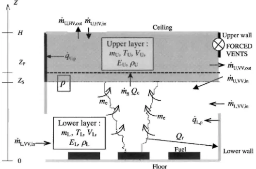
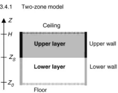
Fig. 1 shows a schematic view of the zone model and its sub-models for heat and mass transfer. In the two-zone model, the compartment is divided into an upper and a lower layer. In each layers the gas properties (temperature, density, etc.) are assumed to be uniform. The pressure is assumed to be constant throughout the whole compartment volume (except when evaluated mass exchange through vents).
The layers are separated by an adiabatic horizontal plane (at height Zs). They are only connected by an air entrainment model. An air entrainment model is an empirical model which enables the estimation of the rate of mass entrained from the lower to the upper layer by buoyancy in the fire plume. The plume volume is not considered (no mass or heat balance is calculated on it). It is thus included in the lower layer volume. Fig. 1. Schematic view of two-zone model and associated sub-models.
The upper zone is supposed to be opaque and the upper layer partitions (wall and ceiling) are connected to it by radiative and convective heat transfers. The lower layer is clear and the lower layer partitions are connected to it by convective heat transfer only. Vertical partitions are thus divided into two parts, one in the lower layer and one in the upper layer. The height of the two parts is equal to the relative zone height. These heights are varying with time.
The fire is defined by its rate of mass loss, its rate of heat release (RHR) and its area. Qc is the convective part of
the RHR and Qr is the radiative part of the RHR. Qc is often in the range of 0.6-0.8 RHR [8] and has been fixed in
the code to 0.7 RHR. The radiative part is thus fixed to 0.3 RHR. In this model Qc is transmitted to the upper
layer and Qr to the lower layer partitions (through a source term in the lower layer partition formulation). In the
lower layer, the heat is thus transferred by radiation from the fire to the lower layer partitions and then transferred by convection from the partitions to the lower layer and by conduction within the partitions. Even if the lower layer is clear, the radiation between partitions is not evaluated because, on one hand,
temperatures of the different partitions are often quite low and similar, leading to low radiative heat flux between partitions, and, on the other hand, the radiative heat flux from the fire to the partitions should often be
Heat and mass transfer through horizontal, vertical and forced vents are exchanged with the layer at the same height, with some exceptions for incoming air through vertical vent which is always added to the lower layer and for forced vent close to the zone interface.
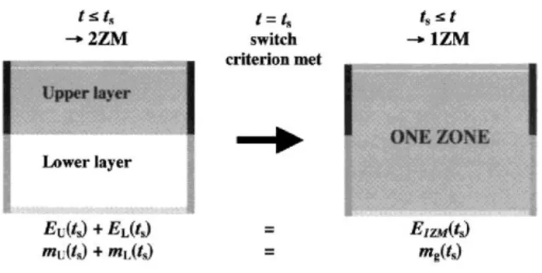
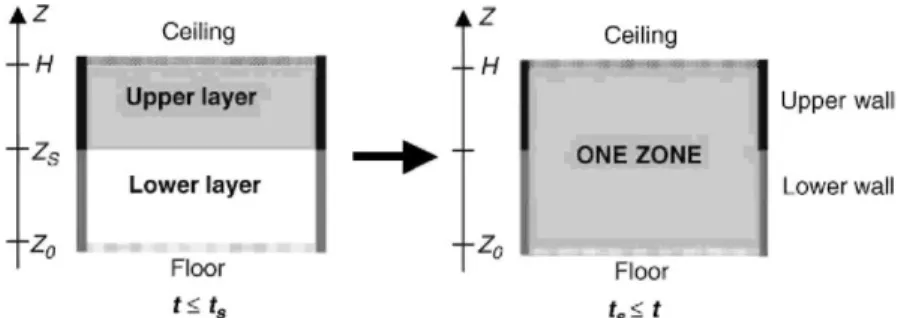
Some switch criteria are defined so that they represent a limit beyond which one-zone model assumptions becomes closer to the physics of the fire situation than the two-zone model ones. If during a two-zone model simulation, a switch criterion is met (time ts), the two-zone model is left and replaced by a one-zone model. The
switch is made so that the total energy and mass present in the 2ZM system at time of switch are fully conserved in the 1ZM system (Fig. 2).
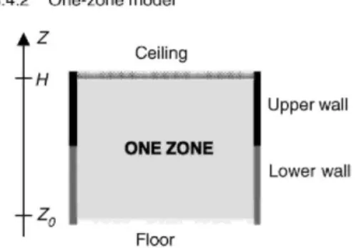
Fig. 3 shows a schematic view of the zone model and its sub-models for heat and mass transfer. In the one-zone model, the compartment is represented by a single one-zone. In this one-zone the temperature and density are assumed to be uniform. The pressure is assumed to be constant in the whole compartment volume (except while evaluating mass exchange through vents). The zone is supposed to be opaque and partitions are connected to it by radiative and convective heat transfers.
Fig. 2. Transition from 2ZM to 1ZM.
Fig. 3. Schematic view of one-zone model and associated sub-models.
The fire is defined by its rate of mass loss, its rate of heat release and its area. All mass and energy coming from the fire are added to the single zone.
Heat and mass transfer through horizontal, vertical and forced vents are exchanged with the single zone.
In 2ZM as well as in 1ZM, the fire is defined by a heat release rate, rate of mass loss and fire area curves function of time. These three curves have to be defined by the user. The input curves correspond to fuel controlled fire, i.e. to the fire which would occur without any influence of the compartment. These curves may be modified if the ventilation is limited (combustion models) or if the gas temperature is sufficiently high to ignite the fuel.
3. FORMULATION OF THE MAIN MODEL
The procedure usually presented in the literature sets the limits of the compartment on the inside surface of the wall and adds a partition sub-model on top of it. The proposed procedure amounts in fact to set the limit of the main model on the outside boundary of the compartment. The main model thus includes the zone(s) and the partitions. The equations describing the situation inside the compartment and in the partitions are solved simultaneously with an implicit procedure; the energy balance between the gas and the partition is totally respected. The finite element method is used to represent the partition and a particular formulation of it has enabled to couple it to the zone equations.
The flux at partition boundaries are dependent on the surface temperature of the partition. When using the finite difference method, the temperature is calculated in the middle of each element. A simple way to evaluate the surface temperature is to assume it to be equal to the temperature at the centre of the first element [9]. This latter assumption is only valid if elements are small. When using the finite element method, temperatures are evaluated at each node; the surface temperature is thus directly evaluated. This comment shows that the finite element method enables to discretise a partition with less (and thus bigger) elements than the finite difference method. With an explicit time integration procedure, the zone temperature calculated at time t is used to evaluate the partition temperatures at time t + At, and zone temperature at t + At is then evaluated. For one time step At used to evaluate zone temperature, five time steps may be needed to evaluate the partition temperatures. Some assumptions have to be made on the evolution of zone temperatures (constant, linear, etc.). Time steps with an explicit procedure have to be short enough to make this assumption valid [9]. On the other hand, it is well known that an implicit procedure enables the use of bigger time steps.
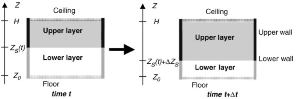
Partitions can be modelled by one-dimensional (1D) finite elements in the case of a single-zone model; on the other hand, partitions of the two-zone model should theoretically be modelled by 2D finite elements. One-dimensional finite elements used in case of 2ZM, lead to neglect the vertical fluxes in walls and to artificially create or remove some energy. The latter is because the thickness of both zones varies with time, thus changing the boundary conditions of a part of the wall. For instance, a part of wall that is initially connected to the lower layer may later become connected to the upper layer if the upper layer thickness increases.
Fig. 4. 2ZM and partition model at times t and t + ∆t.
Considering an increasing upper layer thickness during the time interval At (Fig. 4), a wall section of height ∆ZS
is transformed from lower wall to upper wall. As the temperatures in the lower wall are generally lower than those in the upper wall, some energy is thus artificially created here in the model. On the contrary if the upper layer thickness is decreasing, some energy is lost. The only way to be absolutely rigorous when modelling walls in 2ZM, would be to make a single 2D partition model which would take into account vertical fluxes and the variation of Zs in the boundary condition of the 2D elements.
A 1D partition model is nevertheless considered in OZone V2, for the two-zone as well as for the one-zone model. Preliminary work on a two-zone model with a 2D partition model [10] has indeed shown that the partition model based on 1D finite elements is a sufficiently good approximation of the reality; the difference of the gas temperature calculated with 1D or 2D partition model being of a few degrees only. In most cases, the 2D character of the heat transfer can be neglected. The increase in computing time and the significant difficulties encountered in defining the compartment are quite important if the walls are represented by 2D elements whereas it has a marginal effect on the results of principal interest, the zone temperatures and the zone thickness. Moreover, even in high compartment with small floor area for which the 2D effect may become more important, the error in neglecting it should be much smaller than one due to the assumption of uniform temperature in
zones.
3.1. Two-zone model
Numerical two-zone models are normally based on 11 physical variables. These variables are linked by seven constraints and four differential equations describing the mass and energy balances in each zone. The time integration of these differential equations gives the evolution of the variables describing the gas in each zone. The mass balance equation expresses the fact that, at any moment, the variation of the mass of the gas in a zone is equal to the sum of the mass of combustion products created by the fire plus the mass coming into the compartment through the vents and the mass going out of the compartment through the vents. The energy balance equation expresses the fact that, at any moment, there is a balance between the energy which is produced in the compartment by the combustion and the way in which this energy is consumed: by the heating of the gases in the compartment, by the mass loss of hot air through the openings (including a negative term accounting for the energy of incoming air), by the radiation loss through the openings and, finally, by the heating of the partitions. The term "partition" represents all the solid surfaces that enclose the compartment, namely the walls (vertical), floor and ceiling (horizontal).
The 11 variables which are considered to describe the gas in the compartment are: the mass of the gas of, respectively, the upper and lower layers, and ; the temperatures of the gas, and ; the volumes,
and ; the internal energies, and ; the gas densities, and , of respectively, the upper (U) and lower (L) layer; and finally, the absolute pressure in the compartment considered as a whole, p.
The seven constraints are:
The specific heat of the gas at constant volume, , and at constant pressure, , the universal gas constant, R, and the ratio of specific heat, , are related by
The variation of the specific heat of the gas with the temperature is taken into account by the following relation obtained by a linear regression on the tabulated data given in the SFPE Handbook of Fire Protection Engineering [11]:
The mass balance equations have the general form of Eqs. (4) and (5). A dotted variable means the derivative of
x with respect to time.
Four basic variables have to be chosen to solve the system. Provided that the zone temperatures, TU and TL,the
height of separation of zones, Zs and the difference of pressure from the initial time, are selected, Eqs. (4)-(7) can be transformed [12] into the following system of ordinary differential equations (ODE):
3.2. One-zone model
In the case of a one-zone model, the number of variables which describe the gas in the compartment as a whole is reduced to six: i.e. the mass of the gas, mg; the temperature of the gas, Tg; the volume of the compartment
(constant), V; the internal energy, Eg; the pressure in the compartment, p; the gas density, pg
The number of constraints is reduced to four:
Eq. (13) expresses the mass balance:
Eq. (14) expresses the energy balance:
Two basic variables have to be chosen to solve the system. Provided that the zone temperature, T, and the difference of pressure from the initial time, Ap, are chosen, Eqs. (13) and (14) can be transformed into the following system of ODE:
3.3. Partition model
A partition is discretised by a 1D finite element model as depicted in Fig. 5. With this discretisation, the temperature is computed at the interface between the different layers, or elements, and a linear temperature variation on the thickness of each element is assumed.
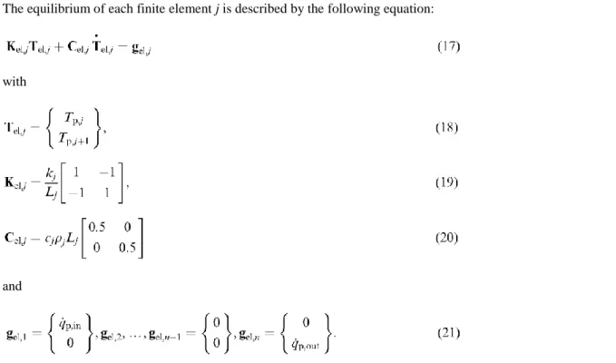
The equilibrium of each finite element j is described by the following equation:
with
and
Eqs. (19) and (20) are in fact simplified expressions because the material properties have been considered as constant in each element, thus taking them as constant multipliers of the matrix; the temperature dependency in the element could also be taken into account by Gauss integration techniques but it has not been done in this model. Eq. (20) is furthermore the diagonalised version of the true matrix. An advantage of the diagonal form is that it smoothes the spatial oscillations which could arise in the solution if too thick elements are used in the discretisation. Another advantage is related to the computing strategy, as will be explained in the formulation of Eq. (24).
The assembly of the n partition equations of type (17) that can be written for each of the N finite elements making the partition produce the system of Eqs. (22) in which the size of the vectors and the matrices are N + 1 and (N + 1) x (N + 1), respectively.
where
The energy transmitted at the partition interface results from heat transfer by convection and radiation between the zone and the partition and between the fire and the partition. The energy transmitted at the interface between the outside world and the partition is due to heat transfer by convection and radiation.
From the system of Eq. (22), it is easy to derive analytically the system of Eq. (24), owing to the diagonal nature of C.
This system of equations is a set of N differential equations for the N temperatures of the partition. The temperature of the compartment is only present in the first term of the load vector, see Eqs. (21), (23) and (26)-(29). The system has a similar form as the system of Eqs. (8)-(11) (2ZM) and of Eqs. (15) and (16) (1ZM) established for the variables of the gas zones.
3.4. Connection of the zones and the partitions equations
Partitions can be divided into three types: the ceiling, the floor and the walls. The basic finite element formulation is the same for the three types of partitions but the boundary conditions are different.
3.4.1. Two-zone model
In the 2ZM, the ceiling is always connected to the upper layer and the floor to the fire and to the lower layer. Vertical partitions are divided into two parts, an upper section, connected to the upper layer and a lower section connected to the fire and to the lower layer (Fig. 6). The area of each part is calculated by multiplying the length of the wall by its height. The height varies with time and is function of the height of separation of the zones, Zs. The area of the openings included in each partition is subtracted.
The finite element discretisation of the two parts are identical, only the boundary conditions are different. The system of Eq. (24) has to be constructed once for the ceiling, once for the floor and 2M times if the enclosure has M different types of walls. and are the number of nodes of the ceiling and of the floor, and is the number of nodes of the wall no. j. The partitions thus leads to differential equations:
For all types of partition, the energy transmitted at the interface between the external environment and the partition is due to heat transfer by convection and radiation:
The upper layer is composed of a mixture of combustion products and fresh air entrained by the plume from the lower layer. It is considered to be opaque and radiation between partitions connected to it are neglected. The
energy transmitted between the inside surfaces of upper partition and the upper layer results from heat transfer by convection and radiation:
The lower layer is composed essentially of fresh air with very little combustion products. It is thus considered as transparent. The energy exchanged between the inside surfaces of lower partitions and the lower layer results only from heat transfer by convection according to Eq. (28). Moreover the partition exchange heat with the fire by radiation, this term is represented by . The total heat exchange with partition is thus given by Eq. (29).
is obtained by dividing the radiative part of the rate of heat release Qr by the total area of lower partitions,
including the opening area and including the floor:
Fig. 6. 2ZM and partition model.
3.4.2. One-zone model
When considering a one-zone model during an entire simulation, a vertical partition is consisted of two parts connected to the single zone. The finite element discretisation of the two parts and the boundary conditions are identical. Therefore, the temperature distribution in the partitions and the flux densities on the boundaries are the same in the two parts. In a one-zone model a vertical wall would normally not be divided into two. The results obtained with two partitions for a single wall are identical to those with one single partition model. Having two partitions will increase the number of equations to be solved and therefore the computing time. This division in two parts is done in order to allow eventual combination of the 2ZM and \ZM as explained in Section 3.6 (Fig. 7).
The partitions lead to Neq,p differential equations, also given by Eq. (25).
3.5. Time integration
In a 2ZM, Eqs. (8)-(l 1) and Eq. (24) form a set of Neq,part + 4 differential equations which can be passed on to the
numerical solver. This solver will integrate the equations, taking into account the coupling between the compartment and the partition, and solving the Neq,part + 4 variables, which are the pressure variation, the
temperature in the upper zone, the temperature in the lower zone, the height of the zone interface and the temperatures at each node of the partitions.
The same procedure holds for a 1ZM with Eqs. (15) and (16) and Eq. (24) built Neq part times.
The system of ODE describing the situation is stiff. A physical, although not rigorous from a mathematical point of view, interpretation of stiffness is that the time constant relative to the pressure variation is much shorter than the time constant of the temperature variation. It is therefore usual to rely on a specialised library solver
specifically written for this kind of problem. In the code OZone, the solver DEBDF [13] is used. Fig. 7. IZM and partition model.
3.6. Switch from two-zone to one-zone model
If some criteria are encountered during a two-zone simulation, the code will automatically switch to a one-zone simulation, which better suits the situation inside the compartment at that moment. The simulation will continue until the end of the fire under the hypothesis of a one-zone model. The aim of this section is to show how the code deals with the basic variables of the zone models, how it sets the initial conditions of the one-zone model and how it deals with partition models. The criteria for switching are also listed. A complete description of the criteria and of their effect on the simulation process is given in [14].
3.6.1. Zone models formulation
ts is the time at which the switch from the 2ZM to the 1ZM occurs. The values of the 11 basic variables
describing the gas in the two zones are known at ts. To continue the simulation with a one-zone model, it is
possible to start solving Eqs. (15) and (16). The point is to set the 1ZM initial values.
In a one-zone model there are six variables describing the gas in the compartment as a whole, linked by four constraints. Two new constraints are thus needed to fix the new initial conditions.
These two additional conditions are obtained by setting that during the transition from two zone to one zone, the total mass and the total energy of gas in the compartment are conserved.
The initial one-zone temperature Tg(ts) and one-zone pressure p(ts) can be deduced from Eqs. (33), (34) and (12).
A consequence of this procedure is that Tg(ts) is lower than TU(ts) and higher than TL(TS)and thus the temperature
3.6.2. Wall model formulation
The partition temperatures, the height of the lower and upper walls (vertical partitions) Zs(ts) and H - Zs(ts) are
known at time ts. From ts to the end of the calculation, the one-zone model is linked to the lower and upper walls
which keep the dimension they had at time ts, i.e. Zs(ts) and H - Zs(ts). During the transition no modification of
partition temperatures or wall dimension is made; only the boundary conditions at the interface with the compartment are modified. This way to proceed enables to fully respect the conservation of energy during the transition from the two-zone to the one-zone model.
With a two-zone model, lower walls are heated directly by radiation from the fire, and they give back energy to the lower layer by convection. After the switch is encountered, these walls exchange energy by radiation and convection with the single zone (Fig. 8).
3.6.3. Ignition and switch criteria
The switch from 2ZM to \ZM is based on four criteria. Two criteria are linked to the ignition of the fuel and two others are related to the loss of validity of the two-zone assumption. While the first two criteria are related to a physical phenomenon which may occur during compartment fires, the last two are related to the limits of applicability of the two-zone model assumptions.
It is important to note that users have the possibility to activate or not any of these criteria and to decide on the value of the relevant parameter at which the criteria are met. The default value proposed here are only
informative and not necessarily applicable to any situation. 3.6.3.1. Flashover criterion.
A high temperature of the upper layer leads to a flashover. All the fuel in the compartment is ignited by radiative flux from the upper layer.
Fig. 8. Switch from two-zone to one-zone model.
In a recent overview of flashover studies [15], the upper layer temperature and the heat flux received by the fuel leading to flashover obtained in different experimental studies have been collected. The temperature values are included between 450° C and 800°C with most values between 600°C and 700°C. The heat flux values are between 15 and 33kW/m2. This shows the high level of pure uncertainty on the flashover phenomenon. Anyway, if the definition has to be unique, the most common value admitted to characterise flashover is 600° C which corresponds to a heat flux of about 20 kW.
In OZone, the default value of the upper layer temperature leading to flashover is 500°C. The temperatures between 600°C and 700°C given in the literature correspond to temperatures near the ceiling, while the upper layer temperature of a two-zone model is an average temperature on the upper layer volume and is therefore lower than the temperature near the ceiling.
3.6.3.2. Ignition criterion.
If the gases in contact with the fuel have a higher temperature than the ignition temperature of fuel, the
Babrauskas [16] reports that ignition temperature of wood exposed to the minimum heat flux possible for ignition is around 250°C. The surface temperature of fuel is usually used as an empirical parameter to describe the ignition of fuel. Nevertheless, it is particularly convenient to use the temperature of the environment to characterise ignition in compartment fire modelling because the environment temperature is the main result of such models. But even in test built-up for ignition temperature evaluation, the environment temperature is often used as a criterion.
Taking into account a difference between the surface and the surrounding environment temperatures, the default value of the zone temperature at which ignition occurs has been set in the code to 300°C.
3.6.3.3. Interface height criterion.
The interface height may go down and lead to a very small lower layer thickness, which is not representative of a two-zone phenomenon.
It seems difficult to have an upper layer fulfilling nearly all the compartment and to still consider the two-zone model assumptions. As an example, the heat transfer by radiation from the fire to the lower partitions should be overestimated if the lower layer is too thin, the radiant part of the flame being in most part included in the upper layer. Moreover numerical problems will be encountered for a very thin lower layer.
In the code, the default value of the interface height criterion is 20% of the compartment height. 3.6.3.4. Fire area criterion.
The fire area may be too big compared to the floor surface of the compartment to consider a localised fire. In this situation the volume of the plume itself may be quite big and the two-zone assumption ignores this fact.
For example, in an 8 x 8 m2 compartment, 25% of the area is covered by the fire if a square fire of 4 x 4m2 is in the centre of the room, which means that only a 2m wide "corridor" of non-burning floor surface is left between the fire and the walls. Models based on a localised fire should not be applied in this case. The hypothesis of a uniform temperature seems more likely to be a better representation.
In OZone, the default value of the fire area criterion is 25% of the floor compartment area. 4. EXCHANGES THROUGH THE VENTS
Three types of vent models have been introduced in OZone V2: vertical vents, horizontal vents and forced vents. Although the pressure is uniform in the compartment when solving the basic equations of the problem, the pressure is not uniform in the compartment when calculating the mass flow through the openings. In this case, the variation is exponential with the height.
4.1. Vertical vents
4.1.1. Conυectiυe exchanges
The mass flow through vents is calculated by integrating the Bernoulli law on each opening [17].
With A is the variable at origin of the flux, B the variable at destination of the flux, Z' and Z" are bounds of integration on height Z, i the U if the integration is made in the upper layer, L if the integration is made in the lower layer and g in case of one-zone model, β the in if gas goes in the compartment, out if gas goes out of the compartment, sign the (+1) if gas goes in the compartment, (-1) if gas goes out of the compartment.
If the height where the pressure inside the compartment is equal to the pressure outside of the compartment is in a vertical vent, the vertical vents is divided into two parts, one where the mass flow goes inside the compartment and another one where the mass flow goes outside. This height is called the neutral plane height. Moreover in
two-zone model, if the height of separation between the zone is in the opening, another subdivision is
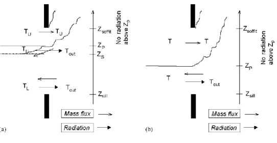
encountered. In 1ZM, three possibilities exist depending on the neutral level position. In 2ZM, 10 possibilities exist depending on the neutral level and the zone separation height positions. For each vertical vent, Eq. (35) is evaluated 1-3 times with the appropriate bounds of integration on the height (Z' and Z" can be the sill of the vent, the soffit of the vent, the neutral plane height or the separation between the zone height). Fig. 9 shows in case of
2ZM and IZM one possible situation of relative position of Zsill, ZP, Zs and Zsoffit∙
The energies contained in these mass fluxes are:
In the two-zone model, all the mass coming into the compartment through the vertical vent is added to the lower layer. This hypothesis has been made considering the fact that the gas coming in has a higher density than the gas inside and thus, due to buoyancy, goes downward when coming in (Fig. 9a).
Fig. 9. Exchanges through vertical vents in (a) 2ZM and (b) IZM.
4.1.2. Radiative exchanges
The radiation through vertical vents is taken into account by the Stefan-Boltzman law. It is considered that the radiation exists only below the height where the pressure inside the compartment is equal to the pressure outside the compartment. Above this level, the gases go out of the compartment and the temperature outside (in the plume) is assumed to be equal to the temperature in the compartment and thus it is considered that the net radiation flux is equal to zero (Fig. 9). This latter hypothesis may be too conservative when the outflow is very thin and not completely opaque. Nevertheless, this effect should only be significant for a large opening size.
If the opening is closed no mass exchange exists through it. The opening can either be assumed to be adiabatic and thus no radiation through it is considered or be assumed to be non-adiabatic and the radiation flux is evaluated by
Ai,VV,cl is the area of the closed opening. εgl is a parameter which includes the relative emissivities of the gases
and the part of energy which is reflected on the interfaces between gas and glass and absorbed by the glazing material.
4.2. Horizontal vents
Gas flow through a horizontal ceiling vent is not always driven by the single pressure difference, buoyancy can also have a significant effect. These forces may lead to bi-directional exchange flow through the vent. Therefore, it is not appropriate to unconditionally use Bernoulli's equation to model flow through horizontal vent.
Cooper has proposed a model and the associated FORTRAN subroutine for calculating flows through circular, shallow (i.e. small depth to diameter ratio), horizontal vents [18-20]. This model gives the flow considering the pressure-driven forces and when appropriate the combined pressure and buoyancy effects. This subroutine has been included in the code.
4.3. Forced vents
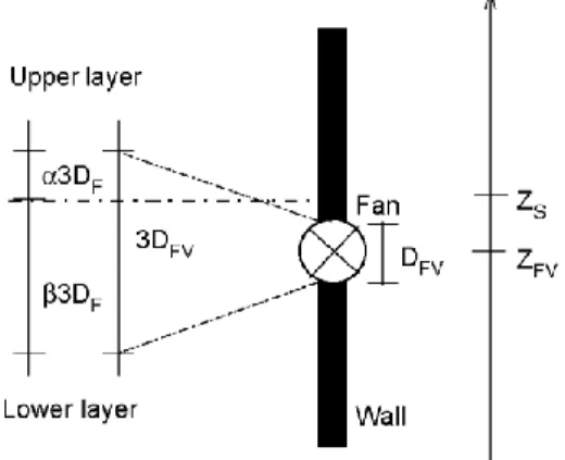
Forced vent model is built to represent the effect of mechanical ventilation. The forced vents are defined by the volume rate flow that they induced, , their height ZFV and their diameter DFV.
When the zone interface is above the forced vent elevation +1.5DFV, the exhausted gas is lower layer air only.
When the zone interface is below the forced vent elevation -1.5DFV) the exhausted gas is upper layer air only.
When the zone interface is between ZS + 1.5DFVand ZS -1.5DFV,the mass of extracted air from each layer is
given by a linear interpolation (Fig. 10).
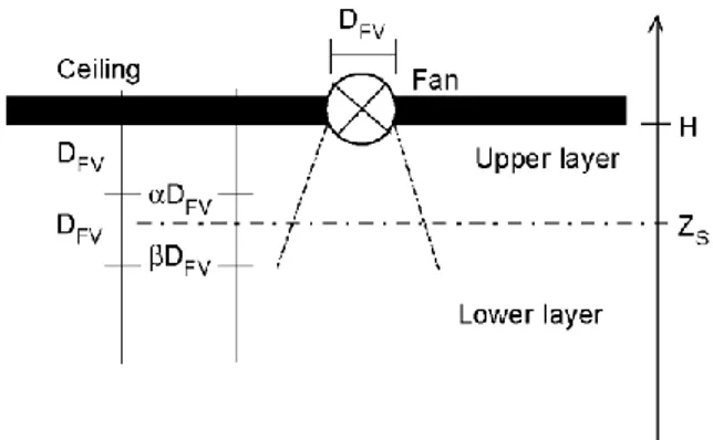
If the forced vent is in the ceiling the interpolation is made as shown in Fig. 11. When the zone interface is above the forced vent elevation -DFV,the exhausted gas is lower layer air only. When the zone interface is below the
forced vent elevation -2DFV,the exhausted gas is upper layer air only. When the zone interface is between ZS -
DFVand ZS - 2DFV,the mass of extracted air from each layer is by a linear interpolation (Fig. 11).
The latter procedure to decide whether the flow is exchanged with the upper or with the lower layer is based on the fact that the volume on which forced vent flow has an influence should depend, among other things, on the fan diameter. The bounds of the influence zone (3DFVand 2DFV)have been fixed arbitrarily. The parameter DFV
is only used in this definition of these bounds, thus, if a more precise knowledge of this phenomenon is known, it can be fixed to any value, not necessarily linked to the real dimension of the vent.
Moreover, in case of 2ZM, if the mass was extracted at a single height with the corresponding zone and if the mass extracted was bigger than the entrained mass in the plume, some numerical problems would be
encountered. The proposed procedure enables to avoid these numerical problems.
Fig. 11. Schematic view of forced vent model in the ceiling.
4.4. Opening size variation
During the course of a fire the number of vents that are open can vary. Their size can also be modified. This can be the result of glazing breakage, automatic opening or firefighter action, etc. In this code, the opened vent size can be defined to be a function of the temperature of the zone in contact with the glass or to be a function of time.
The size variation of a vertical vent is modelled by a variation of its width. The size variation of a horizontal vent is modelled by a variation of its area.
5. FIRE SOURCE—INPUT OF HEAT AND OF COMBUSTION PRODUCTS IN THE COMPARTMENT
To represent the fire, the basic inputs are the heat release rate RHR(t) (W), the pyrolysis rate (kg/s) and the fire area function of time. The pyrolysis rate is taken into account in mass balances and the heat release rate in energy balances. The fire area is used in some air entrainment models. This section explains the physical parameters used to define the fire source, how they are related and how OZone deals with them in function of the oxygen available in the compartment. The strategy of calculations may also influence these inputs as explained in [14].
5.1. Basic parameters
5.1.1. Heat release rate—RHR
The heat release rate is the quantity of energy that is released by the fire per second. The RHR depends on the type and quantity of fuel present in the compartment, on the quantity of oxygen available in the compartment, on phase of the fire (rising, stationary, decreasing), etc.
5.1.2. Heat release rate density—RHRF
The heat release rate density is the quantity of energy that is released by one square metre of fire per second.
5.1.3. Pyrolysis rate—
The pyrolysis rate is the quantity of mass of solid fuel that is transformed into combustible gases per second. It is indeed the mass loss rate of fuel.
5.1.4. Combustion heat of fuel—Hc
The energy released by the combustion of one unit of mass of fuel in an oxygen bomb calorimeter under high pressure and in pure oxygen is , the complete (or net) combustion heat of the fuel. Under these conditions nearly all the fuel is burnt, leaving no residue and releasing all its potential energy. In real fires the energy that the same unity of mass is able to release is lower than Hc,net. Usually about 80% of the complete combustion heat
is released. A part of the combustible is not pyrolysed leaving some soot and not all of the volatile produced by pyrolysis is converted into heat. The effective combustion heat of fuel is defined as the ratio between the heat
release rate during a real fire and the rate of mass of fuel loss during this real fire.
The efficiency of the combustion is represented by the combustion efficiency factor m, ratio between the effective and the complete combustion heat of the fuel:
The values of the effective combustion heat and therefore of the combustion efficiency factor depend on many parameters, the temperature in the compartment, the way of storage of fuel, etc. and are actually varying with time. Nevertheless, in most cases the combustion efficiency factor is assumed to be constant.
5.1.5. Fire area—Af(t)
The fire area is the floor area of burning fuel. In real fires, it is usually varying with time. In some cases (ex. pool fire tests), the fire area can be constant. The maximum fire area in a compartment is the floor area on which the combustible is present. The pyrolysis rate and the heat release rate are of course linked to the fire area (see next paragraphs). Moreover, some air entrainment models (section 6) depend on the fire diameter and therefore on the fire area.
The fire source is defined by three parameters, the pyrolysis rate, the heat release rate and the fire area. They can be linked (for instance the heat release rate and the pyrolysis rate can be linked as shown in Figs. 12 and 13) or defined independently ones from the others.
Fig. 12. Input heat release rate curve.
5.2. Combustion chemistry
The following chemical reaction is considered:
This equation is representative of stoichiometric combustion of wood that is represented by CH15O0.7 [9].
5.3. Oxygen balance
The mass of oxygen in the compartment is calculated at each time by integrating the oxygen balance:
The initial mass of oxygen in the compartment is considered to be 23% of the initial mass of gas, supposed to be fresh air. The mass of oxygen coming into the compartment is considered to be 23% of the mass of gas coming into the compartment through vents. The mass of oxygen going out of the compartment is considered to be % of the mass of gas going out of the compartment. ξox is the concentration of oxygen in the gas inside the
compartment and is calculated by
The concentration of oxygen is supposed to be uniform in the compartment. 5.4. Combustion models
Users have to choose between three different combustion models. Each of them has been designed to represent a different situation of utilisation of the code.
(a) With the "predetermined" combustion model, the oxygen content in the compartment does not influence the heat release rate and the pyrolysis.
(b) The "external flaming" combustion model limits the amount of energy released inside the compartment when the concentration of oxygen in the compartment falls to zero, i.e. when all of the oxygen initially present in the compartment has been consumed and when all of the oxygen entering the compartment is directly consumed by combustion within the compartment.
(c) In the same case, the "extended fire duration" combustion model limits the amount of energy release rate inside the compartment and all the fire load is burned in the compartment by extending the initial fire duration.
5.4.1. Predetermined combustion model
With this model, the pyrolysis rate and the heat release rate set in the data are used in the mass and energy balances without any modification regarding to the oxygen concentration in the compartment. At each time, Eq. (46) will be satisfied.
This model is used for the simulation of experimental tests where the mass loss and the heat release rate have been measured independently. It suits also to situations where the pyrolysis rate is known and where the fire is assumed to be fuel controlled (Figs. 14 and 15).
5.4.2. External flaming combustion model
In this model external combustion is assumed, all the fire load is transformed into gases in the compartment but only a part of it delivers energy in the compartment. The heat release rate may be limited by the quantity of oxygen available in the compartment but the pyrolysis rate remains unchanged.
When oxygen is still present in the compartment, the fire is fuel controlled and all the mass loss of fuel delivers energy inside the compartment.
When all of the oxygen initially present in the compartment has been consumed and when all of the oxygen entering the compartment is directly consumed by combustion within the compartment, the fire is ventilation controlled and the combustion is not complete. The energy released is governed by the mass of oxygen coming into the compartment through vents:
When oxygen is again available, for example during the decreasing phase of the fire, in the compartment, the fire is coming back to fuel controlled regime and Eq. (47) governs the pyrolysis and the heat release rates.
This model is used for the simulation of experimental tests where the mass loss or the heat release rate has been measured. It can also be used in a design situation when the mass loss rate is known and when the user wishes to consider that some part of energy is released outside the compartment by external flaming (Figs. 16-18).
Fig. 14. Predetermined combustion model—heat release rate curve.
Fig. 16. External flaming combustion model—oxygen mass curve.
5.4.3. Extended fire duration combustion model
When all of the oxygen initially present in the compartment has been consumed and when all of the oxygen entering the compartment is directly consumed by combustion within the compartment, the pyrolysis rate is proportional to the quantity of oxygen coming into the compartment through openings. The total mass of fuel is burnt inside the compartment and the fire duration is increased compared to the input one.
When oxygen is available in the compartment, the fire is fuel controlled and the input pyrolysis and heat release rates are not modified.
If the fire is ventilation controlled, the mass lost by the fire is governed by the mass of oxygen coming into the compartment and all the pyrolysed mass is transformed into energy inside the compartment.
The linear decreasing phase has been assumed to start when 70% of the total fire load is consumed.
In this model no external combustion is assumed, all the fire load delivers its energy into the compartment. If the fire is ventilation controlled, the pyrolysis rate is proportional to the oxygen coming into the compartment (Figs. 19-21).
This model has been established for design purposes, in order to avoid uncertainties in the maximum pyrolysis rate and therefore to be on the safe side for the design of structural elements.
Fig. 18. External flaming combustion model—pyrolysis rate curve.
Fig. 19. Extended fire duration combustion model—oxygen mass curve.
Fig. 20. Extended fire duration combustion model—heat release rate curve.
Fig. 21. Extended fire duration combustion model—pyrolysis rate curve.
6. AIR ENTRAINMENT
Air entrainment models are of primarily importance in two-zone models. Different analytical expressions of the behaviour of fire plume have been proposed by several authors. Four of them [8,9,21] have been implemented, allowing users to use the more appropriated plume model for their simulations. These models are usually referred as Heskestad, Zukoski, McCaffrey and Thomas models. They have been implemented in the code with
the formulations reported by Karlsson and Quintiere [8].
The fire area is used in Heskestad and Thomas air entrainment models. The hypothesis of a circular fire is made in this work, so the fire diameter is obtained by
The rate of entrained air mass is . The rate of energy transferred from the lower to the upper layer by the plume is given by
7. VERIFICATION AND COMPARISON WITH TESTS
7.1. Comparison of the one-zone model with an existing code (NAT)
The one-zone model has been first verified by comparison with NAT [6], another one-zone model in a limited number of well defined and very simple cases. A very good agreement was found between the two codes. This comparison showed that the basic equations, the vertical vent model and the wall model have been correctly implemented.
7.2. Comparison with experimental tests
The comparison of OZone simulations with 36 compartment fire tests is presented here. These tests have been performed in 1970 at CTICM [7]. The compartment was 3.13m high, with a rectangular floor of 3.38 x 3.68m2. Three of the walls are made of hard brick. The floor is in refractory concrete. The ceiling and the wall with the opening are made of light-weight concrete. For 25 tests, the walls and the ceiling have been insulated by 2.5 cm of vermiculite mortar. The fire load was wood and the fire load density was between 15 and 60kg/m2 of floor area. The opening area varied between 1.062 and 6.366 m2 thus the opening factor (Av/At * (h)0.5) varied between
0.015 and 0.157 m0.5. Observation of the results showed that some tests lead to a fuel bed control regime whereas others were clearly ventilation controlled. The mass of fuel had been measured during these tests and the value is available every 5 min. The mass loss rate has been deduced and was introduced in the simulation. The "external flaming" combustion model was activated; lack of oxygen leads to a reduction of the RHR but the duration of the fire is not increased, which amounts to assume external flaming.
Fig. 22 gives a comparison of the maximum mean gas temperature obtained in the test and the temperature computed by the model. The maximum mean gas temperature is the mean value of the temperature measured by 10 thermocouples placed in the fire compartment. The bold line is the linear regression among all the points, each of them representing one test.
According to Beard [22], this comparison can be called "Blind'. A blind comparison between theory and experiment may be characterised by the three conditions:
• The test results of the variable being used for the comparison have not been used in the modelling. Temperature is the variable being used for this comparison and the temperatures resulting from the tests have indeed not been used.
• Some data from the experiment have been used; in this case, only the mass loss rate has been used. • No adjustment of input parameter values has taken place. All the default values of parameters and partition material properties have been used for all tests.
The correlation between calculated and measured maximum gas temperatures is quite satisfactory.
Fig. 22. Peak mean temperature in the compartment.
8. CONCLUSIONS
The discretisation of the partitions by a traditional finite element approach allows formulation of the differential equations that govern the heat transfer by conduction within the partition material. These equations can be added to the usual set of differential equations describing the evolution of the situation within the compartment. These two sets of equations can be solved simultaneously by the numerical solver. Because the two sets of equations are coupled by the temperature of the inside surface of the wall, the energy balance between the compartment and the wall is strictly respected in case of a one-zone model simulation.
This proposed procedure provides an elegant and robust way to account for the heat transfer to the walls that does not require the introduction of hypotheses on the time evolution of the interface temperature.
Three different combustion models have been introduced to allow the user to run the code for different purposes. With the predetermined combustion model or with the external flaming combustion model it is possible to model full scale fire tests. These two combustion models can also be used in a design procedure if the fire source is well known or imposed by the user. The extended fire duration combustion model has to be used in fire safety design procedures.
A combination of a two- and a one-zone model is included. The criteria of transition offer to the user an automatic procedure to check whether a two-zone model is still appropriated to the fire stage which is model. The comparison between OZone and NAT is very good. The agreement between experimental test results and results computed by the numerical code based on this procedure appears as quite satisfactory.
The compartment fire model described here is included in a tool which enables to design steel elements
submitted to compartment fires. The general methodology implemented in this tool and an example of design are presented in the companion paper [14].
Acknowledgements
The work described in this paper was undertaken within the E.C.S.C. sponsored researches "Natural Fire Safety Concept" [4] and "Natural Fire Safety Concept: Full Scale Tests, Implementation in the Eurocodes and
References
[1] Kawagoe K, Sekine T. Estimation of temperature-time curves in rooms. Occasional Report No. 11, Building Research Institute, Tokyo, 1963.
[2] Pettersson O, Magnusson SE, Thor J. Fire engineering design of structures. Lund, Sweden: Swedish Institute of Steel Construction, Publication 50, 1976.
[3] Babrauskas V, Williamson RB. Post flashover compartment fires: basis of a theoretical model. Fire Mater 1978;2:39-53.
[4] CEC Agreement 7210-SA/125/126/213/214/323/423/522/623/839/937. Competitive steel buildings through natural fire safety concept. Final Report, Profil ARBED Research, March 1999 (to be published by the European Commission).
[5] CEC Agreement 7210-PA/PB/PC/PE/PF/PR-060. Natural fire safety concept—full scale tests, implementation in the Eurocodes and development of an user friendly design tool. Final Report, Profil ARBED Research, December 2000 (to be published by the European Commission).
[6] Curtat M, Fromy P. Prévision par le calcul des sollicitations thermiques dans un local en feu, Première partie: le modèle et le logiciel NAT, Cahiers du CSTB, livraison 327, cahier 2565, mars 1992 (In French).
[7] Arnault P, Ehm H, Kruppa J. Rapport expérimental sur les essais avec des feux naturels exécutés dans la petite installation—Maizières-Les-Metz. Doc. C.E.C.M-3/73-ll-F. Centre Technique Industriel de la Construction Métallique, Puteaux, France, Juin 1973.
[8] Karlsson B, Quintiere JG. Enclosure fire dynamics. Boca Raton, FL: CRC Press, 2000. [9] Drysdale D. An introduction to fire dynamics. New York: Wiley, 1999.
[10] Capus M. Prise en compte du couplage entre flux diffusifs bidimensionnels dans les parois et modèles d'incendie à deux zones, Travails de fin d'études. Université de Liège, 1998 (In French).
[11] Thermophysical Properties Data, Appendix B, SFPE handbook of fire protection engineering, 2nd éd. Society of Fire Protection Engineers and National Fire Protection Association, 1995.
[12] Forney GP, Moss WF. Analysing and exploiting numerical characteristics of zone fire models. Fire Sci Technol 1994;14(l&2):49-60. [13] Shampine LF, Watts HA. DEPAC—design of a user oriented package of ODE solvers. Report SAND79-2374, Sandia Laboratories, 1979.
[14] Cadorin J-F, Pintea D, Dotreppe J-C, Franssen J-M. A tool to design steel elements submitted to compartment fires—OZone V2 Part 2: methodology and application. Fire Saf J 2003; 38.
[15] Peacock RD, Reneke PA, Bukowski RW, Babrauskas V. Defining flashover for fire hazard calculations. Fire Saf J 1999;32(4):331-45. [16] Babrauskas V. Ignition of wood: a review of the state of the art. Interfiam 2001-Proceedings of the Ninth International Conference, Interscience Communications Ltd, London, 2001.
[17] Forney GP, Cooper LY. The consolidated compartment fire model (CCFM) computer application. VENTS, Parts I, II, III, IV. NISTIR, National Institute of Standards and Technology, 1990.
[18] Cooper LY. Combined buoyancy and pressure-driven flow through a shallow, horizontal, circular vent. J Heat Transfer 1995;117:659. [19] Cooper LY. Calculating combined buoyancy- and pressure-driven flow through a shallow, horizontal, circular vent: application to a problem of steady burning in a ceiling-vented enclosure. Fire Saf J 1996;27(l):23-35.
[20] Cooper LY. VENTCF2: an algorithm and associated FORTRAN 77 subroutine for calculating flow through a horizontal ceiling/floor vent in a zone-type compartment fire model. Fire Saf J 1997;28(3):253-87.
[21] Heskestad G. Fire plumes. The SFPE handbook of fire protection engineering. Quincy, MA: National Fire Protection Association, 1995. p. 2-9.