Fève : Toulouse School of Economics (University of Toulouse, GREMAQ and IDEI) and Banque de France (Research Division) Adress : GREMAQ-Université de Toulouse I, manufacture des Tabacs, bât. F, 21 allée de Brienne, 31000 Toulouse.
Guay : Université du Québec à Montréal, CIRPÉE and CIREQ
We would like to thank J. Campbell, F. Collard, M. Dupaigne, J. Galí, L. Gambetti, S. Grégoir, A. Kurmann, J. Matheron, F. Pelgrin, L. Phaneuf, F. Portier, H. Uhlig and E. Wasmer for helpful disussions. A first version of this paper was written when the second author was visiting the University of Toulouse. This paper has benefited from helpful remarks and discussions during presentations at CIRANO Workshop on Structural VARs, UQAM seminar, Macroeconomic Workshop (Aix/Marseille), Laser Seminar (Montpellier), HEC-Lausanne seminar, HEC-Montréal seminar, Université Laval seminar, AMeN workshop (Barcelona) and T2M annual conference (Paris). The traditional disclaimer applies. The views expressed herein are those of the authors and not necessary those of the Banque de France.
Cahier de recherche/Working Paper 07-36
Identification of Technology Shocks in Structural VARs
Patrick Fève
Alain Guay
Abstract:
The usefulness of SVARs for developing empirically plausible models is actually
subject to many controversies in quantitative macroeconomics. In this paper, we
propose a simple alternative two step SVARs based procedure which consistently
identifies and estimates the effect of permanent technology shocks on aggregate
variables. Simulation experiments from a standard business cycle model show that
our approach outperforms standard SVARs. The two step procedure, when applied to
actual data, predicts a significant short-run decrease of hours after a technology
improvement followed by a delayed and hump-shaped positive response.
Additionally, the rate of inflation and the nominal interest rate displays a significant
decrease after a positive technology shock.
Keywords: SVARs, long-run restriction, technology shocks, consumption to output
ratio, hours worked
Introduction
Structural Vector Autoregressions (SVARs) have been widely used as a guide to evaluate and develop dynamic general equilibrium models. Given a minimal set of identifying restrictions, SVARs represent a helpful tool to discriminate between competing theories of the business cycle. For example, Gal´ı (1999) uses long–run restrictions `a la Blanchard and Quah (1989) in a SVAR model of labor productivity and hours and shows that the response of hours worked to a positive technology shock is persistently and significantly negative. This negative response of hours obtained from SVARs is then implicitly employed to discriminate among business cycle models (see Gal´ı, 1999, Gal´ı and Rabanal, 2004, Francis and Ramey, 2005a and Basu, Fernald and Kimball, 2006).1
The usefulness of SVARs for building empirically plausible models has been subject to many controversies in quantitative macroeconomics (see Cooley and Leroy, 1985, Bernanke, 1986 and Cooley and Dwyer, 1998). More recently, the debate about the effect of technology improvements on hours worked has triggered the emergence of several contributions concerned with the ability of SVARs to adequately measure the impact of technology shocks on aggregate variables.
Using Dynamic Stochastic General Equilibrium (DSGE) models estimated on US data as their Data Generating Process (DGP), Erceg, Guerrieri and Gust (2005) show that the effect of a technology shock on hours worked is not precisely estimated with SVARs. They suggest that part of their results originate from the difficulty to disentangle technology shocks from other shocks that have highly persistent, if not permanent, and sizeable effects on labor productivity.2 For example, they show that when the persistence of the non–technology shock decrease – and thus the persistence of hours –, for a given standard error of this shock, the estimated response of hours is less biased. Their results indicate that SVARs with long–run restriction deliver more reliable results when the non–technology component in SVARs displays lower persistence. Their findings also suggest to include in SVARs other variables with lower serial correlation.
Chari, Kehoe and McGrattan (2007b) simulate a prototypical business cycle model estimated by Maximum Likelihood on US data with structural shocks as well as measurement errors. They show that the SVAR model with a specification of hours in difference (DSVAR) or in quasi– difference (QDSVAR) leads to a negative response of hours under a business cycle model in which hours respond positively. Moreover, they show that a level specification of hours (LSVAR) does 1This paper focuses only on the identification of permanent technology shocks. Another branch of the SVARs
literature is devoted to the identification of shocks to monetary policy using short–run restrictions. See Christiano, Eichenbaum and Evans (1999) for a survey. These monetary SVARs are widely used to develop equilibrium models with real and nominal frictions. See Rotemberg, and Woodford (1997) and Christiano, Eichenbaum and Evans (2005), among others
2By highly persistent and sizeable effect, we mean that the transitory component of the variable is highly
not uncover the true response of hours and implies a large upward bias. Their findings echo some empirical evidences since LSVAR and DSVAR models deliver conflicting responses of hours (see Gal´ı, 1999 and Christiano, Eichenbaum and Vigfusson, 2004). A significant part of their results originates from the inability of SVARs with a finite number of lags to properly capture the true dynamic structure of the model. According to them, the auxiliary assumption that the stochastic processes for labor productivity and hours are well approximated by an VAR model with a finite number of lags does not hold (see also Ravenna, 2007). They show that this problem can be eliminated if a relevant state variable is introduced in the SVAR model. Unfortunately, the lack of observability of such a variable (for example, capital stock and shocks) makes its use impossible. However, even if such a meaningful variable is virtually unobserved, we can always think about observable relevant instrumental variables that share approximatively the same dynamic structure.
Christiano, Eichenbaum and Vigfusson (2006) argue that SVARs are still a useful guide for developing models. They find that most of the disappointing results with SVARs in Chari, Kehoe and McGrattan (2007b) come from the values assigned to the standard errors of shocks in their economy. They notably show that when the model is more properly estimated, the standard error of the non–technology shocks is twice lower than the standard error of the technology shock. In such a case, the bias in SVARs with labor productivity and hours is strongly reduced. Their findings show that the behavior of hours is closely related to the non–technology shock and the reliability of SVARs is thus highly sensitive to the volatility of this shock. Evidence from their simulation experiments implicitly suggests using other variables which are less sensitive to the volatility of non–technology shocks and/or which contains a sizeable part of technology shocks.
In light of the above quantitative findings, we propose a simple alternative method to con-sistently estimate technology shocks and their short–run effects on aggregate variables. As an illustration and a contribution to the current debate, we concentrate our analysis on the res-ponse of hours worked. However, our empirical strategy can be easily implemented to other variables of interest.3 Although imperfect, we maintain the labor productivity variable as a way to identify technology shocks using long–run restrictions. We argue that SVARs can deliver accurate results if more efforts are made concerning the choice of the stationary variables. More precisely, hours (or other highly persistent variables subject to empirical controversies about their stationarity) must be excluded from SVARs and replaced by any variable which presents better stochastic properties. The introduction of a highly persistent variable as hours worked in the SVARs confounds the identification of the permanent and transitory shocks and thus 3In the empirical part of the paper, we investigate the dynamic responses of the rate of inflation and the
contaminates the corresponding impulse response functions. Following the previous quoted con-tributions which use simulation experiments, the selected variable must satisfy the following stochastic properties. First, the variable must display less controversies about its stationarity.4 Second, the variable must behave more as a capital (or state) variable than hours worked do, so that a VAR model with a finite number of lags can more easily approximate the true underlying dynamics of the data. Third, the variable must contain a sizeable technology component and present less sensitivity to highly persistent non–technology shocks. The consumption to output ratio (in logs) is an promising candidate to fulfil these three requirements.5 The ratio is station-ary and consequently displays less persistence than hours worked. Moreover, the consumption to output ratio represents probably a better approximation of the state variables than hours worked and appears less sensitive to transitory shocks. The first requirement can be directly found with actual data, since standard unit root tests reject the null hypothesis of an unit root. The two other requirements can be quantitatively (through numerical experiments) and analytically deduced from equilibrium conditions of dynamic general equilibrium models which satisfactory fit the data. In addition, Cochrane (1994) has already shown in SVARs that the con-sumption to output ratio allows to suitably characterize permanent and transitory components in GNP. The intuition for this result is obtained from simple permanent income model. Indeed, in this model, permanent (technology) shocks can be separated from other (non–technology and non–permanent) shocks because these latters do not modify the consumption plans. The joint observation of output growth and consumption to output ratio allows the econometrician to properly identify permanent and transitory shocks.
The proposed approach consists in the following two steps. In a first step, a SVAR model which includes labor productivity growth and consumption to output ratio is considered to consistently estimate technology shocks using a long–run restriction. In the second step, the impulse response functions of hours (or any other aggregate variable under interest) at different horizons are obtained by a simple regression of hours on the estimated technology shock for different lags. We show that the impulse response functions are consistently estimated whether hours worked are projected in level or in difference in the second step. Consequently, our approach does not suffer from the specification choice of hours as in the standard SVAR approach. Our method can be viewed as a combination of a SVAR approach in the line of Blanchard and Quah (1989), Gal´ı (1999) and Christiano, Eichenbaum and Vigfusson (2004) and the regression equation used by Basu, Fernald and Kimball (2006) in their growth accounting exercise.
To evaluate this proposed two step approach, we perform simulation experiments using a 4Pesavento and Rossi (2005) and Francis, Owyang and Roush (2005) propose other methods to deal with the
presence of highly persistent process.
standard business cycle model with a permanent technology shock and stationary preference and government consumption shocks. The results show that our approach, denoted CYSVAR, performs better than the DSVAR and LSVAR models. In particular, the bias of the estimated impulse response functions is strongly reduced. In contrast with the results for the DSVAR and LSVAR models, we also show that the specification of hours (in level or in difference) does not matter. Moreover, the estimated technology shock using CYSVAR model is strongly correlated with the true technology shock while weakly with the non–technology shock. In other words, the estimated technology shock is not contaminated by other shocks that drive up or down hours worked. Consequently, the estimated response of hours obtained in the second step displays small bias. Conversely, existing approaches (DSVAR and LSVAR) perform poorly. In particular, their estimates of the technology shock are contaminated by the non–technology shock. We also find in the three shock version of the model that the CYSVAR approach which consider two variables in the SVAR model at the first step outperforms SVARs with three variables (productivity growth, hours and consumption to output ratio). This result stems from the fact that, although the three variable SVAR nests the two variable SVAR, finite autoregressions cannot properly approximate the time series behavior of hours. Consequently, hours contaminate the estimation of the technology shock in the three variable SVAR. This supports the use a parsimonious SVARs in the first step to consistently estimate technology shocks.
We then apply our two–step approach with US data. As a contribution to the current debate, we first investigate the dynamic responses of hours. The DSVAR and LSVAR specifications deliver conflicting results. In the DSVAR specification, hours significantly decrease in the short– run whereas they display a positive hump pattern with the level specification. In contrast, the two step approach provides the same dynamic responses whatever the specification of hours in the second step. Hours worked significantly decrease in the short–run after a positive technology shock but display a positive and significant hump–shaped response. Our results are in line with the previous empirical findings which show that hours fall significantly on impact (see Gal´ı, 1999, Basu, Fernald and Kimball, 2006, Francis and Ramey, 2005b) and display a positive hump pattern during the subsequent periods (see Christiano, Eichenbaum and Vigfusson, 2004 and Vigfusson, 2004). We also apply this methodology to the rate of inflation and the nominal interest rate and we find that these two nominal variables significantly decrease in the short–run after a positive technology shock.
The paper is organized as follows. In a first section, we present our two step approach. The second section is devoted to the exposition of the business cycle model. Section 3 discusses in details our simulation experiments. In section 4, we present the empirical results. The last section concludes.
1
The Two Step Approach
The goal of our approach is to accurately identify the technology shocks in the first step using an adequate stationary variable in the SVAR model. A large part of the performance of the two step approach depends on the time series properties of this variable. This latter can be interpreted as an instrument allowing to retrieve with more precision the true technology shock. The variable choice is motivated in part by simulation results in Erceg, Guerrieri and Gust (2005), Chari Kehoe and McGrattan (2007b) and Christiano, Eichenbaum and Vigfusson (2006). They show that, when hours worked are contaminated by an important persistent transitory component, the SVAR performs poorly in their experiments.
Chari, Kehoe and McGrattan (2007a) propose a method in order to account for economic fluctuations based on the measurement of various wedges. They assess what fraction of the output fluctuations can be attributed to each wedge separately and in combinations. For the postwar period, the efficiency and labor wedges are proeminent to explain output movement. Investment wedge plays a minor role in the postwar period and especially at low frequencies of output fluctuations. They also find that the government consumption component accounts for an insignificant fraction of fluctuations in output, labor, consumption and investment which is compatible with the results in Burnside and Eichenbaum (1996). The results in Chari Kehoe and McGrattan (2007a) suggest that the observed fluctuations and persistence of hours worked depend on an important portion of the labor wedge. In contrast, in their prototypical economy, the consumption-output ratio is less dependent on labor wedge and is much more sensitive to the government consumption wedge. However, this wedge appears to be negligible in the dynamic of real variables such as consumption and output. As a consequence, the transitory component of the consumption-output ratio is then probably less important than the one corresponding to the permanent shock. According to this, the consumption-output ratio is a more promising variable to use in a SVAR model for identifying technology and non-technology and the associated dynamic responses than hours worked.
Cochrane (1994) also argues that the consumption to output ratio contains useful information to disentangle the permanent to the transitory component. This result can receive a structural interpretation using a simple permanent income model. This model implies that consumption is a random walk and that consumption and total income are cointegrated. Consequently, it follows from the intertemporal decisions on consumption that any shock to aggregate output that leaves consumption constant is necessary a transitory shock. The joint observation of output growth and the log of consumption to output ratio allows the econometrician to separate shocks into permanent and transitory components, as perceived by consumers. Moreover, in data, we can reject the unit root for this ratio and the empirical autocorrelation function is clearly less
persistent that the one for hours.6 So we decide to introduce this ratio as instrument to identify the technology shocks. With this identified shocks at the first step, we can then evaluate the impact of these shocks on a variable of interest (for example, hours) in the second step.
Step 1: Identification of technology shocks
We consider a VAR model which includes productivity growth and consumption to output ratio (in logs). We start by specifying a VAR(p) model in these two variables:
µ ∆ (yt− ht) ct− yt ¶ = p X i=1 Bi µ ∆ (yt−i− ht−i) ct−i− yt−i ¶ + εt (1)
where εt = (ε1,t, ε2,t)0 and E(εtε0t) = Σ. Under usual conditions, this VAR(p) model admits a
VMA(∞) representation µ ∆ (yt− ht) ct− yt ¶ = C(L)εt where C(L) = (I2− Pp
i=1BiLi)−1. The SVAR model is represented by the following VMA(∞)
representation µ ∆ (yt− ht) ct− yt ¶ = A(L) µ ηT t ηN T t 
where ηt = (ηtT, ηtN T)0. ηTt is period t technology shock, whereas ηtN T is period t composite non–technology shock.7 By normalization, these two orthogonal shocks have zero mean and unit variance. The identifying restriction implies that the non–technology shock has no long– run effect on labor productivity. This means that the upper triangular element of A(L) in the long run must be zero, i.e. A12(1) = 0. In order to uncover this restriction from the estimated VAR(p) model, an estimator of the matrix A(1) is obtained as the Choleski decomposition of the estimator for C(1)ΣC(1)0 resulting from the VAR. The structural shocks are then directly deduced up to a sign restriction:
µ ηT t ηtN T ¶ = C(1)−1A(1) µ ε1,t ε2,t 
Step 2: Estimation of the responses of hours to a technology shock
6The introduction of a less persistent variable in level in the VAR also allows to minimize the problem of weak
instruments raised by Christian, Eichenbaum and Vigfusson (2004) and Gospodinov (2006).
7See Blanchard and Quah (1989) and Faust and Leeper (1997) for a discussion on the conditions for valid
The structural infinite moving average representation for hours worked as a function of the technology shock and the composite non–technology shock8 is given by:
ht= a1(L)ηtT + a2(L)ηtN T. (2)
The coefficient a1,k(k ≥ 0) measures the effect of the technology shock at lag k on hours worked, i.e. a1,k= ∂ht+k/∂ηtT.
According to the debate on the right specification of hours worked, we examine three speci-fications to measure the impact of technology on this variable. In the first specification, hours series is projected in level on the identified technology shocks while in the second specification, hours series is projected in difference. Finally, in the third specification, the hours series is projected on its own first lag and the identified technology shocks.
Let us now present in more details the three specifications. In the first one, we regress the logs of hours worked on the current and past values of the identified technology shocks bηT
t in the first-step: ht= q X i=0 θibηTt−i+ νt (3)
where q < +∞ and bηtT denotes the estimated technology shocks obtained from the SVAR model in the first step. νt is a composite error term that accounts for non–technology shocks and the remainder technology shocks.
A standard OLS regression provides the estimates of the population responses of hours to the present and lagged values of the technology shocks, namely:
b
a1,k = bθk.
Hereafter, we refer to this approach as LCYSVAR. According to the debate on the appropriate specification of hours, this variable is regressed in first difference on the current and past values of the identified technology shocks. Hereafter, we refer to this approach as DCYSVAR. The response of hours worked to a technology shock is now estimated from the regression:
∆ht= q X i=0 ˜ θiηbt−iT + ˜νt. (4)
As hours are specified in first difference, the estimated response at horizon k is obtained from the cumulated OLS estimates:
b˜a1,k=Xk i=0
b˜θi
8In typical DSGE models, non–technology shocks correspond to preference, taxes, government spending,
mon-etary policy shocks and so on. When the number of stationary variables in the SVAR model is small respective to the number of these shocks and without additional identification schemes, these shocks are not identifiable. For our purpose, this identification issue does not matter since we only focus on the dynamic response of hours to a (permanent) technology shock.
Finally, an interesting avenue is to adopt a more flexible approach by freely estimating the autoregressive parameter of order one for hours. This lets the data discriminate between the presence of an unit root in the stochastic process of hours worked. Hereafter, we refer to this approach as CYSVAR–AR(1). The response to a technology shock is now estimated from the regression of hours on one lag of itself and lags of the technology shock:
ht= ρht−1+ q X i=0
˜˜θiηbt−iT + ˜˜νt. (5)
The estimated response at horizon k is obtained from the OLS estimates of ρ and θi(i = 1, ..., q): b ˜˜a1,k = k X i=0 b ρi b˜˜θk−i.
This last specification calls various comments. First, equation (5) is more flexible than (3) and (4) since it allows to freely estimate the autoregressive parameter of order one for hours. Therefore, it lets the data select the appropriate time series representation of hours worked. The LCYSVAR and DCYSVAR specifications are in fact restricted versions of the third specification with the autoregressive parameter ρ fixed to zero or to one. Second, it imposes that the dynamic responses of hours to various aggregates shocks shares the same root. It does not mean that the shape of IRFs are the same since they are obtained from the autoregressive parameter and the M A(q) representation of these shocks. Notice that this is the case in most of DSGE models where the variables of interest share the same dynamics implied by the state variables (for example, the capital stock in the simple model), but differs in their sensitivity to shocks that hit the economy. The regression equation (5) simply accounts for these features. In the sequel, we will consider the simulation and empirical results obtained with the three specifications (3), (4) and (5).
In the following proposition, we show that the OLS estimators of the effect of technology shocks are consistent estimators of the true ones for the three specifications.
Proposition 1 Assume the infinite moving average representation (2) for hours worked and consider the estimation of the finite VAR in the first step as defined in (1) and the three pro-jections (3), (4) and (5) in the second step. The OLS estimators ba1,k, b˜a1,k and b˜˜a1,k converge in probability to a1,k for the three specifications, ∀k.
The proof is given in Appendix A.
In Proposition 1, the property of consistency is derived under the assumption that hours worked follow a stationary process. While the specification of hours in difference could provide a good statistical approximation of this variable in small sample, hours worked per capita are
bounded and therefore the stochastic process of this variable cannot have a unit root asymptot-ically. By definition, the consistency property of an estimator is an asymptotically concept so only the asymptotic behavior of hours worked is of interest. Consequently, the consistency of the OLS estimators for the three specifications is derived only under the assumption that hours worked per person is a stationary process. It is worth noting that the specification of hours (level or first difference) does not asymptotically matter. However, the small sample behavior of the three estimators associated to the three specifications can differ.
Finally, the two step procedure is not only used to measure the effect of technology shocks on hours worked (or any other variable of interest) but also to hypothesis testing about the significance of these responses. The approach raises two practical econometric issues. First, confidence intervals in the second step must account for the uncertainty resulting from the first step estimation. This is usually called the generated regressors problem.9 Second, the residuals in the second step can be serially correlated in practice. This is especially true for the regression (3) with hours in level. Confidence intervals of IRFs are computed using a consistent estimator of the asymptotic variance-covariance of the second step parameters. The consistent estimator that we use is borrowed from Newey (1984). Indeed, our two step procedure can be represented as a member of the method of moments estimators. With this representation in hand, we can derive the asymptotic variance-covariance matrix of the second step estimator.10
2
A Business Cycle Model
We consider a standard business cycle model that includes three shocks. The utility function of the representative household is given by
Et ∞ X i=0
βi(log (Ct+i) + ψ χt+i log (1 − Ht+i))
where β ∈ (0, 1) denotes the discount factor and ψ > 0 is a time allocation parameter. Et is the expectation operator conditional on the information set available at time t. Ctand Htrepresent consumption and labor supply at time t. The labor supply Htis subjected to a preference shock χt, that follows a stationary stochastic process.
log(χt) = ρχlog(χt−1) + (1 − ρχ) log ¯χ + σχεχ,t
where ¯χ > 0, |ρχ| < 1, σχ > 0 and εχ,t is iid with zero mean and unit variance. As noted by Gal´ı (2005), this shock can be an important source of fluctuations as it accounts for persistent
9Basu, Fernald and Kimball (2006) face the same problem of generated regressors and correct for it.
10In Appendix B, we provide more details on the implementation and computation of the consistent estimator
shifts in the marginal rate of substitution between goods and work (see Hall, 1997). Such shifts capture persistent fluctuations in labor supply following changes in labor market participation and/or changes in the demographic structure. Additionally, this preference shock allows us to simply account for other distortions on the labor market, labelled labor wedge in Chari, Kehoe and McGrattan (2007a). For example, they show that a sticky-wage economy or a real economy with unions will map it into a simple model economy with this type of shock. Note that this shock is observationally equivalent to a tax shock on labor income.
The representative firm use capital Ktand labor Htto produce a final good Yt. The technol-ogy is represented by the following constant returns–to–scale Cobb–Douglas production function
Yt= Ktα(ZtHt)1−α
where α ∈ (0, 1). Zt is assumed to follow an exogenous process of the form log(Zt) = log(Zt−1) + γz+ σzεz,t
where σz > 0 and εz,t is iid with zero mean and unit variance. In the terminology of Chari, Kehoe and McGrattan (2007a), Zt1−α in the production function corresponds to the efficiency wedge. This wedge may capture for instance input-financing frictions. Capital stock evolves according to the law of motion
Kt+1= (1 − δ) Kt+ It
where δ ∈ (0, 1) is a constant depreciation rate. Finally, the final output good can be either consumed or invested
Yt= Ct+ It+ Gt
where Gt denotes government consumption. We assume that gt= Gt/Zt evolves according to log(gt) = ρglog(gt−1) + (1 − ρχ) log ¯g + σgεg,t
where ¯g > 0, |ρg| < 1, σg > 0 and εg,t is iid with zero mean and unit variance. This shock, labelled government consumption wedge, is for example equivalent to persistent fluctuations in net exports in an open economy. The model is thus characterized by three time varying wedges, i.e. the efficiency, labor and government consumption wedges, that summarize a large class of mechanisms without having to explicitly specify them.
To analyze the quantitative implications of the model, we first apply a stationary–inducing transformation for variables that follow a stochastic trend. Output, consumption, investment and government consumption are divided by Zt, and the capital stock is divided by Zt−1. The approximate solution of the model is computed from a log–linearization of the stationary equi-librium conditions around the deterministic steady state.
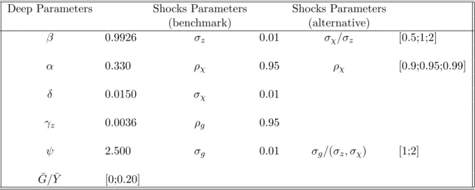
The parameter values are familiar from business cycle literature (see Table 1). We set the capital share to α = 0.33 and the time allocation parameter ψ = 2.5. We choose the discount factor so that the steady state annualized real interest rate is 3%. We set the depreciation rate δ = 0.015. The growth rate of Zt, namely γz, is equal to 0.0036. The share of government consumption in total output at steady state is either 0 or 20%, depending on the version of the model we consider. The parameters of the three forcing variables (Zt, Gt, χt) are borrowed from previous empirical works with US data. The standard–error σz of the technology shock is equal to 1% (see Prescott, 1986, Burnside and Eichenbaum, 1996, Chari, Kehoe and McGrattan, 2007b and Christiano, Eichenbaum and Vigfusson, 2006). Following Christiano and Eichenbaum (1992) and Burnside and Eichenbaum (1996), the autoregressive parameter ρg of government consumption is set to 0.95. The standard error σg is set to 0.01 or 0.02. These two values include previous estimates. We choose alternative values (0.90;0.95;0.99) for the autoregressive parameter ρχ of the preference shock. Previous estimations (see Chari, Kehoe and McGrattan, 2007b and Christiano, Eichenbaum and Vigfusson, 2006) suggest value between 0.95 and 0.99, but we add ρχ = 0.90 for a check of robustness. Finally, the standard error of this shock σχ takes three different values (0.005;0.01;0.02). These values roughly summarize the range of previous estimates (see Erceg, Guerrieri and Gust, 2005, Chari, Kehoe and McGrattan, 2007b, and Christiano, Eichenbaum and Vigfusson, 2006). The alternative calibrations summarize previous estimates which use different datasets and estimation techniques. They allow us to conduct a sensitivity analysis and to evaluate the relative merits of different approaches for various calibrations of the forcing variables.
3
Simulation Results
In our Monte–Carlo study, we generate 1000 data samples from the business cycle model. Every data sample consists of 200 quarterly observations and corresponds to the typical sample size of empirical studies. In order to reduce the effect of initial conditions, the simulated samples include 100 initial points which are subsequently discarded in the estimation. For every data sample, we estimate VAR models with four lags as in Erceg, Guerrieri and Gust (2005), Chari, Kehoe and McGrattan (2007b), and Christiano, Eichenbaum and Vigfusson (2006). We con-sider two versions of the model, depending on the number of shocks included. The two shocks version includes technology shock and preference shocks, whereas the three shocks version adds government consumption. The two shocks version is used so as to evaluate various SVARs with two variables. The three shocks version allows to assess the reliability of three variable SVARs. Moreover, we want to verify if our two step approach properly uncovers the true response of hours when a stationary shock to government consumption affects persistently the consumption
to output ratio.
For each experiment, we investigate the reliability of different SVARs approaches to identify of technology shocks and their aggregate effects: a DSVAR models with labor productivity growth and hours in first difference; a LSVAR model with labor productivity growth and hours in level; a LCYSVAR approach in which the SVAR model includes labor productivity growth and consumption to output ratio in the first step and hours in level are regressed on the estimated technology shock in the second step. The DCYSVAR and CYSVAR–AR(1) approaches are the same in the first step, but they consider hours in first difference and lagged hours in the second step. In the second step of the CYSVAR approach, we consider current and twelve lagged values of the identified (in the first step) technology shocks.11
3.1 Results from the two shock model
In these experiments, government consumption is excluded ( ¯G/ ¯Y = 0). Figures 1 and 2 display the responses of hours for each SVARs in our baseline calibration (ρχ= 0.95 and σz= σχ= 0.01). The solid line represents the response of hours in the model, whereas the dotted line corresponds to the estimated response from SVARs.
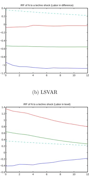
The response of hours obtained from the DSVAR model displays a large downward bias (see figure 1–(a)), and it is persistently negative. This result is similar to Chari, Kehoe and McGrattan (2007b) who show that the difference specification of hours adopted by Gal´ı (1999), Gal´ı and Rabanal (2004) and Francis and Ramey (2005a) can lead to mistaken conclusions about the effect of a technology shock. Note that a DSVAR model is obviously misspecified under the business cycle model considered here, as it implies an over–differentiation of hours. The first difference specification of hours can create distortions and lead to biased estimated responses. However, Chari, Kehoe and McGrattan (2007b) show that SVARs with hours in quasi–difference, consistent with the business cycle model, display similar patterns.
The responses of hours obtained from a LSVAR model displays a large upward bias, as the estimated response on impact is almost twice the true response and is persistently above the true response (see Figure 1–(b)). These results are again in the line with those of Chari, Kehoe and McGrattan (2007b) and to a lesser extent similar with those of Christiano, Eichenbaum and Vigfusson (2006). As reported by Chari, Kehoe and McGrattan (2007b), confidence intervals with the LSVAR model are very large and therefore not informative. The LSVAR cannot discriminate between a model with a positive or a negative effect of the technology shock on impact.12
11We also investigate different lagged values of the technology shock and the main results are left unaffected. 12These very large confidence intervals are not surprising, as long run effects of shocks involve a reliable estimate
of the sum of the VAR parameters. The convergence of the least-squares estimator for the VAR does not imply an accurate approximation of the long run effect (see Sims 1972, Faust and Leeper, 1996 and P¨otscher, 2002).
Consider now the LCYSVAR approach. Figure 2–(a) shows that this approach delivers reliable estimates of the response of hours. The bias is small, especially in comparison with the ones from the DSVAR and LSVAR. Another interesting result is that the three CYSVAR approaches deliver very similar results (see Figures 2–(a), (b) and (c)). Therefore, our two step approach does not suffer from the specification of hours, contrary to the DSVAR and LSVAR. It is worth noting that these small sample experiments support the asymptotic results of Proposition 1. As for the LSVAR, the confidence intervals for LCYSVAR are large. Interestingly, the confidence intervals for DCYSVAR and CYSVAR–AR(1) are narrower on impact than for the LSVAR model. In particular, an one-sided test rejects the hypothesis that the response on impact is negative at the 5% level. These two specifications can then reject an alternative model in which hours decreases on impact after a technology improvement. In contrast, as mentioned by Chari, Kehoe and McGrattan (2007b), the LSVAR is incapable of differentiating between alternative models with starkly different impulse response functions.
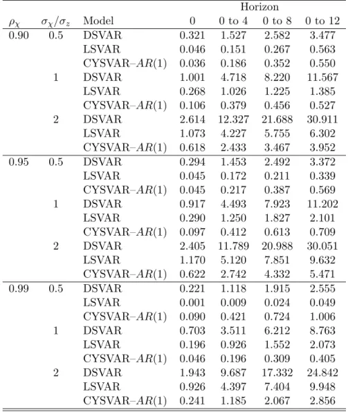
To evaluate the size of the bias, Table 2 reports the cumulative absolute bias between the average response in SVARs and the true response over different horizons.13 In this table, we report only simulation results with the CYSVAR–AR(1) approach since these results are invari-ant to the specification of hours. Our benchmark calibration corresponds to the second panel in Table 2 when ρχ = 0.95 and σχ/σz = 1. We also obtained a large bias with DSVAR and LSVAR models (both on impact and for different horizons). However, The CYSVAR–AR(1) delivers very reliable results compared with DSVAR and LSVAR. We also investigate other calibration of (ρχ, σχ). When the standard error σχ of the non–technology shock is smaller, the accuracy of the LSVAR and DSVAR models increases (see the cases where σχ/σz = 0.5) and the LSVAR model and the CYSVAR–AR(1) approach deliver very similar results. Conversely, when the standard error σχ of the preference increases, the LSVAR and DSVAR models poorly identify the effect of a technology shock on hours (see the cases σχ/σz = 2). In this latter case, the CYSVAR approach tends to over–estimate the true effect of the technology shock, but the cu-mulative absolute mean bias remains small compared to the LSVAR and DSVAR models. Table 2 displays another interesting result: when the persistence of the preference shock increases from 0.9 to 0.99, the bias decreases. For the DSVAR model, this result can be partly explained by a decrease in distortions created by over–differentiation. For the CYSVAR approach, the bias reduction mainly originates from the effect of the preference shock on hours and consumption to output ratio.
The lack of precision of the estimated long run effect is then translated to the impulse response functions.
13This measure is defined as cmd(k) =Pk
i=0|irfi(model) − irfi(svar)| where k denotes the selected horizon, irfi(model) the RBC impulse response and irfi(svar) = (1/N )
PN
j=1irfi(svar)
j the mean of impulse responses
over the N simulation experiments obtained from a SVAR model. In fact, the cmd measures the area of the bias up to the horizon k.
To better understand these last results, we investigate the effect of ρχand σχon the structural autoregressive moving average representation of hours and consumption to output ratio. For our baseline calibration (ρχ= 0.95, σz= σχ= 0.01), we obtain:
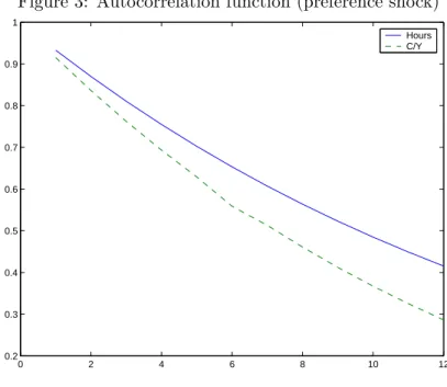
log(Ht) = cst + 0.3536 1 (1 − 0.9622L)σzεz,t− 1.5240 (1 − 0.9759L) (1 − 0.9622L)(1 − 0.95L)σχεχ,t log(Ct) − log(Yt) = cst − 0.4220 1 (1 − 0.9622L)σzεz,t+ 0.8180 (1 − 0.9928L) (1 − 0.9622L)(1 − 0.95L)σχεχ,t, where cst is an appropriate constant. The non–technology component is larger for hours than for consumption to output ratio. In this case, the preference shock accounts for 91% of variance of hours, whereas it represents 63% of the variance of the ratio. Moreover, the persistence of hours generated by the preference shock is more pronounced. This can be seen from the ARMA(2,1) representation of hours and consumption to output ratio. The two series display the same autoregressive parameters, which are associated to the dynamics of capital and the persistence of the preference shock. However, the moving average parameter differs. In the case of hours, the parameter is equal to −0.976, whereas it is −0.993 for the consumption to output ratio. Figure 3 illustrates this property and reports the autocorrelation function of these two variables due to the preference shock. We see that the autocorrelations of the consumption to output ratio are smaller than the ones of hours. The labor wedge has therefore a greater impact in terms of volatility and persistence on hours than on consumption to output ratio. When the standard error of the preference shock is reduced (σχ = 0.005), its contribution to the variance decreases, it becomes 73% for hours and 30% for the consumption to output ratio. In this case, SVARs have less difficulty to disentangle technology shocks from other shocks that have highly persistent, if not permanent effects on labor productivity. This explains why SVARs can properly uncover the true IRFs of hours to a technology shock.
To assess the effect of a highly persistent preference shock, we now set ρχ = 0.99. This situation is of quantitative interest as Christiano, Eichenbaum and Vigfusson (2006) obtain values for this parameter between 0.986 and 0.9994. In this case, the ARMA representation becomes: log(Ht) = cst + 0.3536(1 − 0.9622L)1 σzεz,t− 1.2710(1 − 0.9622L)(1 − 0.99L)(1 − 0.9737L) σχεχ,t log(Ct) − log(Yt) = cst − 0.4220 1 (1 − 0.9622L)σzεz,t+ 0.5167 (1 − 0.9960L) (1 − 0.9622L)(1 − 0.99L)σχεχ,t. The roots of moving average and the autoregressive parameters related to the preference shock in the expression of the consumption to output ratio are very similar,14 so its dynamics can be
14When we set ρ
approximated by a first order autoregressive process:
(log(Ct) − log(Yt)) ' cst + 0.9622(log(Ct−1) − log(Yt−1)) − 0.4220σzεz,t+ 0.5167σχεχ,t. The consumption to output ratio behaves like the deflated capital. Conversely, hours do not share this property and finite autoregressions cannot properly uncover its true dynamics. This is illus-trated in Figure 4 which reports the autocorrelation function of hours, consumption to output ratio and capital deflated by the total factor productivity. As emphasized by Chari, Kehoe and McGrattan (2007b), one of the problem with a SVAR model is that it does not included capital– like variable. In the model, the corresponding relevant state variable is log(Kt/Zt−1). Since Zt is not observable in practice and Kt is measured with errors, we cannot include log(Kt/Zt−1) in SVARs. As can be seen from Figure 4, the autocorrelation functions of (C/Y ) and (K/Z) are very close, but the ones of hours differ sharply.
This latter result suggests that the consumption to output ratio can be a good proxy of the relevant state variable when shocks to labor supply are very persistent or non-stationary. Conversely, hours cannot display this pattern. Highly persistent or non–stationary labor supply shocks is of course debatable but empirical works support this specification in small sample (see Gali, 2005, Christiano, Eichenbaum and Vigfusson, 2006 and Chang, Doh and Schorfheide, 2005). To better understand the results under a close to non–stationary labor supply, we report in appendix C some calculations about the dynamic behavior of the consumption to output ratio and hours for an economy with non stationary labor supply shocks. We notably show that when preference shocks follow a random walk (and thus hours are non–stationary), the consumption to output ratio follows an autoregressive process of order one with an autoregressive parameter exactly equal to the one of the deflated capital. Conversely, the growth rate of hours follows an ARMA process which can be poorly approximated by finite autoregressions. Note that a SVAR model with long–run restrictions that includes labor productivity growth and the consumption to output ratio is valid whatever the process (stationary or non-stationary) of the hours series. The CYSVAR approach allows us to abstract from the very sensitive specification choice of hours in SVARs.
Simulation results for the cumulative absolute bias are completed with a measure of uncer-tainty about the estimated effect of the technology shocks. We thus compute the cumulative Root Mean Square Errors (RMSE) at various horizons.15 The RMSE accounts for both bias and dispersion of the estimated IRFs. The results are reported in Table 3. Simulation experiments
reduced form of the consumption to output ratio is log(Ct) − log(Yt) = 0.3733(1 − 0.9993L)(1 − 0.9622L)−1(1 −
0.999L)−1σ χεχ,t.
15This measure is defined as crmse(k) = Pk
i=0rmsei where k denotes the selected horizon, rmsei =
((1/N )PNj=1(irfi(model) − irfi(svar)j)2)1/2 the RMSE at horizon i, irfi(model) the RBC impulse response
function of hours and irfi(svar)j the SV AR impulse responses function of hours for the jth draw and N is the
for different calibrations show again that the CSVAR approach provides smaller RMSE than the LSVAR and DSVAR models. This result comes essentially from the smaller bias with CSVAR. The large RMSE of DSVAR mainly originates from the large bias. In consequence, DSVAR model displays IRFs that are strongly biased but more precisely estimated. In contrast, LSVAR model displays smaller bias of IRFs but larger dispersion than DSVAR. The CSVAR approach presents the smallest bias on estimated IRFs and the estimated responses are more precisely estimated in comparison with LSVAR. These results from RMSE suggest favoring CYSVAR to LSVAR and DSVAR.
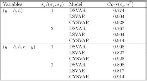
Finally, to judge the identification of the structural shocks, we compute the correlation between the estimated shock and the true shock of the various version of the business cycle model. More precisely, we first compute the correlation between the estimated (from SVARs) and the true technology shocks, namely: Corr(εz, bηT), where ε
z denotes the true technology shock and bηT is the estimated technology shock from SVARs in the first step. We also compute Corr(εχ, bηT), the correlation between the estimated technology shock and non–technology shock εχof the business cycle model. The idea is that if any method is able to consistently estimate the technology shock, we must obtain Corr(εz, bηT) ≈ 1 and Corr(εχ, bηT) ≈ 0. These correlations are reported in Table 4. The CYSVAR approach always delivers the highest Corr(εz, bηT). This correlation is relatively high, as it always exceeds 0.9 and it is not very sensitive to changes in (σz, ρχ, σχ). Conversely, this correlation is lower in the case of the DSVAR model and it decreases dramatically with the volatility of the preference shock. For example, when σχ= 2σz and ρχ = 0.99, the correlation is 0.65 for the DSVAR model, in comparison with 0.91 for the CYSVAR approach. The LSVAR delivers better results that the DSVAR, but it never outperforms the CYSVAR approach.
Let us now examine the correlation between the identified technology shocks of the true preference shocks, namely: Corr(εχ, bηN T). The CYSVAR approach always delivers the lowest correlation (in absolute value). In the case of the DSVAR model, this correlation becomes large (Corr(εχ, bηT) ≈ 0.72) when the variance of the preference shock increases. The large correlation allows to explain why the DSVAR model estimates a negative response of hours to a technology shock. Indeed, the estimated technology shock is contaminated by the preference shock. Hours worked persistently decrease after this shock in the model. It follows that the DSVAR model erroneously concludes that hours drop after a technology shock. A similar result applies in the case of the LSVAR model: the correlation between the estimated technology shock and the true non–technology shock is negative.16. This explains why the LSVAR model over–estimates the effect of a technology shock. In contrast, the CYSVAR approach does not suffer from this
16When σ
contamination.
3.2 Results from the three shock model
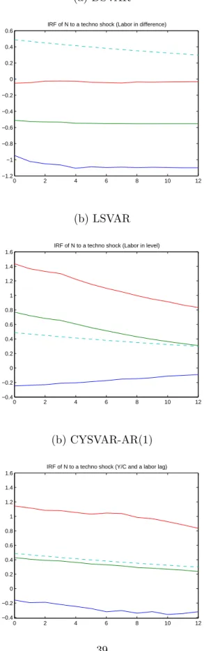
We now add government consumption shocks in the model ( ¯G ¯Y = 0.2 and σg > 0). We first investigate the reliability of SVARs which include two variables (labor productivity and hours for LSVAR and DSVAR models; labor productivity and consumption to output ratio for our two step approach). Figure 5 displays the responses of hours for each SVAR using our baseline calibration (ρχ= ρg = 0.95, σz = σχ = σg = 0.01). As in the case of two shocks, the response of hours obtained from the DSVAR model is downward biased (see Figure 5–(a)) and persistently negative. The response of hours from the LSVAR model is upward biased and the CYSVAR approach delivers again more reliable results. This is confirmed in the first panel of Table 5. For the two values of σg = (0.01; 0.02), the CYSVAR approach outperforms the DSVAR and LSVAR models. Notice that increasing the size of the government consumption shock does not deteriorate the reliability of the two step approach.
From our three shock model, we assess the DSVAR and LSVAR models when they include three variables (labor productivity, hours and consumption to output ratio). Figure 6 reports the responses of hours for the three approaches. Figures 6–(a) and 6–(b) show that SVAR models that include three variables deliver better results. The downward bias of the DSVAR is reduced, as the response on impact becomes positive. Moreover, the upward bias of the LSVAR decreased. However, the DSVAR and LSVAR models do not uncover the true response of hours. These results are in the line with those of Chari, Kehoe and McGrattan (2007b). In our experiments, the CYSVAR approach largely outperforms the DSVAR and LSVAR models (see Table 5). This result is at a first glance surprising, as a three variable SVAR nests a two variable SVAR. Our findings mainly originate in the fact that finite order autoregression cannot properly represent the time series behavior of hours as implied by the model. It follows that hours in SVAR contaminates the estimation of IRFs, even if the consumption to output ratio is included in the VAR model. These results suggest eliminating hours from SVAR models if the objective is to consistently identify technology shocks.
We also report in Table 6 the correlation between the estimated technology shock and the true shock of the business cycle model. We do not report the correlation with individual stationary shocks as we cannot separately identify each of them. The CYSVAR approach delivers again the highest Corr(εz, ηT). This correlation is relatively high, as it always exceeds 0.9 and it is not very sensitive to changes in σg. Conversely, the LSVAR model with three variables provides the lowest correlation, around 0.83. Interestingly, the DSVAR model with three variables performs better than the DSVAR with two variables as the correlation increases from 0.77 to 0.91.
and DSVAR models which use the alternative nonparametric estimator of the long-run covariance matrix proposed by Christiano, Eichenbaum and Vigfusson (2006). In most cases, the CYSVAR approach still outperforms the LSVAR and DSVAR models.17
4
Application of the Two Step Approach
We now apply the two-step methodology with US data. The data used in the SVARs are reported in Figure 7 in appendix. Except for the Federal Fund rate, the data cover the sample period 1948Q1-2003Q4. We first study the dynamic responses of hours work to technology shocks. Second, we investigate the effects of these shocks on the rate of inflation and the nominal interest rate.
4.1 The Dynamic Responses of Hours Worked
We first present results for the IRFs of hours to technology shocks. In the first step, the VAR model includes the growth rate of labor productivity and the log of consumption to output ratio. Labor productivity is measured as the non farm business output divided by non farm business hours worked. Consumption is measured as consumption on nondurables and services and government expenditures. The consumption to output ratio is obtained by dividing the nominal expenditures by nominal GDP. In the second step, the log level ht (see equations (3) and (5)) and the growth rate of hours ∆ht (see equation (4)) are projected on the estimated technology shocks. Hours worked in the non farm business sector are converted to per capita terms using a measure of the civilian population over the age of 16. The period is 1948Q1-2003Q4.
We also compare the estimation results with our two–step approach to those obtained from the estimation of SVAR models. These SVAR models include growth rate of labor productivity, the log of consumption to output ratio and either the log level of hours (LSVAR) or the growth rate of hours (DSVAR). In each of the SVAR models, we identify technology shocks as the only shocks that can affect the long-run level of labor productivity. The lag length p for each VAR model (1) is obtained using the Hannan–Quinn criterion. For each estimated model, we also apply a LM test to check for serial correlation. The number of lags p is 4. For the two-step procedure, we include in the second step the current and twelve past values of the identified technology shocks in the first step, i.e. q = 13 in (3), (4) and (5).
In order to assess the dynamic properties of hours worked and consumption to output ratio (in logs), we first compute their autocorrelation functions (ACFs). Figure 8 reports these ACFs for lags between 1 and 15. As this figure makes clear, the autocorrelation functions of hours worked always exceed those of the consumption to output ratio. Additionally, these ACFs
decay at a slower rate. We also perform Augmented Dickey Fuller (ADF) test of unit root. For each variable, we regress the growth rate on a constant, lagged level and four lags of the first difference. The ADF test statistic is equal to -2.74 for hours and -2.93 for the consumption to output ratio. This hypothesis cannot be rejected at the 5 percent level for hours, whereas it is rejected at the 5 percent level for the consumption to output ratio. These findings suggests that the consumption to output ratio is less persistent than hours.
The estimated IRFs of hours after a technological improvement are reported in Figure 9. The upper left panel shows the well known conflicting results of the effect of a technology shock on hours worked between LSVAR and DSVAR specifications.18 The LSVAR displays a positive hump–shaped response whereas DSVAR implies a decrease in hours. We obtained wide confidence intervals (not reported) in the LSVAR specification, such that the estimated IRFs of hours are not significantly different from zero at any horizon. For the DSVAR specification, the impact response is significant, but as the horizon increase the negative response is not significantly different from zero. In these SVARs, including the consumption to output ratio does not help to reconcile the two specifications.
In contrast, the two-step approach delivers the same picture whether hours are specified in level, first difference or included a lagged term in the regression (see the upper right panel of Figure 9). In the very short run, the IRFs of hours are very similar and when the horizon increases the positive response is a bit more pronounced when hours are taken in level rather than in first difference or with the lagged hours. On impact, hours worked decrease, but after five periods the response becomes persistently positive and hump–shaped.
The bottom panel of Figure 9 reports also the 95 percent asymptotic confidence interval. As previously mentioned, these confidence intervals account for the generated regressor problem and the serial correlation of the errors term in equations (3), (4) and (5). The confidence interval is wide when we consider hours in level (LCYSVAR specification). Consequently, these response cannot be used to discriminate among business cycle theories and for model building. In contrast, when hours are projected in first difference (DCYSVAR specification), the dynamic response are very precisely estimated. On impact, hours significantly decrease. Moreover, the positive hump–shaped response after 8 quarters is precisely estimated. The case of CYSVAR– AR(1) in the second step delivers intermediate results. On impact, the negative response is significant. When the horizon increase, the IRFs are less precisely estimated.
Our findings are in line with those of previous empirical papers which obtain that hours fall significantly on impact (see Gal´ı, 1999, Basu, Fernald and Kimball, 2006, Francis and Ramey, 2005b), but display a hump–shaped positive response during the subsequent periods (see Vig-fusson, 2004).
4.2 The Dynamic Responses of Inflation and Nominal Interest Rate
We now illustrate the potential of our two–step approach by looking at the dynamic responses of the inflation rate and the short–term nominal interest rate after a technology shock. These two variables are known to display high level of serial correlation and some empirical studies have found that they can be characterized by an integrated process of order one.19 Therefore, we use these two variables to illustrate the consequence of the specification choice (level versus first difference) in SVARs.
We first investigate the response of the inflation rate. The measure of inflation is obtained using the growth rate of the GDP deflator. The estimated IRFs of the inflation rate after a technological improvement are reported in Figure 10. As previously, the upper left panel reports the estimated dynamic responses obtained from LSAVR and DSVAR specifications. The DSVAR model includes labor productivity growth, the inflation rate in first difference and the log of consumption to output ratio. The LSVAR model includes the same variables but inflation is considered in level. As this figure shown, the specification of the inflation rate matters. In the DSVAR specification, the rate of inflation responds very little to identified technology shocks. Conversely, the response of inflation in the LSVAR model is persistently negative.
The two-step approach provides similar IRFs according to the specification of the inflation rate in the second step (see the upper right panel of Figure 10). With the LCYSVAR specifi-cation, the dynamic responses are more pronounced but the three specifications of the inflation rate in the second step provide the same shape for the responses. In all cases, the inflation rate decreases on impact and steadily goes back to its long run value. The bottom panel of Figure 10 reports also the 95 percent asymptotic confidence interval. Contrary to hours worked, the confidence interval appears less sensitive to the specification of inflation in the second step. In each regression, the inflation rate significantly decreases in the short run. Note that the effect of a technology improvement has no long–lasting effect on inflation since the response is almost zero after two years. Our finding are again in the line of Basu, Fernald and Kimball (2006). It also complement their results by providing dynamic responses at quarterly frequency.
We now investigate the effect of technology shocks on the short–run nominal interest rate, measured with Federal Fund rate. This rate is available for a shorter sample 1954Q1–2003Q4. Since much of business cycle literature is concerned with post–1959 data, we follow Chris-tiano, Eichenbaum and Vigfusson (2004) and therefore consider a second sample period given 19The empirical results offered in the literature are mixed, depending on the the econometric technique used.
Recent contributions on trend inflation specifies actual inflation as a sum of a random walk and a stationary noise (see Stock and Watson, 2007, Cogley and Sargent, 2007). In Juselius (2006), cointegrated VAR models include the inflation rate and the nominal interest rate in first difference. In the context of permanent technology shocks, Gal´ı (1999) considers a DSVAR model with the inflation rate in first difference and a cointegration between the nominal interest rate and the inflation rate. See also King, Plosser, Stock and Watson (1991) for further evidence of the non–stationarity of these two nominal variables in cointegrated VAR models.
by 1959Q1–2003Q4. The dynamic responses of the nominal interest rate after a technological improvement are reported in Figure 11. In the upper left panel, we report the IRFs obtained from LSVAR and DSVAR specifications. The DSVAR model includes now labor productivity growth, the nominal interest rate in first difference and the log of consumption to output ratio. The LSVAR model includes the same variables but the nominal interest rate is now specified in level. We obtain that the specification of the nominal interest rate modify the dynamic responses of this variable. Notably, the DSVAR specification implies a permanent long run decrease in the nominal interest rate, whereas it steadily goes back to its long run value in the LSVAR specification.
With the two-step approach, the shape of the IRFs is not altered by the specification of the nominal interest rate in the second step (see the upper right panel of Figure 10). However, the dynamic responses with the LCYSVAR specification are more pronounced than the ones of the DCYSVAR and CYSVAR–AR(1) (as for the rate of inflation). In the bottom panel of Figure 11, we report the 95 percent asymptotic confidence interval. For the three specifications in the second step, we obtain a persistent and significant decrease in the Fed Fund rate. These empirical results with quarterly frequency data are again similar to those of Basu, Fernald and Kimball (2006).
5
Conclusion
This paper proposes a simple two step approach to consistently estimate a technology shock and the response of aggregates variables that follows a technology improvement. In a first step, a SVAR model with labor productivity growth and consumption to output ratio allows us to estimate the technology shock. In a second step, the response of hours is obtained by a sim-ple regression of hours on the estimated technology shock. Our approach is motivated by the dynamics of labor productivity and hours which are poorly approximated by finite autoregres-sions. This leads to a large bias in the estimated structural shocks and misleading conclusions about the aggregate effect of a technology shock. When applied to artificial data generated by a standard business cycle model, our approach replicates more closely the model impulse response functions. The estimated technology shock is highly correlated with the true one and the correlation with the non–technology shock is very small. Moreover, the results are invari-ant to the specification of hours in the second step. The two step approach, when applied on actual data, predicts a short–run decrease of hours after a technology improvement, as well as a delayed and hump–shaped positive response. In addition, the rate of inflation and the nominal interest rate displays a significant decrease after a positive technology shock. These findings are in accordance with those of Basu, Fernald and Kimball (2004).
References
Andrews, D.W.K. and J.C. Mohanan (1992) “An Improved Heteroskedasticidy and Autocorre-lation Consistent Covariance Matrix Estimator”, Econometrica, 60, 953–966.
Basu, S., Fernald, J. and M. Kimball (2006) “Are Technology Improvements Contractionary?”, American Economic Review, 96(5), pp. 1418–1448.
Bernanke, B. (1986) ”Alternative Explorations of the Money-Income Correlation,” in: Brunner, Karl and Allan H. Meltzer, eds., Real Business Cycles, Real Exchange Rates, and Actual Policies, Carnegie-Rochester Conference Series on Public Policy, 25, pp. 49–99.
Blanchard, O.J. and D. Quah (1989) “The Dynamic Effects of Aggregate Demand and Supply Disturbances” , American Economic Review, 79(4), pp. 655-673.
Burnside, C. and M. Eichenbaum (1996) “Factor–Hoarding and the Propagation of Business– Cycle Shocks”, American Economic Review, 86(5), pp. 1154–1174.
Chang, Y., Doh, T. and Schorfheide, F. (2005) “Non-stationary Hours in a DSGE Model”, CEPR Discussion Paper 5232.
Chari, V., Kehoe, P. and E. Mc Grattan (2007a) “Business Cycle Accounting”, Econometrica, 75(3), pp. 781–836.
Chari, V., Kehoe, P. and E. Mc Grattan (2007b) “A Critique of Structural VARs Using Real Business Cycle Theory”, Federal Reserve Bank of Minneapolis, Research Department Staff Re-port 364, revised may 2007.
Christiano, L. and M. Eichenbaum (1992) “Current Real–Business–Cycle Theories and Aggre-gate Labor–Market Fluctuations”, American Economic Review, 82(3), pp. 430–450.
Christiano, L., Eichenbaum, M. and C. Evans (1999) “Monetary Policy Shocks: What Have We Learned and to What End?” in Handbook of Macroeconomics, Vol. 1A, ed. J. B. Taylor and M. Woodford, 65ˆu148. Amsterdam:Elsevier.
Christiano, L., Eichenbaum, M. and C. Evans (2005) “Nominal Rigidities and the Dynamic Effects of a Shock to Monetary Policy”, Journal of Political Economy, 113(1), pp. 1-ˆu45. Christiano, L., Eichenbaum, M. and R. Vigfusson (2004) “What Happens after a Technology Shock”, NBER Working Paper Number 9819, revised version 2004.
Christiano, L., Eichenbaum, M. and R. Vigfusson (2006) “Assessing Structural VARs”, NBER Macroeconomics Annual 2006, Volume 21. D. Acemoglu, K. Rogoff and M. Woodford (Eds) Cochrane, J. (1994) “Permanent and Transitory Components of GDP and Stock Returns”, Quarterly Journal of Economics, 109(1), pp. 241–266.
Cogley, T. and T. Sargent (2007) “Inflation-Gap Persistence in the U.S.”, mimeo.
Cooley, T. and S. LeRoy (1985) ”Atheoretical Macroeconometrics: A Critique.” Journal of Monetary Economics, 16, pp. 283–308.
Cooley, T. and M. Dwyer (1998) “Business Cycle Analysis without Much Theory: A Look at Structural VARs”, Journal of Econometrics, 83(1–2), pp. 57–88.
Erceg, C., Guerrieri, L. and C. Gust (2005) “Can Long–Run Restrictions Identify Technology Shocks”, Journal of European Economic Association, 3, pp. 1237–1278.
Faust, J. and E.M. Leeper (1997) “When Do Long-Run Identifying Restrictions Give Reliable Results?”, Journal of Business & Economic Statistics, 15(3), pp. 345–353.
Francis, N. and V. Ramey (2005a) “Is the Technology–Driven Real Business Cycle Hypothesis Dead? Shocks and Aggregate Fluctuations Revisited”, Journal of Monetary Economics, 52, pp. 1379–1399.
Francis, N. and V. Ramey (2005b) “Measures of Per Capita Hours and their Implications for the Technology-Hours Debate”, mimeo UCSD.
Francis, N., Owyang, M. and J. Roush (2005) “A Flexible Finite–Horizon Identification of Technology Shocks”, , Board of Governors of the Federal Reserve System, International Finance Discussion Paper 832, april.
Gal´ı, J. (1999) “Technology, Employment and the Business Cycle: Do Technology Shocks Ex-plain Aggregate Fluctuations?”, American Economic Review, 89(1), pp. 249–271.
Gal´ı, J., and P. Rabanal (2004) “Technology Shocks and Aggregate Fluctuations; How Well does the RBC Model Fit Postwar U.S. Data?”, NBER Macroeconomics Annual, pp. 225–288. Gospodinov, N. (2006) “Inference in Nearly Nonstationary SVAR Models with Long–Run Iden-tifying Restriction”, mimeo Concordia University.
Hall, R. (1997) “Macroeconomic Fluctuations and the Allocation of Time”, Journal of Labor Economics, 15(1), pp. 223–250.
Hansen, L. (1982) “Large Sample Properties of Generalized Method of Moments”, Econometrica, 50, pp. 1029–1054.
Juselius, K. (2006) The Cointegrated VAR model, Advanced Texts in Econometrics, Oxford University Press.
King, R., Plosser, C., Stock, J. and M. Watson (1991) “Stochastic Trends and Economic Fluc-tuations”, American Economic Review, 81(4), pp. 819–840.
Lewis, R. and G.C. Reinsel (1985) “Prediction of Multivariate Time Series by Autoregressive Model Fitting”, Journal of Multivariate Analysis, 15(1), pp. 393–411.
Newey, W.K. (1984) “A Method of Moments Interpretation of Sequential Estimators ”, Eco-nomics Letters, 14, pp. 201–206.
Newey, W.K. and K. West (1994) “Automatic Lag Selection in Covariance Matrix Estimation”, Review of Economic Studies, 61, pp. 631–653.
Pesavento, E. and B. Rossi (2005) “Do Technology Shocks Drive Hours Up or Down”, Macroe-conomic Dynamics, 9(4), pp. 478–488.
Prescott, E. C. (1986) “Theory ahead of business cycle measurement,” Quarterly Review, Federal Reserve Bank of Minneapolis, issue Fall, pages 9-22.
Ravenna, F. (2007) “Vector Autoregressions and Reduced Form Representations of DSGE Mod-els”, Journal of Monetary Economics, 57(7), pp. 2048–2064.
Rotemberg, J. J., and M. Woodford (1997) “An Optimization-Based Econometric Framework for the Evaluation of Monetary Policy”, in NBER Macroeconomics Annual, ed. B. S. Bernanke and J. J. Rotemberg, pp. 297-ˆu346, Cambridge, MA: MIT Press.
Stock, J. and M. Watson (2005) “Why Has U.S. Inflation Become Harder to Forecast?”, Journal of Money, Banking and Credit, 39(1), pp. 3–34.
Vigfusson R. (2004) “The Delayed Response to a Technology Shock. A Flexible Price Expla-nation”, Board of Governors of the Federal Reserve System, International Finance Discussion Paper 810, july.
![Table 3: Simulation Results with two shocks: Cumulative Root Mean Square Errors Horizon ρ χ σ χ /σ z Model 0 [0:4] [0:8] [0:12] 0.90 0.5 DSVAR 0.346 1.683 2.895 3.970 LSVAR 0.224 0.989 1.605 2.163 CYSVAR–AR(1) 0.207 0.962 1.655 2.285 1 DSVAR 1.029 4.899 8.](https://thumb-eu.123doks.com/thumbv2/123doknet/7678532.241674/33.892.197.702.174.769/table-simulation-results-cumulative-square-errors-horizon-cysvar.webp)